On Information Rates of the Fading Wyner Cellular Model via the Thouless Formula for the Strip

Nathan Levy12, Ofer Zeitouni34 and Shlomo Shamai (Shitz)2


1 Département de Mathématiques et Applications, Ecole Normale Supérieure, Paris 75005, France 2 Department of Electrical Engineering, Technion, Haifa 32000, Israel 3 Department of Mathematics, Weizmann Institute of Science, Rehovot 76100, Israel 4 School of Mathematics, University of Minnesota, Minneapolis, MN 55455, USA
Abstract

We apply the theory of random Schrödinger operators to the analysis of multi-users communication channels similar to the Wyner model, that are characterized by short-range intra-cell broadcasting. With $H$ the channel transfer matrix, $HH^{\dagger}$ is a narrow-band matrix and in many aspects is similar to a random Schrödinger operator. We relate the per-cell sum-rate capacity of the channel to the integrated density of states of a random Schrödinger operator; the latter is related to the top Lyapunov exponent of a random sequence of matrices via a version of the Thouless formula. Unlike related results in classical random matrix theory, limiting results do depend on the underlying fading distributions. We also derive several bounds on the limiting per-cell sum-rate capacity, some based on the theory of random Schrödinger operators, and some derived from information theoretical considerations. Finally, we get explicit results in the high-SNR regime for some particular cases.

I Introduction

The growing demand for ubiquitous access to high-data rate services, has produced a huge amount of research analyzing the performance of wireless communications systems. Techniques for providing better service and coverage in cellular mobile communications are currently being investigated by industry and academia. In particular, the use of joint multi-cell processing (MCP), which allows the base-stations (BSts) to jointly process their signals, equivalently creating a distributed antenna array, has been identified as a key tool for enhancing system performance (see [1][2] and references therein for surveys of recent results on multi-cell processing).

Motivated by the fact that mobile users in a cellular system “see” only a small number of BSts, and by the desire to provide analytical results, an attractive analytically tractable model for a multi-cell system was suggested by Wyner in [3] (see also [4] for an earlier relevant work). In this model, the system’s cells are ordered in either an infinite linear array, or in the familiar two-dimensional hexagonal pattern (also infinite). It is assumed that only adjacent-cell interference is present and characterized by a single parameter, a scaling factor $\alpha\in[0,1]$. Considering non-fading channels and a “wideband” (WB) transmission scheme, where all bandwidth is available for coding (as opposed to random spreading), the throughputs obtained with optimum and linear MMSE joint processing of the received signals from all cell-sites are derived in [3]. Since it was first presented, “Wyner-like” models have provided a framework for many works analyzing various transmission schemes in both the up-link and down-link channels (see [1][5] and references therein).

In this paper we consider a generalized “Wyner-like" cellular setup and study its per-cell sum-rate capacity. According to Wyner’s setup, the cells are arranged on a circle (or a line), and the mobile users “see" only a fixed number of BSts which are located close to their cell’s boundaries. All the BSts are assumed to be connected through an ideal back-haul network to a central multi-cell processor (MCP), that can jointly process the up-link received signals of all cell-sites, as well as pre-process the signals to be transmitted by all cell-sites in the down-link channel. The model is characterized by short-range intra-cell broadcasting. Thus, if we denote by $H$ the channel transfer matrix, then $HH^{\dagger}$ is in many aspects similar to a random Schrödinger operator. More specifically, the per-cell sum-rate capacity of the channel is a function of the integrated density of state of $HH^{\dagger}$, which in turn is related to the top Lyapunov exponent of a random sequence of matrices via a version of the Thouless formula. Unlike associated results in classical random matrix theory, limiting results do depend on the underlying fading distributions.

As an application of our result and motivated by the fact that future cellular systems implicitly assume high-SNR configurations mandatory for high data rate services, we get explicit results in the high-SNR regime for some particular cases.

The rest of the paper is organized as follows. In Section II, we present the problem statement. In Section III, we prove the convergence of the per-cell sum-rate capacity when the number of cells and BSts goes to infinity and we express the limit in terms of the Lyapunov exponent of a sequence of random matrices (Theorem 2). In Section IV, we give several reformulations of this result that yields a particularly simple expression in the high-SNR regime. In Section V, we give different bounds on the per-cell sum-rate capacity, some of which are based on the theory of product of random matrices, and some on information theoretical considerations. In Section VI, we specialize the results and make them explicit in some particular cases. Finally in Section VII we discuss some open problems using numerical simulations. The relevant background on the theory of Lyapunov exponents is given in Appendix -A1, and the relevant background on exterior products is given in Appendix -C. Several proofs are postponed to Appendices -A2, -A3 and -B. The per-cell sum-rate capacity of the non-fading channels is derived in Appendix -D.

II Problem statement

In this paper we consider the following setup. $m+d$ cells with $K$ single antenna users per cell are arranged on a line, where the $m$ single antenna BSts are located in the cells. Starting with the WB transmission scheme where all bandwidth is devoted for coding and all $K$ users are transmitting simultaneously each with average power $\rho$, and assuming synchronized communication, a vector baseband representation of the signals received at the system’s BSts is given for an arbitrary time index $i$ by

$$y(i)=H_{m}(i)x(i)+n(i),$$

where $x(i)$ is the $(m+d)K$ complex Gaussian symbols vector, $z(i)$ is the unitary complex Gaussian additive noise vector. Note that the SNR is $\rho$. From now on, we omit the time index $i$. $H_{m}$ is the following $m\times K(m+d)$ channel transfer matrix, which is a $d+1$ block diagonal matrix defined by

$$H_{m}=\begin{pmatrix}\zeta_{1,1}&\zeta_{1,2}&\cdots&\zeta_{1,d+1}&0&\cdots&0\\ 0&\zeta_{2,2}&\cdots&\zeta_{2,d+1}&\zeta_{2,d+2}&&\vdots\\ \vdots&&\ddots&\ddots&&\ddots&0\\ 0&\cdots&0&\zeta_{m,m}&\zeta_{m,m+1}&\cdots&\zeta_{m,d+m}\\ \end{pmatrix},$$

where $\zeta_{i,j}$ are $1\times K$ row vectors. For $s\in{\mathbb{N}}^{*}$, we will denote by $\zeta^{s}$ the vector $(\zeta_{s-d,s},\dots,\zeta_{s,s})$ and we denote by $\pi$ it distribution. We assume in the rest of the paper that for $n\in{\mathbb{N}}^{*}$ and $0\leq i\leq d$ the vectors $(\zeta_{n-i,n})$ are distributed according to $\pi_{i}$. We define $\Omega=(\zeta^{n})_{n\in{\mathbb{N}}^{*}}$ and ${\mathbb{P}}$, the probability distribution on $\Omega$ associated to the above problem. We denote by ${\mathbb{E}}$ the associated expectation. We also use the 2 norm for vectors and matrices. For matrices, it is the Froebenius norm, which is a sub-multiplicative norm.

Throughout this paper, we assume a subset of the following hypotheses.

  1. (H1)

    The vectors $(\zeta^{j})_{j\in{\mathbb{N}}^{*}}$ form a stationary ergodic sequence.

  2. (H2)

    There exists $\varepsilon>0$ such that for $0\leq i\leq d$, ${\mathbb{E}}_{\pi_{i}}\left\lvert\log\left\lvert x\right\rvert\right\rvert^{1+\varepsilon}<\infty$.

  3. (H3)

    If $(x_{0},\dots,x_{d})$ is distributed according to $\pi$, then almost surely, $x_{0}x_{d}^{\dagger}\neq 0$.

For $m\in{\mathbb{N}}^{*}$ and $\lambda>0$, we set $G_{m}=H_{m}H_{m}^{\dagger}+\lambda\operatorname{Id}_{m}$, where $\operatorname{Id}_{m}$ is the $m\times m$ identity matrix. Although $G_{m}$ depends on $\lambda$, we will not write that dependence unless there is an ambiguity. Under the assumption that $H_{m}(i)$ is ergodic with respect to the time index $i$, that the Channel State Information (CSI) is known at the receiver whereas the users know the statistics of the CSI, and that the channel varies fast enough so as to allow each transmitted codeword to experience a large number of fading states, we follow [1] and study the per-cell sum-rate capacity that is given by the following formula ([6])

$$Cap_{m}(\rho)=\frac{1}{m}{\mathbb{E}}\log\det\left(\operatorname{Id}+\rho H_{m}H_{m}^{\dagger}\right)=\log\rho+\frac{1}{m}{\mathbb{E}}\left(\log\det G_{m}(\lambda)\right),$$ (1)

where $\lambda=1/\rho$.

III Main result

We set for $i\in{\mathbb{N}}^{*}$

$\displaystyle C_{i}$ $\displaystyle=\begin{pmatrix}\zeta_{d(i-1)+1,d(i-1)+1}&\zeta_{d(i-1)+1,d(i-1)+2}&\cdots&\zeta_{d(i-1)+1,di}\\ 0&\zeta_{d(i-1)+2,d(i-1)+2}&\cdots&\zeta_{d(i-1)+2,di}\\ \vdots&\ddots&\ddots&\vdots\\ 0&\cdots&0&\zeta_{di,di}\\ \end{pmatrix}$
and
$\displaystyle D_{i}$ $\displaystyle=\begin{pmatrix}{\zeta_{d(i-2)+1,d(i-1)+1}}^{\dagger}&{\zeta_{d(i-2)+2,d(i-1)+1}}^{\dagger}&\cdots&{\zeta_{d(i-1),d(i-1)+1}}^{\dagger}\\ 0&{\zeta_{d(i-2)+2,d(i-1)+2}}^{\dagger}&\cdots&{\zeta_{d(i-1),d(i-1)+2}}^{\dagger}\\ \vdots&\ddots&\ddots&\vdots\\ 0&\cdots&0&{\zeta_{d(i-1),di}}^{\dagger}\\ \end{pmatrix}.$

For all $i\in{\mathbb{N}}^{*}$, $C_{i}$ are $d\times dK$ matrices and $D_{i}$ are $dK\times d$ matrices. We fix $\zeta_{i,j}$ with $i\leq 0$ or $j\leq 0$ so that $C_{1}D_{1}=\operatorname{Id}_{d,d}$.

We thereby get the following block description of $H$

$$H_{dn}=\left(\begin{array}[]{c|c|c|c|c}C_{1}&D_{2}^{\dagger}&0_{d,dK}&\cdots&0_{d,dK}\\ \hline\cr 0_{d,dK}&C_{2}&D_{3}^{\dagger}&\ddots&\vdots\\ \hline\cr\vdots&\ddots&\ddots&\ddots&0_{d,dK}\\ \hline\cr 0_{d,dK}&\cdots&0_{d,dK}&C_{n}&D_{n+1}^{\dagger}\\ \end{array}\right),$$

where $0_{d,dK}$ is the $d\times dK$ zero matrix.

Under the hypothesis (H2), in order to study the limit in $m$ of $Cap_{m}(\rho)$, it is enough to study $Cap_{nd}(\rho)$ (see Remark 32 following the proof of Lemma 25). We get the following block representation of $G_{dn}$:

$$G_{dn}=\left(\begin{array}[]{c|c|c|c}C_{1}C_{1}^{\dagger}+D_{2}^{\dagger}D_{2}+\lambda\operatorname{Id}_{d}&\left(C_{2}D_{2}\right)^{\dagger}&0_{d}&0_{d}\\ \hline\cr C_{2}D_{2}&\ddots&\ddots&0_{d}\\ \hline\cr 0_{d}&\ddots&\ddots&\left(C_{n}D_{n}\right)^{\dagger}\\ \hline\cr 0_{d}&0_{d}&C_{n}D_{n}&C_{n}C_{n}^{\dagger}+D_{n+1}^{\dagger}D_{n+1}+\lambda\operatorname{Id}_{d}\\ \end{array}\right).$$

Note that under (H3), for all $i\in{\mathbb{N}}^{*}$, $C_{i}D_{i}$ is a $d\times d$ invertible matrix.

For $i\in{\mathbb{N}}^{*}$, we denote by $M_{i}$ the following matrix

$$\left(\begin{array}[]{c|c}0_{d}&\operatorname{Id}_{d}\\ \hline\cr-(C_{i+1}D_{i+1})^{-1\dagger}C_{i}D_{i}&-(C_{i+1}D_{i+1})^{-1\dagger}\left(C_{i}C_{i}^{\dagger}+D_{i+1}^{\dagger}D_{i+1}+\lambda\operatorname{Id}_{d}\right)\end{array}\right)$$

and denote $N_{i}=\bigwedge^{d}M_{i}$. Moreover, $\gamma(N)$ denotes the top Lyapunov exponent associated with $\{N_{i}\}$, i.e.

$$\gamma(N)\triangleq\lim_{n\rightarrow\infty}\frac{1}{n}\log\left\lVert N_{n}\cdots N_{1}\right\rVert.$$

Note that by Theorem 20, $\gamma(N)$ is deterministic. See Appendix -A1 for the definitions concerning the Lyapunov exponents and Appendix -C for the relevant background on exterior products. Recall that $(M_{i})_{i\in{\mathbb{N}}^{*}}$ and $(N_{i})_{i\in{\mathbb{N}}^{*}}$ depend on $\lambda$.

Theorem 2

Assume (H1), (H2) and (H3), and set $\lambda=1/\rho$.

  1. 1.

    We have

    $$Cap_{m}(\rho)\xrightarrow[m\rightarrow\infty]{}\log{\rho}+{\mathbb{E}}_{\pi}\log\left\lvert\zeta_{0}\zeta_{d}^{\dagger}\right\rvert+\frac{1}{d}\gamma\left(N\right)\triangleq Cap(\rho),$$

    where the expectation is taken such that $(\zeta_{0},\dots,\zeta_{d})$ is distributed according to $\pi$.

  2. 2.

    As $\rho$ goes to infinity,

    $$Cap(\rho)=\log{\rho}+{\mathbb{E}}_{\pi}\log\left\lvert\zeta_{0}\zeta_{d}^{\dagger}\right\rvert+\frac{1}{d}\gamma\left(N(\lambda=0)\right)+o(1).$$

The theorem is proved in Appendix -A.

As an alternative to deriving exact analytical results we will also be interested in extracting parameters that characterize the channel rate in the high-SNR regime [7]; such parameters are the high-SNR slope (also referred to as the “multiplexing gain")

$$\mathcal{S}_{\infty}\triangleq\lim_{\rho\rightarrow\infty}\frac{Cap(\rho)}{\log(K\rho)},$$

and the high-SNR power offset

$$\mathcal{L}_{\infty}\triangleq\lim_{\rho\rightarrow\infty}\frac{1}{\log 2}\left(\log(K\rho)-\frac{Cap(\rho)}{\mathcal{S}_{\infty}}\right),$$

yielding the following affine capacity approximation

$$Cap(\rho)\approx\frac{\mathcal{S}_{\infty}\log 2}{3|_{\text{dB}}}\left(K\rho|_{\text{dB}}-3|_{\text{dB}}\mathcal{L}_{\infty}\right).$$

A direct consequence of Theorem 2 is the following high-SNR characterization.

Corollary 3

Assume (H1), (H2) and (H3). Then $\mathcal{S}_{\infty}=1$ and

$$\mathcal{L}_{\infty}=\frac{1}{\log 2}\left[\log K-{\mathbb{E}}_{\pi}\log\left\lvert\zeta_{0}\zeta_{d}^{\dagger}\right\rvert-\frac{1}{d}\gamma(N(\lambda=0))\right].$$

IV Reformulations

We now derive alternative formulations for $\gamma(N)$ in Subsection IV-A and for $\gamma(N(\lambda=0))$ (which characterizes the hign-SNR regime), in Subsection IV-B.

IV-A Non-asymptotic results

In order to study $\gamma(N)$, we express it as the Lyapunov exponent of simpler matrices. For $i\geq d+1$, we define the following random matrices.

$$\mathfrak{m}_{i}=\begin{pmatrix}0&1&0&0\\ \vdots&\ddots&\ddots&0\\ 0&\cdots&0&1\\ -\frac{\widetilde{\zeta}_{i,i-d}}{\widetilde{\zeta}_{i,i+d}}&\cdots&\cdots&-\frac{\widetilde{\zeta}_{i,i+d-1}}{\widetilde{\zeta}_{i,i+d}}\end{pmatrix},$$

where $\widetilde{\zeta}_{i,l}$ is the coefficient in position $(i,l)$ in $G_{dn}$, and set

$$\mathfrak{n}_{i}=\bigwedge^{d}\mathfrak{m}_{i}.$$

Note that $(\mathfrak{m}_{i})_{i\geq d+1}$ and $(\mathfrak{n}_{i})_{i\geq d+1}$ depend on $\lambda$. We get the following proposition, whose proof is given in Appendix -B1.

Proposition 4

Assume (H1), (H2) and (H3). Then, $N_{i}=\mathfrak{n}_{id}\cdots\mathfrak{n}_{(i-1)d+1}$. Therefore, for every $\lambda\geq 0$, $\gamma(N)=d\gamma(\mathfrak{n})$, hence,

$$Cap(\rho)=\log\rho+{\mathbb{E}}_{\pi_{0},\pi_{d}}\log\left\lvert\zeta_{0}\zeta_{d}^{\dagger}\right\rvert+\gamma\left(\mathfrak{n}\right).$$

Note that for a given $i\in{\mathbb{N}}$, $N_{i}$ depends on $\zeta^{d(i-1)+1},\dots,\zeta^{(d+1)i}$, that is, the fading coefficients of $2d$ different cells. We now want to reduce the product of the $N_{i}$ to a product of random matrices (that we denote by $\Xi_{i}$) depending on the fading coefficients of only $d$ cells. Then we reduce it further to a product of random matrices (that we denote by $\xi_{i}$) depending on the fading coefficients of only one cell.

By doing so, we achieve two goals: first, we express $\gamma(N)$ as the Lyapunov exponent of simpler matrices. Second, if the fading coefficients are i.i.d for different cells, then the $\Xi_{i}$ and the $\xi_{i}$ are i.i.d. Products of i.i.d random matrices have been studied extensively (see for example [8]), moreover, their study can be reduced to the study of a Markov chain on an appropriate space, which can lead to actual analytic expressions (see [5] for an example of study of such a Markov chain).

For $i\in{\mathbb{N}}^{*}$, we denote by $\Delta_{i}$ the following matrix

$$\left(\begin{array}[]{c|c}-\left(C_{i}C_{i}^{\dagger}+\lambda\operatorname{Id}_{d}\right)(C_{i}D_{i})^{-1\dagger}&-C_{i}D_{i}+\left(C_{i}C_{i}^{\dagger}+\lambda\operatorname{Id}_{d}\right)\left(C_{i}D_{i}\right)^{-1\dagger}D_{i}^{\dagger}D_{i}\\ \hline\cr(C_{i}D_{i})^{-1\dagger}&-\left(C_{i}D_{i}\right)^{-1\dagger}D_{i}^{\dagger}D_{i}\end{array}\right)$$

and define $\Xi_{i}=\bigwedge^{d}\Delta_{i}$.

For $i\geq d+1$, we denote by $\delta_{i}$ the following matrix

(ζid+1,iζid,iζi1,iζid,iIdd10d1,dλ+|ζi,i|2ζid,iζi,i01,d1λζid,iζi,iλζi1,iζi,i0d1,10d1,d10d1,1Idd11ζid,iζi,i01,d1ζid,iζi,iζi1,iζi,i)subscript𝜁𝑖𝑑1𝑖subscript𝜁𝑖𝑑𝑖subscript𝜁𝑖1𝑖subscript𝜁𝑖𝑑𝑖missing-subexpressionmissing-subexpressionmissing-subexpressionsubscriptId𝑑1missing-subexpressionmissing-subexpressionmissing-subexpressionsubscript0𝑑1𝑑missing-subexpressionmissing-subexpressionmissing-subexpressionmissing-subexpressionmissing-subexpressionmissing-subexpressionmissing-subexpressionmissing-subexpressionmissing-subexpression𝜆superscriptsubscript𝜁𝑖𝑖2subscript𝜁𝑖𝑑𝑖superscriptsubscript𝜁𝑖𝑖missing-subexpressionmissing-subexpressionmissing-subexpressionsubscript01𝑑1missing-subexpressionmissing-subexpressionmissing-subexpression𝜆superscriptsubscript𝜁𝑖𝑑𝑖superscriptsubscript𝜁𝑖𝑖𝜆superscriptsubscript𝜁𝑖1𝑖superscriptsubscript𝜁𝑖𝑖missing-subexpressionmissing-subexpressionmissing-subexpressionmissing-subexpressionmissing-subexpressionmissing-subexpressionmissing-subexpressionmissing-subexpressionmissing-subexpressionmissing-subexpressionmissing-subexpressionsubscript0𝑑11missing-subexpressionmissing-subexpressionmissing-subexpressionmissing-subexpressionsubscript0𝑑1𝑑1missing-subexpressionmissing-subexpressionmissing-subexpressionmissing-subexpressionmissing-subexpressionmissing-subexpressionmissing-subexpressionsubscript0𝑑11subscriptId𝑑1missing-subexpressionmissing-subexpressionmissing-subexpressionmissing-subexpressionmissing-subexpressionmissing-subexpressionmissing-subexpressionmissing-subexpressionmissing-subexpressionmissing-subexpressionmissing-subexpression1subscript𝜁𝑖𝑑𝑖superscriptsubscript𝜁𝑖𝑖missing-subexpressionmissing-subexpressionmissing-subexpressionsubscript01𝑑1missing-subexpressionmissing-subexpressionmissing-subexpressionsuperscriptsubscript𝜁𝑖𝑑𝑖superscriptsubscript𝜁𝑖𝑖superscriptsubscript𝜁𝑖1𝑖superscriptsubscript𝜁𝑖𝑖\left(\begin{array}[]{c|ccccccc|c}\begin{array}[]{c}-\frac{\zeta_{i-d+1,i}}{\zeta_{i-d,i}}\\ \vdots\\ -\frac{\zeta_{i-1,i}}{\zeta_{i-d,i}}\end{array}&&&&\operatorname{Id}_{d-1}&&&&0_{d-1,d}\\ \hline\cr-\frac{\lambda+\left\lvert\zeta_{i,i}\right\rvert^{2}}{\zeta_{i-d,i}\zeta_{i,i}^{\dagger}}&&&&0_{1,d-1}&&&&\begin{array}[]{c c c}\lambda\frac{\zeta_{i-d,i}^{\dagger}}{\zeta_{i,i}^{\dagger}}&\cdots&\lambda\frac{\zeta_{i-1,i}^{\dagger}}{\zeta_{i,i}^{\dagger}}\end{array}\\ \hline\cr\begin{array}[]{c}\\ \\ 0_{d-1,1}\\ \\ \\ \end{array}&&&&0_{d-1,d-1}&&&&\begin{array}[]{c|@{\hspace{1cm}}c@{\hspace{1cm}}}\hfil\lx@intercol\vrule\hskip 28.45274pt\\ \hfil\lx@intercol\vrule\hskip 28.45274pt\\ 0_{d-1,1}\hfil\lx@intercol\vrule\hskip 28.45274pt&\operatorname{Id}_{d-1}\hfil\hskip 28.45274pt\\ \hfil\lx@intercol\vrule\hskip 28.45274pt\\ \hfil\lx@intercol\vrule\hskip 28.45274pt\\ \end{array}\\ \hline\cr\frac{1}{\zeta_{i-d,i}\zeta_{i,i}^{\dagger}}&&&&0_{1,d-1}&&&&\begin{array}[]{c c c}-\frac{\zeta_{i-d,i}^{\dagger}}{\zeta_{i,i}^{\dagger}}&\cdots&-\frac{\zeta_{i-1,i}^{\dagger}}{\zeta_{i,i}^{\dagger}}\end{array}\end{array}\right)

and define $\xi_{i}=\bigwedge^{d}\delta_{i}$. Note that $(\Delta_{i})_{i\in{\mathbb{N}}^{*}}$, $(\Xi_{i})_{i\in{\mathbb{N}}^{*}}$, $(\delta_{i})_{i\in{\mathbb{N}}^{*}}$ and $(\xi_{i})_{i\in{\mathbb{N}}^{*}}$ depend on $\lambda$.

Proposition 5

Assume (H1), (H2) and (H3).

  1. 1.

    For every $\lambda\geq 0$, $\gamma(\Xi)=\gamma(N)$, hence,

    $$Cap(\rho)=\log\rho+{\mathbb{E}}_{\pi_{0},\pi_{d}}\log\left\lvert\zeta_{0}\zeta_{d}^{\dagger}\right\rvert+\frac{1}{d}\gamma\left(\Xi\right).$$
  2. 2.

    Assume $K=1$. Then,

    Δi=δidδ(i1)d+1.subscriptΔ𝑖subscript𝛿𝑖𝑑subscript𝛿𝑖1𝑑1\Delta_{i}=\delta_{id}\cdots\delta_{(i-1)d+1}.

    Therefore, for every $\lambda\geq 0$, $\gamma(N)=d\gamma(\xi)$, hence,

    $$Cap(\rho)=\log\rho+{\mathbb{E}}_{\pi_{0},\pi_{d}}\log\left\lvert\zeta_{0}\zeta_{d}^{\dagger}\right\rvert+\gamma\left(\xi\right).$$
Remark 6

Note that for $K=1$, for all $i\in{\mathbb{N}}^{*}$,

$$\left(C_{i}D_{i}\right)^{-1\dagger}=C_{i}^{-1\dagger}D_{i}^{-1\dagger},$$

and therefore,

$$\Delta_{i}=\left(\begin{array}[]{c|c}-C_{i}D_{i}^{-1\dagger}-\lambda(C_{i}D_{i})^{-1\dagger}&\lambda C_{i}^{-1\dagger}D_{i}\\ \hline\cr(C_{i}D_{i})^{-1\dagger}&-C_{i}^{-1\dagger}D_{i}\end{array}\right).$$
Proof of Proposition 5.

Let us start by proving point 1. We define for $i\in{\mathbb{N}}^{*}$,

$$P_{1}(i)=\begin{pmatrix}-C_{i}D_{i}&-C_{i}C_{i}^{\dagger}-\lambda\operatorname{Id}_{d}\\ 0_{d}&\operatorname{Id}_{d}\end{pmatrix}$$

and

$$P_{2}(i)=\begin{pmatrix}0_{d}&\operatorname{Id}_{d}\\ \left(C_{i}D_{i}\right)^{-1\dagger}&-\left(C_{i}D_{i}\right)^{-1\dagger}D_{i}^{\dagger}D_{i}\end{pmatrix},$$

so that for all $i\in{\mathbb{N}}^{*}$, $M_{i}=P_{2}(i+1)P_{1}(i)$. For $i\in{\mathbb{N}}^{*}$, $\Delta_{i}$ is defined so that $\Delta_{i}=P_{1}(i)P_{2}(i)$. Then, for all $n\in{\mathbb{N}}^{*}$,

$\displaystyle M_{n}\dots M_{1}$ $\displaystyle=P_{2}(n+1)P_{1}(n)P_{2}(n)P_{1}(n-1)\cdots P_{2}(2)P_{1}(1)$
$\displaystyle=P_{2}(n+1)\Delta_{n}\cdots\Delta_{2}P_{1}(1).$

and

$\displaystyle\left\lVert N_{n}\dots N_{1}\right\rVert$ $\displaystyle=\left\lVert\bigwedge^{d}P_{2}(n+1)\Xi_{n}\cdots\Xi_{2}\bigwedge^{d}P_{1}(1)\right\rVert$
$\displaystyle\leq\left\lVert\bigwedge^{d}P_{2}(n+1)\right\rVert\left\lVert\Xi_{n}\cdots\Xi_{2}\right\rVert\left\lVert\bigwedge^{d}P_{1}(1)\right\rVert.$

Therefore, $\gamma(N)\leq\gamma(\Xi)$. Since $P_{1}(1)$ and $P_{2}(n+1)$ are invertible, we get the opposite inequality and point 1 is proved.

The proof of point 2 is postponed to Appendix -B2. ∎

IV-B Results in high-SNR regime

Proposition 7

Assume (H1), (H2) and (H3). Assume moreover that $K=1$.

  1. 1.

    For $i\in{\mathbb{N}}^{*}$, we set $\Psi_{i}^{1}=C_{i}D_{i}^{-1\dagger}$ and $\Psi_{i}^{2}=C_{i}^{-1\dagger}D_{i}$. Then

    $$\mathcal{L}_{\infty}=\frac{-1}{\log 2}\left[{\mathbb{E}}_{\pi}\log\left\lvert\zeta_{0}\zeta_{d}^{\dagger}\right\rvert+\frac{1}{d}\max_{0\leq i\leq d}\left(\gamma\left(\bigwedge^{i}\Psi^{1}\right)+\gamma\left(\bigwedge^{d-i}\Psi^{2}\right)\right)\right].$$
  2. 2.

    For $i\geq d+1$, we set

    ψi1=(ζid+1,iζid,iζi,iζid,iIdd101,d1) and ψi2=(ζi1,iζi,iζid,iζi,iIdd101,d1).superscriptsubscript𝜓𝑖1subscript𝜁𝑖𝑑1𝑖subscript𝜁𝑖𝑑𝑖subscript𝜁𝑖𝑖subscript𝜁𝑖𝑑𝑖missing-subexpressionsubscriptId𝑑1missing-subexpressionmissing-subexpressionsubscript01𝑑1 and superscriptsubscript𝜓𝑖2superscriptsubscript𝜁𝑖1𝑖subscript𝜁𝑖𝑖subscript𝜁𝑖𝑑𝑖subscript𝜁𝑖𝑖missing-subexpressionsubscriptId𝑑1missing-subexpressionmissing-subexpressionsubscript01𝑑1\psi_{i}^{1}=\left(\begin{array}[]{@{\hspace{2pt}}c@{\hspace{2pt}}|c}\hskip 2.0pt\lx@intercol\hfil\begin{array}[]{c}-\frac{\zeta_{i-d+1,i}}{\zeta_{i-d,i}}\\ \vdots\\ -\frac{\zeta_{i,i}}{\zeta_{i-d,i}}\end{array}\hfil\hskip 2.0&\begin{array}[]{c}\\ \operatorname{Id}_{d-1}\\ \\ \hline\cr 0_{1,d-1}\end{array}\end{array}\right)\textrm{ and }\psi_{i}^{2}=\left(\begin{array}[]{@{\hspace{2pt}}c@{\hspace{2pt}}|c}\hskip 2.0pt\lx@intercol\hfil\begin{array}[]{c}-\frac{\zeta_{i-1,i}}{\zeta_{i,i}}\\ \vdots\\ -\frac{\zeta_{i-d,i}}{\zeta_{i,i}}\end{array}\hfil\hskip 2.0&\begin{array}[]{c}\\ \operatorname{Id}_{d-1}\\ \\ \hline\cr 0_{1,d-1}\end{array}\end{array}\right)^{\dagger}.

    Then,

    $$\mathcal{L}_{\infty}=\frac{-1}{\log 2}\left[{\mathbb{E}}_{\pi}\log\left\lvert\zeta_{0}\zeta_{d}^{\dagger}\right\rvert+\max_{0\leq i\leq d}\left(\gamma\left(\bigwedge^{i}\psi^{1}\right)+\gamma\left(\bigwedge^{d-i}\psi^{2}\right)\right)\right].$$
Remark 8
  1. 1.

    Recall that for a stationary ergodic sequence of complex random matrices $(X_{i})_{i\in{\mathbb{N}}^{*}}$ of size $d$,

    $$\gamma\left(\bigwedge^{0}X\right)=0\textrm{ and }\gamma\left(\bigwedge^{d}X\right)={\mathbb{E}}\log\left\lvert\det X_{1}\right\rvert.$$
  2. 2.

    Note that if for $0\leq i\leq d$, $\pi_{i}=\pi_{d-i}$ and the vectors $(\zeta_{i})_{i\in{\mathbb{N}}^{*}}$ are i.i.d, then $(\psi_{i}^{1})_{i\geq d+1}$ and $((\psi_{i}^{2})^{\dagger})_{i\geq d+1}$ have the same distribution and $(\psi_{i}^{2})_{i\geq d+1}$ and $((\psi_{i}^{2})^{\dagger})_{i\geq d+1}$ have the same Lyapunov exponents. Therefore, as $\rho$ goes to infinity,

    $$\mathcal{L}_{\infty}=\frac{-1}{\log 2}\left[{\mathbb{E}}_{\pi}\log\left\lvert\zeta_{0}\zeta_{d}^{\dagger}\right\rvert+\gamma\left(\bigwedge^{\left\lceil d/2\right\rceil}\psi^{1}\right)+\gamma\left(\bigwedge^{\left\lfloor d/2\right\rfloor}\psi^{1}\right)\right].$$
Proof of Proposition 7.

Using Corollary 3 and Proposition 5, in order to prove point 1, we only have to prove that

$$\gamma(\Xi(\lambda=0))=\max_{0\leq i\leq d}\left(\gamma\left(\bigwedge^{i}\Psi^{1}\right)+\gamma\left(\bigwedge^{d-i}\Psi^{2}\right)\right).$$ (9)

Recall that $\gamma(\Xi)=\gamma_{1}(\Delta)+\cdots+\gamma_{d}(\Delta)$ and that

$$\Delta_{i}(\lambda=0)=\left(\begin{array}[]{c|c}-\Psi_{i}^{1}&0_{d,d}\\ \hline\cr(C_{i}D_{i})^{-1\dagger}&-\Psi_{i}^{2}\end{array}\right).$$

By Proposition 24, the sequence $\gamma_{1}(\Delta(\lambda=0)),\dots,\gamma_{2d}(\Delta(\lambda=0))$ is equal up to the order to the sequence

$$\gamma_{1}(\Psi^{1}),\dots,\gamma_{d}(\Psi^{1}),\gamma_{1}(\Psi^{2}),\dots,\gamma_{d}(\Psi^{2}).$$

Therefore, (9) is a direct consequence of $\gamma(\Xi(\lambda=0))=\gamma_{1}(\Delta(\lambda=0))+\cdots+\gamma_{d}(\Delta(\lambda=0))$ and $\gamma\left(\bigwedge^{i}\Psi^{1,2}\right)=\gamma_{1}(\Psi^{1,2})+\cdots+\gamma_{i}(\Psi^{1,2})$.

The proof of point 2 goes along the same lines using the fact that

$$\delta_{i}(\lambda=0)=\left(\begin{array}[]{c|c}-\psi_{i}^{1}&0_{d,d}\\ \hline\cr\psi_{i}^{3}&-\widetilde{\psi}_{i}^{2}\end{array}\right),$$

where

$$\widetilde{\psi}_{i}^{2}=\begin{pmatrix}0&0&1\\ 0&\iddots&0\\ 1&0&0\end{pmatrix}\psi_{i}^{2}\begin{pmatrix}0&0&1\\ 0&\iddots&0\\ 1&0&0\end{pmatrix}\textrm{ and }\tilde{\psi}_{i}^{3}=\left(\begin{array}[]{c|c}0_{d-1,1}&0_{d-1,d-1}\\ \hline\cr\frac{1}{\zeta_{i-d,i}\zeta_{i,i}^{\dagger}}&0_{1,d-1}\end{array}\right),$$

therefore, the Lyapunov exponents of $\widetilde{\psi}^{2}$ and $\psi^{2}$ are the same. ∎

V Bounds on the capacity

V-A Bounds on the top Lyapunov exponent

We use the Fröbenius norm on the matrices, it is a sub-multiplicative norm, therefore, we can apply (22) to the different formulations of the capacity to get the following proposition.

Proposition 10

Assume (H1), (H2) and (H3).

  1. 1.

    For $\lambda=1/\rho$ and $p\geq 1$,

    $$Cap(\rho)\leq\log\rho+{\mathbb{E}}_{\pi_{0},\pi_{d}}\log\left\lvert\zeta_{0}\zeta_{d}^{\dagger}\right\rvert+\frac{1}{dp}{\mathbb{E}}\log\left\lVert N_{p}(\lambda)\cdots N_{1}(\lambda)\right\rVert.$$
  2. 2.

    For $\lambda=1/\rho$ and $p\geq 1$,

    $$Cap(\rho)\leq\log\rho+{\mathbb{E}}_{\pi_{0},\pi_{d}}\log\left\lvert\zeta_{0}\zeta_{d}^{\dagger}\right\rvert+\frac{1}{p}{\mathbb{E}}\log\left\lVert\mathfrak{n}_{p}(\lambda)\cdots\mathfrak{n}_{1}(\lambda)\right\rVert.$$
  3. 3.

    For $\lambda=1/\rho$ and $p\geq 1$,

    $$Cap(\rho)\leq\log\rho+{\mathbb{E}}_{\pi_{0},\pi_{d}}\log\left\lvert\zeta_{0}\zeta_{d}^{\dagger}\right\rvert+\frac{1}{dp}{\mathbb{E}}\log\left\lVert\Xi_{p}(\lambda)\cdots\Xi_{1}(\lambda)\right\rVert.$$
  4. 4.

    Assume $K=1$. For $\lambda=1/\rho$ and $p\geq 1$,

    $$Cap(\rho)\leq\log\rho+{\mathbb{E}}_{\pi_{0},\pi_{d}}\log\left\lvert\zeta_{0}\zeta_{d}^{\dagger}\right\rvert+\frac{1}{p}{\mathbb{E}}\log\left\lVert\xi_{p}(\lambda)\cdots\xi_{1}(\lambda)\right\rVert.$$

Moreover, the bounds are tight as $p$ goes to infinity.

The bound of point 2 with $p=1$ can be reformulated as follows.

Corollary 11

For $\lambda=1/\rho$,

$\displaystyle Cap(\rho)\leq\log\rho+$
$\displaystyle\frac{1}{2}{\mathbb{E}}\log\Bigg{[}\binom{2d-2}{d-1}\left(\sum_{l=2}^{2d}\left\lvert\sum_{t=(l-d-1)\vee 0}^{(l-1)\wedge d}\zeta_{d+1,d+t+1}\zeta_{l,d+t+1}^{\dagger}+\lambda{\mathbf{1}}_{(l=d+1)}\right\rvert^{2}\right)+$
$\displaystyle\binom{2d-1}{d}\left(\left\lvert\zeta_{d+1,d+1}\zeta_{1,d+1}^{\dagger}\right\rvert^{2}+\left\lvert\zeta_{d+1,2d+1}\zeta_{2d+1,2d+1}^{\dagger}\right\rvert^{2}\right)\Bigg{]}.$

The proof is postponed to Appendix -B3.

V-B Other bounds

Proposition 12

Assume (H1) and (H2). For $\lambda=1/\rho$,

$\displaystyle\max\left({\mathbb{E}}_{\pi_{0}}\log\left(\lambda+\left\lvert\zeta_{0}\right\rvert^{2}\right),{\mathbb{E}}_{\pi_{d}}\log\left(\lambda+\left\lvert\zeta_{d}\right\rvert^{2}\right)\right)\leq Cap(\rho)-\log\rho\leq$
$\displaystyle{\mathbb{E}}\log\left(\lambda+\left\lvert\zeta_{1,1}\right\rvert^{2}+\cdots+\left\lvert\zeta_{1,d+1}\right\rvert^{2}\right).$
Proof.

The upper bound is a consequence of Hadamard’s inequality for semi-positive definite Hermitian matrices. Indeed,

$$\frac{1}{m}\log\det G_{m}(\lambda)\leq\frac{1}{m}\sum_{i=1}^{m}\log\left(\lambda+\left\lvert\zeta_{i,i}\right\rvert^{2}+\cdots+\left\lvert\zeta_{i,i+d}\right\rvert^{2}\right).$$

Let us show the lower bound of point 12 using the tools of [9].

$\displaystyle Cap_{m}(\rho)$ $\displaystyle=\frac{1}{m}I\left(\boldsymbol{x},\boldsymbol{y}|(\zeta_{i,i})_{1\leq i\leq m},\dots,(\zeta_{i,i+d})_{1\leq i\leq m}\right)$
$\displaystyle=\frac{1}{m}\sum_{j=1}^{m}I\left(x_{j},\boldsymbol{y}|(x_{i})_{1\leq i<j},(\zeta_{i,i})_{1\leq i\leq m},\dots,(\zeta_{i,i+d})_{1\leq i\leq m}\right)$
$\displaystyle\geq\frac{1}{m}\sum_{j=1}^{m}I\left(x_{j},y_{j-d}|(x_{i})_{1\leq i<j},(\zeta_{i,i})_{1\leq i\leq m},\dots,(\zeta_{i,i+d})_{1\leq i\leq m}\right)$
$\displaystyle=\frac{1}{m}\sum_{j=1}^{m}I\left(x_{j},\zeta_{j-d,j}x_{j}+n_{j-d}|\zeta_{j-d,j}\right),$

which is the per-cell sum-rate capacity of a single user fading channel. Therefore, the lower bound is ${\mathbb{E}}_{\pi_{d}}\log\left(1+\rho\left\lvert\zeta_{d}\right\rvert^{2}\right)$.

The role of the distributions $\pi_{0}$ and $\pi_{d}$ can be exchanged by a right-left reflection, namely the transformation $\zeta_{i,j}^{\prime}=\zeta_{m-i+1,m+d-j+1}$. Thus, we get the lower bound. ∎

In the end of this section, we slightly modify the setting, by considering $m$ cells with $K$ single antenna users per cell and $m+d$ single antenna BSts. The communication is characterized by the following $(m+d)\times Km$ channel transfer matrix $H_{m}$, which is a $d+1$ block diagonal matrix defined by,

$$H_{m}=\begin{pmatrix}\zeta_{1,1}&0&\cdots&0\\ \zeta_{2,1}&\zeta_{2,2}&&\vdots\\ \vdots&\vdots&\ddots&0\\ \zeta_{d+1,1}&\zeta_{d+1,2}&&\zeta_{m,m}\\ 0&\zeta_{d+2,2}&&\zeta_{m+1,m}\\ \vdots&&\ddots&\vdots\\ 0&\cdots&0&\zeta_{d+m,m}\end{pmatrix},$$

where $\zeta_{i,j}$ are $1\times K$ row vectors.

We consider the per-cell sum-rate capacity $Cap_{m}(\rho)$ that is given by (1). We denote by $Cap(\rho)$ the limit of $Cap_{m}(\rho)$ as $m$ tends to infinity.

Note that in the limit, this setting is equivalent to the setting we define in Section II. In particular, the normalization by $1/m$ or $1/(m+d)$ is equivalent.

Proposition 13

For all $n\in{\mathbb{N}}^{*}$,

$$\frac{n}{n+d}Cap_{n}\left(\frac{n+d}{n}\rho\right)\leq Cap(\rho)\leq Cap_{n}(\rho).$$

Moreover, the bounds are tight as $n$ goes to infinity.

Note that taking the upper bound for $n=1$, one gets the upper bound of Proposition 12.

Proof.

Number the cells from 1 to $m$ and the antennas from 1 to $m+d$.

Upper bound. Take $1\leq n\leq m$. Consider the following transformation of the communication system: duplicate the antennas number $n+1$ to $n+d$ (each antenna is replaced by two antennas) and denote by $(n+1,a),(n+1,b),\dots,(n+d,a),(n+d,b)$ the new antennas. The cells number $n-d+1$ to $n$ broadcast toward the antennas $(n+1,a),(n+2,a),\dots,(n+d,a)$ and the cells number $n+1$ to $n+d$ broadcast toward the antennas $(n+1,b),(n+2,b),\dots,(n+d,b)$. See Figure 1 for an illustration with $d=2$, $m=8$ and $n=4$. The new system has a higher capacity since a first step of the decoding could be summing up the signals received at antennas $(n+i,a)$ and $(n+i,b)$ ($1\leq i\leq d$) to get the signal received at antenna $n+i$ in the former system. Therefore,

$$mCap_{m}(\rho)\leq nCap_{n}(\rho)+(m-n)Cap_{m-n}(\rho).$$

Take $k\in{\mathbb{N}}^{*}$, by induction,

$$(nk)Cap_{nk}(\rho)\leq(nk)Cap_{n}(\rho).$$

Dividing by $nk$ and taking $k$ to infinity in the LHS gives the upper bound.

Lower bound. Take $k\in{\mathbb{N}}^{*}$ and consider $k(n+d)$ users and their corresponding antennas. For every group of $n+d$ users, silence the $d$ last users and redistribute their power to the $n$ first users so that their SNR becomes $(n+d/n)\rho$ (the average SNR is still $\rho$). See Figure 2 for an illustration. Since asymptotically, the equal power distribution among the users is optimal [10, Appendix C], we get that the new system has a lower capacity. Therefore, for $k$ going to infinity,

$$(nk)Cap_{n}\left(\frac{n+d}{n}\rho\right)\leq k(n+d)Cap_{k(n+d)}(\rho).$$

Dividing by $k(n+d)$ and taking $k$ to infinity in the LHS gives the lower bound. ∎

V-C Numerical comparison of the bounds

We first compare the bound of Corollary 11 and the bounds of Proposition 12. Note that by the ergodic theorem, the upper-bound of Proposition 12 grows like $\log d$, whereas in the bound of Corollary 11, the part $\log\binom{2d-1}{d}\left\lvert\zeta_{d+1,d+1}\zeta_{1,d+1}^{\dagger}\right\rvert^{2}$ alone already grows like $d$. Nevertheless, it is not necessarily true that the upper-bound of Proposition 12 is better that the one of Corollary 11 for all $d$ and all fading distributions.

In Figure 3, we present the bounds of Corollary 11 and Proposition 12 in the special case of Rayleigh fading (real and imaginary parts are independent Gaussian random variables with zero mean and variance $1/\sqrt{2}$). The curves are produced by Monte Carlo simulation with $10^{6}$ samples. We see that in this case, even for $d$ small, the upper-bound of Proposition 12 is better than the one of Corollary 11.

In Figures 4 and 5, we compare the bounds of Proposition 10, point 1 and 3, Proposition 12 and Proposition 13 in the special case of Rayleigh fading (real and imaginary parts are independent Gaussian random variables with zero mean and variance $1/\sqrt{2}$). The curves are produced by Monte Carlo simulations with $10^{5}$ samples.

Note that in the case $d=2$, for $K=1$, the bounds of Proposition 10, point 3 are better than those of point 1, whereas for $K>1$, it is the opposite.

We see that in the case $d=2$, for $K=4$ and $K=10$, the upper-bound of Proposition 12 is very close to the capacity and the upper-bounds of Proposition 10.1 are getting tight very rapidly.

In the case $d=2$, we want to compare the random-fading channel with the non-fading channel. See Appendix -D for the per-cell sum-rate capacity of the non-fading channel. The comparison is done in Figure 5; in the eight cases that we consider, the random-fading channel is better than the non random one.

VI Results for particular cases in the high-SNR regime

VI-A Case $d=1$

As a direct application of Proposition 7 in the case $d=1$ and $K=1$, we get the following result.

Proposition 14

Assume (H1), (H2) and (H3). Then

$$\mathcal{L}_{\infty}=\frac{-1}{\log 2}\left[2\max\left({\mathbb{E}}_{\pi_{0}}\log\left\lvert\zeta_{0}\right\rvert\,;\,{\mathbb{E}}_{\pi_{1}}\log\left\lvert\zeta_{1}\right\rvert\right)\right].$$

Note that a similar result was already proved by other techniques in [5] under much stronger hypothesis, in particular, independence of the fading coefficients was assumed there. In contrary, our result depends only on the marginal distributions of the fading coefficients and is valid for a larger class of joint distributions.

We want to compare the per-cell sum-rate capacity of the random-fading and non-fading channels. For a random variable $\zeta$, by Jensen’s inequality,

$${\mathbb{E}}\log\left\lvert\zeta\right\rvert^{2}\leq\log{\mathbb{E}}\left\lvert\zeta\right\rvert^{2}.$$

Therefore, under the constraints ${\mathbb{E}}_{\pi_{0}}\left\lvert\zeta_{0}\right\rvert^{2}\leq 1$ and ${\mathbb{E}}_{\pi_{1}}\left\lvert\zeta_{1}\right\rvert^{2}\leq 1$, the non-fading channel achieves the best per-cell sum-rate capacity in the high SNR regime.

VI-B Case $d=2$

We now assume that $d=2$ and $K=1$ and that the fading coefficients have the following form; for $i\in{\mathbb{N}}^{*}$,

$$\zeta_{i-2,i}=\alpha a_{i}\ ,\quad\zeta_{i-1,i}=\beta b_{i}\textrm{ and }\zeta_{i,i}=c_{i},$$

where $a_{i}$, $b_{i}$ and $c_{i}$ are random variable distributed according to $\pi_{a}$, $\pi_{b}$ and $\pi_{c}$ respectively and $\alpha$ and $\beta$ are parameters such that $\alpha>0$ and $\beta\geq 0$. Moreover, take the following normalization that can always be achieved by modifying $\alpha$ and $\beta$.

$${\mathbb{E}}_{\pi_{a}}\log\left\lvert a_{1}\right\rvert={\mathbb{E}}_{\pi_{b}}\log\left\lvert b_{1}\right\rvert={\mathbb{E}}_{\pi_{c}}\log\left\lvert c_{1}\right\rvert.$$

We use the notation of Proposition 7.

Proposition 15

Assume that $(a_{i},b_{i},c_{i})_{i\in{\mathbb{N}}^{*}}$ is a stationary ergodic sequence such that for all $i\in{\mathbb{N}}^{*}$, almost surely, $a_{i}$ and $c_{i}$ are non zero and that their exist $\varepsilon>0$ such that ${\mathbb{E}}_{\pi_{a}}\left(\log\left\lvert a_{1}\right\rvert\right)^{1+\varepsilon}$, ${\mathbb{E}}_{\pi_{b}}\left(\log\left\lvert b_{1}\right\rvert\right)^{1+\varepsilon}$ and ${\mathbb{E}}_{\pi_{c}}\left(\log\left\lvert c_{1}\right\rvert\right)^{1+\varepsilon}$ are finite.

Then, there exist a domain ${\cal D}\subset(0,1]\times[0,1]$ such that for all $(x,y)\in{\cal D}$, $(0,x)\times[0,y)\subset{\cal D}$ and for all $(\alpha,\beta)\in{\cal D}$, as $\rho$ goes to infinity,

$$\mathcal{L}_{\infty}=\frac{-2}{\log 2}{\mathbb{E}}_{\pi_{a}}\log\left\lvert a\right\rvert.$$ (16)

The proof is postponed to Appendix -B4.

Remark 17
  1. 1.

    The set ${\cal D}$ is not maximal in the sense that (16) may hold for couples $(\alpha,\beta)\notin{\cal D}$.

  2. 2.

    Note that for $(\alpha,\beta)\in{\cal D}$, in the high-SNR regime, the lower bound of Proposition 12 is tight.

  3. 3.

    The proof will yield an effective construction of ${\cal D}$, which allows us to find many points in ${\cal D}$. Indeed, we construct $(f_{p})_{p\in{\mathbb{N}}^{*}}$ a family of functions on $(0,1]\times[0,1]$ with the following property: if there exists $p\in{\mathbb{N}}^{*}$ such that $f_{p}(\alpha,\beta)\leq 0$, then (16) holds.

  4. 4.

    Note that (16) does not hold when $\alpha>1$, indeed, as it will appear in the course of the proof, as $\rho$ goes to infinity,

    $$Cap(\rho)\geq\log\rho+2{\mathbb{E}}_{\pi_{a}}\log\left\lvert a\right\rvert+\log\alpha.$$

    We conjecture that (16) does not hold when $\beta>1$ either.

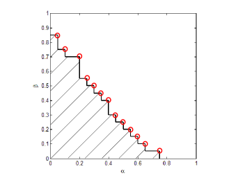
Let us apply Proposition 15 to the case where $(a_{i},b_{i},c_{i})_{i\in{\mathbb{N}}^{*}}$ are independent Rayleigh distributed coefficients. In Figure 6, we plot points for which $f_{20}$ is less or equal to -0.05 (Monte Carlo simulations realized with $10^{5}$ samples). Therefore, (16) holds for $(\alpha,\beta)$ in the stripped region and in particular for $\alpha,\beta\leq 0.4$. Note that in this case, the power offset is

$$\mathcal{L}_{\infty}=\frac{\gamma}{\log 2},$$

where $\gamma$ is the Euler constant.

VI-C Artificial fading

In the frame of non-fading channels, we consider artificial fading, that is, every user uses a pseudo-random fading and multiplies its signal by this artificial fading. The fading coefficients then have the following form, for $i\in{\mathbb{N}}^{*}$ and $0\leq s\leq d$,

$$\zeta_{i,i+s}=\alpha_{s}P_{i+s},$$

where $\alpha_{0},\dots\alpha_{d}$ are non random positive numbers and $P_{i}\,,i\in{\mathbb{N}}^{*}$ are stationary ergodic pseudo-random complex row vectors of size $K$ distributed according to a law denoted by $\pi_{P}$. We moreover assume that for all $i\in{\mathbb{N}}^{*}$, almost surely, the coefficients of $P_{i}$ are non zero and that ${\mathbb{E}}_{\pi_{P}}\left\lVert P_{1}\right\rVert^{2}=1$.

In [11], it is proved that in the case $d=2$, the per-cell sum-rate capacity is smaller with artificial fading. Indeed, had such a procedure helped, then it would be used in non-fading situations to enhance capacity. It is evident then that it is deleterious, as the expression in Proposition 18 exhibits.

We consider the high-SNR regime and derive the explicit influence of the artificial fading.

Proposition 18

Denote by $\mathcal{L}_{\infty}^{0}$ the power off-set without artificial fading (that is, $P_{i}=(1,\dots,1)$ almost surely) and by $\mathcal{L}_{\infty}$ the power off-set with artificial fading. Then,

$$\mathcal{L}_{\infty}=\mathcal{L}_{\infty}^{0}-\frac{1}{\log 2}{\mathbb{E}}_{\pi_{P}}\log\left\lVert P_{1}\right\rVert^{2}.$$
Remark 19

By Jensen’s inequality, we get that $\mathcal{L}_{\infty}\geq\mathcal{L}_{\infty}^{0}$, therefore, in the high-SNR regime, the per-cell sum-rate capacity is smaller with artificial fading.

Proof of Proposition 18.

We set until the end of the proof $\lambda=0$. Using Corollary 3 and Proposition 5,

$$\mathcal{L}_{\infty}=\frac{1}{\log 2}\left[\log K-{\mathbb{E}}_{\pi}\log\left\lvert\alpha_{0}\alpha_{d}^{\dagger}\right\rvert-{\mathbb{E}}_{\pi_{P}}\log\left\lVert P_{1}\right\rVert^{2}-\frac{1}{d}\gamma(\Delta)\right],$$

whereas

$$\mathcal{L}_{\infty}^{0}=\frac{1}{\log 2}\left[\log K-{\mathbb{E}}_{\pi}\log\left\lvert\alpha_{0}\alpha_{d}^{\dagger}\right\rvert-\frac{1}{d}\gamma\left(\widetilde{\Delta}\right)\right],$$

where $\left(\widetilde{\Delta}_{i}\right)_{i\in{\mathbb{N}}^{*}}$ denote the matrices without artificial fading. Therefore, we only have to prove that for $i\in{\mathbb{N}}^{*}$, $\Delta_{i}$ does not depend on $(P_{i})_{i\in{\mathbb{N}}^{*}}$. In the case $K=1$, $\Delta_{i}=\delta_{id}\cdots\delta_{(i-1)d+1}$ and for $i\geq d+1$, $\delta_{i}$ does not depend on $(P_{i})_{i\in{\mathbb{N}}^{*}}$, therefore, $\Delta_{i}$ does not depend on $(P_{i})_{i\in{\mathbb{N}}^{*}}$.

Let us assume $K>1$. Using Proposition 5, we only have to prove that for $i\in{\mathbb{N}}^{*}$, $\Delta_{i}$ does not depend on $(P_{i})_{i\in{\mathbb{N}}^{*}}$.

$\displaystyle C_{i}$ $\displaystyle=\begin{pmatrix}\alpha_{0}P_{d(i-1)+1}&\alpha_{1}P_{d(i-1)+2}&\cdots&\alpha_{d-1}P_{di}\\ 0&\alpha_{0}P_{d(i-1)+2}&\cdots&\alpha_{d-2}P_{di}\\ \vdots&\ddots&\ddots&\vdots\\ 0&\cdots&0&\alpha_{0}P_{di}\\ \end{pmatrix}$
and
$\displaystyle D_{i}$ $\displaystyle=\begin{pmatrix}{\alpha_{d}P_{d(i-1)+1}}^{\dagger}&{\alpha_{d-1}P_{d(i-1)+1}}^{\dagger}&\cdots&{\alpha_{1}P_{d(i-1)+1}}^{\dagger}\\ 0&{\alpha_{d}P_{d(i-1)+2}}^{\dagger}&\cdots&{\alpha_{2}P_{d(i-1)+2}}^{\dagger}\\ \vdots&\ddots&\ddots&\vdots\\ 0&\cdots&0&{\alpha_{d}P_{di}}^{\dagger}\\ \end{pmatrix}.$

Let us define another channel transfer matrix $\widetilde{H}_{m}$ by $\widetilde{K}=1$ and for $i\in{\mathbb{N}}^{*}$ and $0\leq s\leq d$,

$$\widetilde{\zeta}_{i,i+s}=\alpha_{s}\left\lVert P_{i+s}\right\rVert.$$

In the same manner, we define $\widetilde{C}_{i}$, $\widetilde{D}_{i}$ and $\widetilde{\Delta_{i}}$. A straight forward verification shows that for $i\in{\mathbb{N}}^{*}$

$$C_{i}C_{i}^{\dagger}=\widetilde{C}_{i}\widetilde{C}_{i}^{\dagger},\ C_{i}D_{i}=\widetilde{C}_{i}\widetilde{D}_{i}\textrm{ and }D_{i}^{\dagger}D_{i}=\widetilde{D}_{i}^{\dagger}\widetilde{D}_{i}.$$

Moreover, since $\Delta_{i}$ is a function of $C_{i}C_{i}^{\dagger}$, $C_{i}D_{i}$ and $D_{i}^{\dagger}D_{i}$, $\Delta_{i}=\widetilde{\Delta}_{i}$. However, since $\widetilde{K}=1$, we have already proved that $\widetilde{\Delta}_{i}$ does not depend on $(P_{i})_{i\in{\mathbb{N}}^{*}}$, therefore, $\Delta_{i}$ does not depend on $(P_{i})_{i\in{\mathbb{N}}^{*}}$. ∎

VII Numerical simulations

VII-A Influence of the correlation

We assume that the fading coefficients are Rayleigh distributed (real and imaginary parts are independent Gaussian random variables with zero mean and variance $1/\sqrt{2}$) and independent for different users. We are interested in the following question, which of the non-fading channel and the Rayleigh fading channel gives a higher per-cell sum-rate capacity.

In the case $d=2$, $\lambda=0.1,1$ and $K=1,2,4,10$, with all fading coefficients independent, it is shown in Subsection V-C that the Rayleigh fading is beneficial.

In the case $d=1$ if we assume independence between the $\zeta_{i,j}$, it is known that Rayleigh fading is beneficial over non-fading channels in the high-SNR region already for $K=2$ ([5]). If we assume that for $i\in{\mathbb{N}}^{*}$, $\zeta_{i-1,i}=\zeta_{i,i}$, then, the sum-rate per-cell capacity is less than the one of a non-fading channel (see Subsection VI-C and [11]). We investigate the following question: what is the maximal level of correlation between $\zeta_{i-1,i}$ and $\zeta_{i,i}$ that still provides benefit over the non-fading channel. See Appendix -D for the derivation of the capacity of the non-fading channels. We denote by $c$ the correlation between the real (resp. imaginary) part of $\zeta_{i,i}$ and the real (resp. imaginary) part of $\zeta_{i-1,i}$

In Figure 7 we present the bounds of Proposition 10.1 and Proposition 13 in the special case of Rayleigh fading. In Figure 8 we present the bounds of Proposition 10.1 and Proposition 13 in the following special case: $\zeta_{i,i}$ is Rayleigh distributed, $\zeta_{i-1,i}$ is $\alpha\in[0,1]$ times a Rayleigh distributed random variable. In both cases, the curves are produced by Monte Carlo simulation with $10^{5}$ samples.

We see that even with a correlation close to 1, fading still provides an advantage over non-fading channel. Moreover, note that $K$ large, high SNR and $\alpha$ close to 1 are conditions in which the advantage of the fading is larger.

VII-B The asymmetric Wyner model

With the following specification, the model studied is the Rayleigh-fading Wyner model ([3]). We take $d=2$ and the $\zeta_{i,j}$ independent with the following distributions. For $i\in{\mathbb{N}}^{*}$, $\zeta_{i,i+1}$ is Rayleigh distributed (real and imaginary parts are independent Gaussian random variables with zero mean and variance $1/\sqrt{2}$) and $\zeta_{i,i}$ (resp. $\zeta_{i,i+2}$) is $\alpha\in[0,1]$ times a Rayleigh distributed random variable. The asymmetric (Rayleigh-fading) Wyner model is similar to Rayleigh-fading Wyner with a slight modification. For $i\in{\mathbb{N}}^{*}$, $\zeta_{i,i}$ is Rayleigh distributed and $\zeta_{i,i+1}$ (resp. $\zeta_{i,i+2}$) is $\alpha$ times a Rayleigh distributed random variable. Note that in Subsection VI-B we prove that in the asymmetric case, the power offset for $\alpha\leq 0.4$ is $\gamma/\log 2$.

The two models are very similar and yet, in the non-fading case, the per-cell sum-rate capacity is notably different (see Appendix -D for the derivation of the capacity of the non-fading channels). In Figure 9 we present the capacity of the two models without fading and the bounds of Proposition 13 for the two models with Rayleigh fading. We study one case in moderate SNR ($\lambda=1$) and one case in high SNR ($\lambda=10^{-4}$). The curves are produced by Monte Carlo simulation with $10^{5}$ samples.

Note that in the high-SNR region, for the non-fading channel, the per-cell sum-rate capacity is very different for symmetric and the asymmetric models, whereas the per-cell sum-rate capacities for the symmetric and asymmetric Rayleigh-fading models are very close (but not equal as shown in Figure 10 for $\lambda=10^{-4}$ and $\alpha=0.5$).

To understand better the influence of fading on the difference between the two models, we present in Figure 11 the bounds of Proposition 13 for the capacity of the two models (symmetric and asymmetric) with the following fading: the modulus is uniformly distributed between $1-\varepsilon$ and $1+\varepsilon$ and the phase is uniformly distributed between 0 and $2\varepsilon\pi$, where $\varepsilon$ is a parameter between 0 and 1. Note that for $\varepsilon=0$, there is no fading and for $\varepsilon=1$, the fading is uniformly distributed on the disc of center 0 and of radius 2. The curves are produced by Monte Carlo simulation with $10^{5}$ samples. We notice that the difference between the two models decreases between $\varepsilon=0$ and $\varepsilon=0.5$ and that in high-SNR, it increases slightly between $\varepsilon=0.5$ and $\varepsilon=1$.

VIII Concluding Remarks

In this paper, we study the per-cell sum-rate capacity of a channel communication with multiple cell processing. The main tools is a version of the Thouless formula for the strip which we prove in the article. It allows us to prove that the per-cell sum-rate capacity converges as the number of cells and antennas goes to infinity. We give several expressions of the limiting capacity in terms of Lyapunov exponents and several bounds on the per-cell sum-rate capacity.

We apply those results to several examples of communication channels and get insight on the evolution of the capacity as a function of the key parameters of the problem. In particular, in the high-SNR regime, some explicit formulas are derived.

Note that the model here applies verbatim to randomly varying intersymbol interference channels.

Some of the tools of this article can be used to derive CLT-type results on the capacity in order to study the outage-probability. Details will appear elsewhere [12].

Acknowledgments

We thank Oren Somekh for his help with the derivation of the capacity of the non-fading channels.

This research was partially supported by Technion Research Funds, the REMON Consortium, a grant from the Israel Science Foundation and NSF grant DMS-0503775.

-A Random Schrödinger operators techniques

-A1 Lyapunov exponents theory

We use the theory of product of random matrices. For a general introduction to the aspects of the theory we use here, the reader may consult [8], [13], [14], [15], [16] or [17]. See appendix -C for the relevant background on exterior products.

Theorem 20 (Furstenberg H., Kesten H. (1960))

Consider a stationary ergodic sequence of complex random matrices $(X_{i})_{i\in{\mathbb{N}}^{*}}$ of size $p$ and any norm on the matrices. Assume moreover that

$${\mathbb{E}}\log^{+}\left\lVert X_{1}\right\rVert<\infty,$$

then a.s, $n^{-1}\log\left\lVert X_{n}\cdots X_{1}\right\rVert$ converges to a constant:

$$\lim_{n\rightarrow\infty}\frac{1}{n}\log\left\lVert X_{n}\cdots X_{1}\right\rVert\triangleq\gamma(X).$$

We define $p$ constants $\gamma_{1}(X),\dots,\gamma_{p}(X)$ such that for $1\leq i\leq p$,

$$\gamma\left(\bigwedge^{i}X\right)=\gamma_{1}(X)+\cdots+\gamma_{i}(X).$$
Proposition 21
$$\gamma_{1}(X)\geq\cdots\geq\gamma_{p}(X).$$

The constants $\gamma_{1}(X)\geq\cdots\geq\gamma_{p}(X)$ are called the Lyapunov exponents and $\gamma(X)=\gamma_{1}(X)$ is called the top Lyapunov exponent.

We will also use the three following properties:

  1. 1.

    For any sub-multiplicative norm, for $p\in{\mathbb{N}}^{*}$

    $$\gamma(X)\leq\frac{1}{p}{\mathbb{E}}\log\left\lVert X_{p}\cdots X_{1}\right\rVert,$$ (22)

    and the limit of the RHS as $p$ goes to infinity is $\gamma(X)$.

  2. 2.
    $$\frac{1}{p}{\mathbb{E}}\log\left\lvert\det X_{1}\right\rvert\leq\gamma(X).$$ (23)
  3. 3.

    Assume that the matrices $(X_{i})_{i\in{\mathbb{N}}^{*}}$ are i.i.d, then for all $1\leq i\leq p$, $\gamma_{i}(X)=\gamma_{i}(X^{\dagger})$.

Finally, we quote the following proposition [18, Proposition 1].

Proposition 24

Consider a stationary ergodic sequence of complex random matrices $(X_{i})_{i\in{\mathbb{N}}^{*}}$ of size $p$ and any norm on the matrices. Assume moreover that

$${\mathbb{E}}\log^{+}\left\lVert X_{1}\right\rVert<\infty.$$

Finally, assume that there exist three sequences of random matrices $(X_{i}^{1})_{i\in{\mathbb{N}}^{*}}$, $(X_{i}^{2})_{i\in{\mathbb{N}}^{*}}$, $(X_{i}^{3})_{i\in{\mathbb{N}}^{*}}$, of respective sizes $k\times k$, $(p-k)\times k$ and $(p-k)\times(p-k)$, for $1\leq k\leq p-1$, such that almost surely, for all $i$

$$X_{i}=\left(\begin{array}[]{c|c}X_{i}^{1}&0_{k,p-k}\\ \hline\cr X_{i}^{2}&X_{i}^{3}\end{array}\right).$$

Then, $\gamma_{1}(X),\dots,\gamma_{p}(X)$ is equal up to the order to the sequence

$$\gamma_{1}(X^{1}),\dots,\gamma_{k}(X^{1}),\gamma_{1}(X^{3}),\dots,\gamma_{p-k}(X^{3}).$$

-A2 Proof of Theorem 2.1

In order to prove point 1 of Theorem 2, we first prove a slightly more general lemma.

Lemma 25

Assume (H1), (H2) and (H3). For all $\lambda\in{\mathbb{C}}$ such that $\lambda\notin{\mathbb{R}}^{-}$, almost surely,

$$\frac{1}{dn}\log\left\lvert\det G_{dn}\right\rvert\xrightarrow[n\rightarrow\infty]{}\frac{1}{d}{{\mathbb{E}}\log\left\lvert\det(C_{2}D_{2})\right\rvert}+\frac{1}{d}\gamma\left(N\right).$$
Proof.

For $i\in{\mathbb{N}}^{*}$, set $B_{i}=C_{i}C_{i}^{\dagger}+D_{i+1}^{\dagger}D_{i+1}+\lambda\operatorname{Id}_{d}$ and $A_{i}=C_{i}D_{i}$. Note that the eigenvalues of $G_{dn}$ are bounded away from zero. To compute $\log\left\lvert\det G_{dn}\right\rvert$, we write the following decomposition: $G_{dn}U_{dn}=L_{dn}$, where $U_{dn}$ is the upper triangular by block matrix

$$U_{dn}=\left(\begin{array}[]{c|c|c|c}X_{1}&X_{1}&\cdots&X_{1}\\ \hline\cr 0_{d}&X_{2}&\cdots&X_{2}\\ \hline\cr\vdots&\ddots&\ddots&\vdots\\ \hline\cr 0_{d}&\cdots&0_{d}&X_{n}\\ \end{array}\right),$$

the $X_{i}$ are $d\times d$ matrices such that $X_{0}=0_{d}$, $X_{1}=\operatorname{Id}_{d}$, and for $i\geq 1$,

$$A_{i}X_{i-1}+B_{i}X_{i}+A_{i+1}^{\dagger}X_{i+1}=0_{d}.$$ (26)

$L_{dn}$ is the lower triangular by block matrix

$$\left(\begin{array}[]{c|c|c|c}-A_{2}^{\dagger}X_{2}&0_{d}&\cdots&0_{d}\\ \hline\cr A_{2}X_{1}&-A_{3}^{\dagger}X_{3}&\ddots&\vdots\\ \hline\cr 0_{d}&\ddots&\ddots&0_{d}\\ \hline\cr 0_{d}&0_{d}&A_{n}X_{n-1}&-A_{n+1}^{\dagger}X_{n+1}\\ \end{array}\right),$$

That decomposition allows us to write $\log\left\lvert\det G_{dn}\right\rvert$ as a determinant by block,

$\displaystyle\log\left\lvert\det G_{dn}\right\rvert$ $\displaystyle=\sum_{i=1}^{n}\log\left\lvert\det A_{i+1}\right\rvert+\sum_{i=1}^{n}\log\left\lvert\det X_{i+1}\right\rvert-\sum_{i=1}^{n}\log\left\lvert\det X_{i}\right\rvert$
$\displaystyle=\sum_{i=1}^{n}\log\left\lvert\det A_{i+1}\right\rvert+\log\left\lvert\det X_{n+1}\right\rvert.$

Therefore

$$\frac{1}{dn}\log\left\lvert\det G_{dn}\right\rvert=\frac{1}{dn}\sum_{i=1}^{n}\log\left\lvert\det A_{i+1}\right\rvert+\frac{1}{dn}\log\left\lvert\det X_{n+1}\right\rvert.$$ (27)

$\frac{1}{n}\sum_{i=1}^{n}\log\left\lvert\det A_{i+1}\right\rvert$ converges by ergodicity toward ${\mathbb{E}}\log\left\lvert\det A_{2}\right\rvert$. Note that the choice of $A_{n+1}$ is arbitrary, indeed, if we take another value, say $\widetilde{A}_{n+1}$, then $\widetilde{A}^{\dagger}_{n+1}\widetilde{X}_{n+1}=A_{n+1}^{\dagger}X_{n+1}$ and (27) stays unchanged.

We emphasize that the derivation of (27) is inspired by Narula’s thesis ([19]).

The $X_{i}$ are defined by (26). We can reformulate it in the following way. Set $V_{i}=\left(\begin{array}[]{c}X_{i-1}\\ \hline\cr X_{i}\end{array}\right)$, then (26) is equivalent to $V_{i+1}=M_{i}V_{i}$ and moreover,

$$X_{n+1}=\left(\begin{array}[]{c|c}0_{d}&\operatorname{Id}_{d}\end{array}\right)M_{n}\cdots M_{1}\left(\begin{array}[]{c}0_{d}\\ \hline\cr\operatorname{Id}_{d}\end{array}\right).$$

Denote $f=\bigwedge\left(\begin{array}[]{c}0_{d}\\ \hline\cr\operatorname{Id}_{d}\end{array}\right)$. For the relevant background on exterior products, see Appendix -C. We get

$$N_{n}N_{n-1}\dots N_{1}\left(v^{1}_{1}\wedge\dots\wedge v^{d}_{1}\right).$$

However, $v^{1}_{1}\wedge\dots\wedge v^{d}_{1}=f$. Therefore,

$$\begin{split}\det X_{n+1}&=\bigwedge^{d}X_{n+1}=\bigwedge^{d}\left(\left(\begin{array}[]{c|c}0_{d}&\operatorname{Id}_{d}\end{array}\right)M_{n}\cdots M_{1}\left(\begin{array}[]{c}0_{d}\\ \hline\cr\operatorname{Id}_{d}\end{array}\right)\right)\\ &=f^{\dagger}N_{n}N_{n-1}\dots N_{1}f.\end{split}$$ (28)

Taking the canonical basis of $\bigwedge^{d}{\mathbb{C}}^{2d}$, $f$ is the last vector of the basis and $\det X_{n+1}$ grows like the bottom-right coefficient of the product of the $N_{i}$, therefore, its growth rate is bounded above by the Lyapunov exponent of the $N_{i}$.

$$\limsup_{n\rightarrow\infty}\frac{1}{n}{\mathbb{E}}\log\left\lvert\det X_{n+1}\right\rvert\leq\gamma(N).$$ (29)

Using (27), it is enough to prove the opposite inequality to conclude the proof. The end of the proof is inspired by [20].

Lemma 30

If there exist a basis of $\bigwedge^{d}{\mathbb{C}}^{2d}$, say $(g_{i})_{i\in I}$, such that for all $i,j\in I$, almost surely,

$$\liminf_{n\rightarrow\infty}\frac{1}{n}\log\left\lvert g_{j}^{\dagger}N_{n}\cdots N_{1}g_{i}\right\rvert\leq\liminf_{n\rightarrow\infty}\frac{1}{n}\log\left\lvert\det X_{n+1}\right\rvert,$$ (31)

then, almost surely,

$$\gamma(N)\leq\liminf_{n\rightarrow\infty}\frac{1}{n}\log\left\lvert\det X_{n+1}\right\rvert.$$

Let us first prove the lemma.

Proof.

For any finite basis $S_{1}$ and $S_{2}$ in a vector space, we have for all $A$

$$\sup_{\alpha\in S_{1},\beta\in S_{2}}\left\lvert\alpha^{\dagger}A\beta\right\rvert\geq c\left\lVert A\right\rVert$$

for some universal $c$. Thus, (31) shows that, almost surely,

$$\gamma(N)\leq\liminf_{n\rightarrow\infty}\frac{1}{n}\log\left\lvert\det X_{n+1}\right\rvert.$$

To finish the proof of Lemma 25, we denote by $\{e_{1},\dots,e_{2d}\}$ the canonical basis of ${\mathbb{C}}^{2d}$ and we apply the lemma with the following spanning system of $\bigwedge^{d}{\mathbb{C}}^{2d}$

$$S\triangleq\{(e_{1}+\widetilde{e}_{1})\wedge\cdots\wedge(e_{d}+\widetilde{e}_{d})\ ,\ \widetilde{e}_{1},\dots,\widetilde{e}_{d}\in\operatorname{vect}(e_{d+1},\dots,e_{2d})\}.$$

For a choice of $e^{\#}_{1},\dots,e^{\#}_{d}$, such that for $1\leq j\leq d$, $e^{\#}_{j}=\sum_{i=1}^{d}\alpha_{i,j}e_{d+i}$, we define $E^{\#}$ the $d\times d$ matrix of the $\alpha_{i,j}$. We get

$$g_{1}\triangleq(e_{1}+e^{\#}_{1})\wedge\cdots\wedge(e_{d}+e^{\#}_{d})=\bigwedge^{d}\left(\begin{array}[]{c}Id_{d}\\ \hline\cr E^{\#}\end{array}\right).$$

In the same way, for a choice of $e^{b}_{1}\dots,e^{b}_{d}\in\operatorname{vect}(e_{d+1},\dots,e_{2d})$, we define $E^{b}$, a $d\times d$ matrix, such that

$$g_{2}\triangleq(e_{1}+e^{b}_{1})\wedge\cdots\wedge(e_{d}+e^{b}_{d})=\bigwedge^{d}\left(\begin{array}[]{c}Id_{d}\\ \hline\cr E^{b}\end{array}\right).$$

We define two new sequences $(\widetilde{A}_{i})$ and $(\widetilde{B}_{i})$ such that

  • For $2\leq i\leq n-1$, $\widetilde{B}_{i}=B_{i}$,

  • For $1\leq i\leq n$, $\widetilde{A}_{i}=A_{i}$,

  • $\widetilde{B}_{1}=-A_{2}^{\dagger}E^{\#}$,

  • $\widetilde{B}_{n}=A_{n}\left(E^{b}\right)^{\dagger}$,

  • $\widetilde{A}_{n+1}=-A_{n}^{\dagger}$.

We also define $\widetilde{G}_{dn}$, $\widetilde{M}_{i}$, $\widetilde{N}_{i}$ and $\widetilde{X}_{i}$ using $\left(\widetilde{A}_{i}\right)_{i\in{\mathbb{N}}^{*}}$ and $\left(\widetilde{B}_{i}\right)_{i\in{\mathbb{N}}^{*}}$. Then,

$\displaystyle f^{\dagger}\widetilde{N}_{n}\widetilde{N}_{n-1}\dots\widetilde{N}_{1}f$ $\displaystyle=f^{\dagger}\bigwedge^{d}\left(\begin{array}[]{c|c}0_{d}&\operatorname{Id}_{d}\\ \hline\cr\operatorname{Id}_{d}&\left(E^{b}\right)^{\dagger}\end{array}\right)\widetilde{N}_{n-1}\dots\widetilde{N}_{2}\bigwedge^{d}\left(\begin{array}[]{c|c}0_{d}&\operatorname{Id}_{d}\\ \hline\cr-T_{1}T_{2}^{-1\dagger}&E^{\#}\end{array}\right)f$
$\displaystyle=g_{2}^{\dagger}\widetilde{N}_{n-1}\dots\widetilde{N}_{2}g_{1}.$

Therefore, to prove the condition (31), it is enough to prove that, almost surely,

$$\limsup_{n\rightarrow\infty}\left(\frac{1}{n}\log\left\lvert\det\widetilde{G}_{dn}\right\rvert-\frac{1}{n}\log\left\lvert\det{G_{dn}}\right\rvert\right)\leq 0.$$

We now use perturbation theory techniques. Indeed, we denote by $\rho$ the spectral radius of a matrix, i.e. its largest eigenvalue in absolute value. Recall that for a matrix $S$, $\rho(S)\leq\sqrt{\rho(SS^{\dagger})}$ and that $\sqrt{\rho(SS^{\dagger})}$ is a sub-multiplicative norm. As a consequence, for positive Hermitian matrices, the spectral radius is sub-multiplicative. Moreover, we denote by $\left\lVert\cdot\right\rVert_{F}$ the Fröbenius norm. Recall that $\sqrt{\rho(SS^{\dagger})}\leq\left\lVert S\right\rVert_{F}$. We will also use the fact that the eigenvalues of $G_{dn}$ are bounded away from 0 by $\mu=\lambda$ if $\lambda>0$ or $\mu=\left\lvert\Im\lambda\right\rvert$ if $\lambda\notin{\mathbb{R}}$. Moreover, we define $U_{dn}=\widetilde{G}_{dn}-G_{dn}$, which has rank less than or equal to $2d$.

$\displaystyle\frac{1}{n}\log\left\lvert\det\widetilde{G}_{dn}\right\rvert-\frac{1}{n}\log\left\lvert\det{G_{dn}}\right\rvert$ $\displaystyle=\frac{1}{n}\log\left\lvert\det(G_{dn}+U_{dn})\right\rvert-\frac{1}{n}\log\left\lvert\det{G_{dn}}\right\rvert$
$\displaystyle=\frac{1}{n}\log\left\lvert\det(\operatorname{Id}_{dn}+G_{dn}^{-1}U_{dn})\right\rvert.$

$G_{dn}^{-1}U_{dn}$ has rank at most 2d, therefore,

$\displaystyle\frac{1}{n}\log\left\lvert\det\widetilde{G}_{dn}\right\rvert-\frac{1}{n}\log\left\lvert\det{G_{dn}}\right\rvert$ $\displaystyle\leq\frac{2d}{n}\log\left\lvert 1+\rho(G_{dn}^{-1}U_{dn})\right\rvert$
$\displaystyle\leq\frac{2d}{n}\log\left\lvert 1+\sqrt{\rho(G_{dn}^{-1}U_{dn}U_{dn}^{\dagger}G_{dn}^{-1\dagger})}\right\rvert$
$\displaystyle\leq\frac{2d}{n}\log\left\lvert 1+\sqrt{\rho(G_{dn}^{-1\dagger}G_{dn}^{-1})}\sqrt{\rho(U_{dn}U_{dn}^{\dagger})}\right\rvert$
$\displaystyle\leq\frac{2d}{n}\log\left\lvert 1+\frac{1}{\mu}\sqrt{\rho(U_{dn}U_{dn}^{\dagger})}\right\rvert$
$\displaystyle\leq\frac{2d}{n}\log\left\lvert 1+\frac{1}{\mu}\left\lVert U_{dn}\right\rVert_{F}\right\rvert.$

Moreover,

$$\left\lVert U_{dn}\right\rVert_{F}^{2}=\left\lVert S_{1}+\lambda\operatorname{Id}_{d}+T_{2}^{\dagger}E^{\#}\right\rVert_{F}^{2}+\left\lVert S_{n}+\lambda\operatorname{Id}_{d}+T_{n}^{\dagger}E^{b}\right\rVert_{F}^{2},$$

hence, with the integrability condition, $\sup_{n}{\mathbb{E}}\log\left\lvert 1+\frac{1}{\mu}\left\lVert U_{dn}\right\rVert_{F}\right\rvert^{1+\varepsilon}<\infty$. By Tchebicheff inequality, for a given $\eta>0$,

$${\mathbb{P}}\left(\frac{1}{n}\log\left\lvert 1+\frac{1}{\mu}\left\lVert U_{dn}\right\rVert_{F}\right\rvert>\eta\right)\leq\frac{\sup_{n}{\mathbb{E}}\log\left\lvert 1+\frac{1}{\mu}\left\lVert U_{dn}\right\rVert_{F}\right\rvert^{1+\varepsilon}}{(\eta n)^{1+\varepsilon}}.$$

The RHS is a summable series, therefore, by Borel-Cantelli Lemma, almost surely,

$$\limsup_{n\rightarrow\infty}\left(\frac{1}{n}\log\left\lvert\det\widetilde{G}_{dn}\right\rvert-\frac{1}{n}\log\left\lvert\det{G_{dn}}\right\rvert\right)\leq 0.$$

This finishes the proof of Lemma 25. ∎

Remark 32

By the same kind of perturbation theory techniques, we can show that in order to study the limit in $m$ of $Cap_{m}(\rho)$, it is enough to study the sequence every $d$ steps.

For a hermitian matrix $h$ whose ordered eigenvalues are $\alpha_{1},\dots,\alpha_{n}$, we denote by the spectral distribution of $h$, the measure

$$\frac{1}{n}\sum_{i=1}^{n}\delta_{\alpha_{i}},$$

where $\delta_{x}$ is a Dirac measure at $x$.

The following technical lemma will be used several times to prove domination properties.

Lemma 33

Denote by $\mu_{n}$ the spectral distribution of $H_{dn}H_{dn}^{\dagger}$. Consider the following diagonal by blocks matrix:

$$F_{dn}\triangleq\left(\begin{array}[]{c|c|c|c}2B_{1}&0_{d}&\cdots&0_{d}\\ \hline\cr 0_{d}&2B_{2}&\ddots&\vdots\\ \hline\cr\vdots&\ddots&\ddots&0_{d}\\ \hline\cr 0_{d}&\cdots&0_{d}&2B_{n}\\ \end{array}\right),$$

and denote by $\tilde{\mu}_{n}$ its spectral distribution. Then, for any non-decreasing function $f$,

$$\int fd\mu_{n}\leq\int fd\tilde{\mu}_{n}.$$
Proof.

Denote

$$\tilde{H}_{dn}=\left(\begin{array}[]{c|c|c|c|c}C_{1}&-D_{2}^{\dagger}&0_{d,dK}&\cdots&0_{d,dK}\\ \hline\cr 0_{d,dK}&C_{2}&-D_{3}^{\dagger}&\ddots&\vdots\\ \hline\cr\vdots&\ddots&\ddots&\ddots&0_{d,dK}\\ \hline\cr 0_{d,dK}&\cdots&0_{d,dK}&C_{n}&-D_{n+1}^{\dagger}\\ \end{array}\right),$$

then $F_{dn}=H_{dn}H_{dn}^{\dagger}+\tilde{H}_{dn}\tilde{H}_{dn}^{\dagger}$. Since $\tilde{H}_{dn}\tilde{H}_{dn}^{\dagger}$ is a non-negative Hermitian matrix, by Weyl’s inequalities, for all $1\leq i\leq dn$, the $i$-th eigenvalue of $H_{dn}H_{dn}^{\dagger}$ is less or equal than the $i$-th eigenvalue of $F_{dn}$. ∎

First note that $(1/d){{\mathbb{E}}\log\left\lvert\det(C_{2}D_{2})\right\rvert}={\mathbb{E}}_{\pi}\log\left\lvert\zeta_{0}\zeta_{d}^{\dagger}\right\rvert$. From Lemma 33, we deduce that for $\lambda>0$,

$$\frac{1}{dn}\log\left\lvert\det G_{dn}\right\rvert\leq\log 2+\frac{1}{n}\sum_{i=1}^{n}\log\left\lvert\det B_{i}\right\rvert.$$

Therefore by (H2) and Hadamard’s inequality, $(1/dn)\log\left\lvert\det G_{dn}\right\rvert$ is a uniformly integrable sequence and the almost sure convergence of Lemma 25 implies point 1 of Theorem 2.

-A3 Proof of Theorem 2.2

We begin by a few notations. For $\lambda\notin{\mathbb{R}}$, set

$$f(\lambda)=\lim_{n\rightarrow\infty}\frac{1}{dn}\log\left\lvert\det\left(H_{dn}H_{dn}^{\dagger}+\lambda\operatorname{Id}_{dn}\right)\right\rvert,$$

which exists by Lemma 25. The existence of the weak limit of $\mu_{n}$ and the fact that it is non random is a classical fact of the random Schrödinger operators theory, see for example [16, Theorem 4.4]. For $\lambda\in{\mathbb{C}}$, we set (if it exists)

$$g(\lambda)=\int\log\left\lvert x+\lambda\right\rvert d\mu(x).$$

We emphasize that since $\log$ is not a bounded function, we cannot directly deduce from Lemma 25 and the weak convergence of the $\mu_{n}$ to $\mu$ that for $\lambda\notin{\mathbb{R}}$, $f(\lambda)=g(\lambda)$.

Finally, for $\lambda\in{\mathbb{C}}$, define

$$h(\lambda)={\mathbb{E}}_{\pi}\log\left\lvert\zeta_{0}\zeta_{d}^{\dagger}\right\rvert+\frac{1}{d}\gamma\left(N\right).$$

The following lemma is a generalization of the Thouless formula for the strip proved in [20].

Lemma 34

Assume (H1), (H2) and (H3). For all $\lambda\in{\mathbb{C}}$, $g(\lambda)=h(\lambda)$.

The proof of this result is done in the frame of channel transfer matrices but one does not need to assume that the $A_{i}$ and the $B_{i}$ are upper triangular by blocks, one just need instead of (H3) the hypothesis that almost surely, $A_{i}B_{i}$ is invertible.

Proof.

The proof goes along the following lines, we first prove that for $\lambda\notin{\mathbb{R}}$, $g(\lambda)$ exists and equals to $h(\lambda)$, then, following [21] we argue that $g$ and $h$ are two subharmonic functions equal everywhere except a set of 0 measure, therefore they are equal everywhere.

Step 1: Let us first prove that for $\lambda\notin{\mathbb{R}}$, $g(\lambda)$ is well defined. $\log\left\lvert x+\lambda\right\rvert$ is bounded away from $-\infty$, therefore, $g(\lambda)$ exists although it may be $\infty$. For $R\geq 0$, let us denote by $\log_{R}$ the function $t\rightarrow\log(t)\wedge R$. By monotone convergence, it is enough to prove that $\int\log_{R}\left\lvert x+\lambda\right\rvert d\mu(x)$ is bounded uniformly in $R$. Since $x\rightarrow\log_{R}\left\lvert x+\lambda\right\rvert$ is a bounded continuous function,

$$\int\log_{R}\left\lvert x+\lambda\right\rvert d\mu(x)=\lim_{n\rightarrow\infty}\int\log_{R}\left\lvert x+\lambda\right\rvert d\mu_{n}(x).$$

By Lemma 33, and using that $\int\log_{R}\left\lvert x+\lambda\right\rvert d\mu_{n}(x)\leq\int\log\left\lvert x+\lambda\right\rvert d\mu_{n}(x)$,

$$\lim_{n\rightarrow\infty}\int\log_{R}\left\lvert x+\lambda\right\rvert d\mu_{n}(x)\leq\lim_{n\rightarrow\infty}\int\log\left\lvert x+\lambda\right\rvert d\tilde{\mu}_{n}(x)={\mathbb{E}}\log\left\lvert\det B_{1}\right\rvert<\infty,$$

where the last inequality comes from (H2) and Hadamard’s inequality. Finally, we get that for $\lambda\notin{\mathbb{R}}$,

$$g(\lambda)\leq{\mathbb{E}}\log\left\lvert\det B_{1}\right\rvert<\infty.$$

Step 2: Let us prove that for $\lambda\notin{\mathbb{R}}$, $f(\lambda)=g(\lambda)$. Applying Lemma 33 one shows that for $\lambda\notin{\mathbb{C}}$, the sequence $\left(\int\log\left\lvert x+\lambda\right\rvert d\mu_{n}(x)\right)_{n\in{\mathbb{N}}^{*}}$ is uniformly integrable and therefore,

$$f(\lambda)=\lim_{n\rightarrow\infty}{\mathbb{E}}\int\log\left\lvert x+\lambda\right\rvert d\mu_{n}(x).$$

By Lemma 33, for $R\geq 0$,

$\displaystyle{\mathbb{E}}\int_{x\geq R}\log\left\lvert x+\lambda\right\rvert d\mu_{n}(x)$ $\displaystyle\leq{\mathbb{E}}\int_{x\geq R}\log\left\lvert x+\lambda\right\rvert d\tilde{\mu}_{n}(x)$
$\displaystyle={\mathbb{E}}\int_{x\geq R}\log\left\lvert x+\lambda\right\rvert d\tilde{\mu}_{1}(x).$

Therefore, for $n\in{\mathbb{N}}^{*}$ and $R\geq 0$,

$\displaystyle\left\lvert{\mathbb{E}}\int\log\left\lvert x+\lambda\right\rvert d\mu_{n}(x)-g(\lambda)\right\rvert\leq\left\lvert{\mathbb{E}}\int_{x\geq R}\log\left\lvert x+\lambda\right\rvert d\tilde{\mu}_{1}(x)\right\rvert$
$\displaystyle\qquad\qquad\qquad\qquad+\left\lvert{\mathbb{E}}\int\log_{R}\left\lvert x+\lambda\right\rvert d\mu_{n}(x)-{\mathbb{E}}\int\log_{R}\left\lvert x+\lambda\right\rvert d\mu(x)\right\rvert$
$\displaystyle\qquad\qquad\qquad\qquad+\left\lvert{\mathbb{E}}\int_{x\geq R}\log\left\lvert x+\lambda\right\rvert d\mu(x)\right\rvert.$

We first fix $R\geq 0$ such that the first and the third terms are arbitrary small and then, by weak convergence, the second term goes to 0 as $n$ goes to infinity. Therefore, for $\lambda\notin{\mathbb{R}}$, $f(\lambda)=g(\lambda)$ and by Lemma 25, $g(\lambda)=h(\lambda)$.

Step 3: Let us prove that $g$ and $h$ are subharmonic on ${\mathbb{C}}$. See [21] for the relevant definitions. Since for $i\in{\mathbb{N}}^{*}$, $N_{i}(\lambda)$ is an entire function of $\lambda$, $h$ is subharmonic ([21]).

Let us prove that $g$ is subharmonic. For $R\geq 0$, set

$$g_{R}(\lambda)\triangleq\int\left(\log\left\lvert x+\lambda\right\rvert\vee-R\right)d\mu(x).$$

By Lemma 33, $g_{R}$ a continuous function. As $R$ goes to infinity, $g_{R}$ is a decreasing sequence of functions converging point wise to $g$, therefore, $g$ is subharmonic.

The functions $g$ and $h$ are subharmonic on ${\mathbb{C}}$ and equal on ${\mathbb{C}}-{\mathbb{R}}$, therefore, $g$ and $h$ are equal on ${\mathbb{C}}$. ∎

To finish the proof of point 2 of Theorem 2, let us prove that $h(\lambda)$ converges to $h(0)$ when $\lambda$ goes to 0 in ${\mathbb{R}}^{+}$. Note that ${\mathbb{E}}\log\left\lvert\det M_{1}\right\rvert=0$, therefore, ${\mathbb{E}}\log\left\lvert\det N_{1}\right\rvert=0$. By (23), $h(0)\geq{\mathbb{E}}_{\pi}\log\left\lvert\zeta_{0}\zeta_{d}^{\dagger}\right\rvert$, therefore, using Lemma 33 and the fact that for $\lambda,x\in{\mathbb{R}}^{+}$, $\log\left\lvert x+\lambda\right\rvert\geq\log\left\lvert x\right\rvert$, we get the desired result.

-B Other proofs

-B1 Proof of Proposition 4

We use the notation of Subsection -A2. We define $x^{i}_{j}$ for $i\in{\mathbb{N}}$ and $1\leq j\leq d$ such that the the element at the position $(s,t)$ of $X_{i}$ is $x^{(i-1)d+s}_{t}$. Recall that $G_{dn}U_{dn}=L_{dn}$. Therefore, for a given $j$ such that $1\leq j\leq d$, we get the following characterization of the sequence $(x^{i}_{j})_{i}$. $x^{i}_{j}=0$ for $-d+1\leq i\leq 0$, $x^{i}_{j}=\delta_{i,j}$ for $1\leq i\leq d$ and for $i\geq d+1$,

$$\sum_{l=i-d}^{i+d}\widetilde{\zeta}_{i,l}x_{j}^{l}=0.$$ (35)

Therefore,

$$\begin{pmatrix}x^{i-d+1}_{j}\\ \vdots\\ x^{i+d}_{j}\end{pmatrix}=\mathfrak{m}_{i}\begin{pmatrix}x^{i-d}_{j}\\ \vdots\\ x^{i+d-1}_{j}\end{pmatrix}.$$

Moreover,

$\displaystyle V_{i+1}$ $\displaystyle=\begin{pmatrix}x_{1}^{(i-1)d+1}&\cdots&x_{d}^{(i-1)d+1}\\ \vdots&&\vdots\\ x_{1}^{(i+1)d}&\cdots&x_{d}^{(i+1)d}\\ \end{pmatrix}$
$\displaystyle=\mathfrak{m}_{id}\cdots\mathfrak{m}_{(i-1)d+1}\begin{pmatrix}x_{1}^{(i-2)d+1}&\cdots&x_{d}^{(i-2)d+1}\\ \vdots&&\vdots\\ x_{1}^{id}&\cdots&x_{d}^{id}\\ \end{pmatrix}$
$\displaystyle=\mathfrak{m}_{id}\cdots\mathfrak{m}_{(i-1)d+1}V_{i}.$

Therefore, together with 26, it proves Proposition 4.

-B2 Proof of Proposition 5.2

In order to prove point 2 of Proposition 5, we first prove the following lemma:

Lemma 36

For all $i\geq d+1$, there exist matrices $p^{s}_{1}(i)$, $p^{s}_{2}(i)$ for $1\leq s\leq d$ and $\delta^{s}(i)$ for $1\leq s\leq d+1$ such that $\delta^{1}(i)=\mu(i)$, $\delta^{s}(i)=\underline{\delta}^{s}(\zeta^{i},\dots,\zeta^{i+d-s+1})$, $p^{s}_{1}(i)=\underline{p}^{s}_{1}(\zeta^{i},\dots,\zeta^{i+d-s})$ and $p^{s}_{2}(i)=\underline{p}^{s}_{2}(\zeta^{i+d-s})$, where $\underline{\delta}^{s}$, $\underline{p}^{s}_{1}$ and $\underline{p}^{s}_{2}$ are deterministic functions. We have moreover the two relationships

$$\delta^{s}(i)=p^{s}_{2}(i+1)p^{s}_{1}(i).$$ (37)
$$\delta^{s+1}(i)=p^{s}_{1}(i)p^{s}_{2}(i).$$ (38)

Finally, for $i\geq d+1$, $\delta_{i}=\delta^{d+1}(i)$

Proof.

For $i\geq d+1$ and $1\leq s\leq d$, define

  • for $s\leq l\leq 2d$,

    $$a^{i,s}_{l}=-\lambda{\mathbf{1}}_{(l=d+s)}-\sum_{t=(l-s-d)\vee 0}^{(l-s)\wedge(d-s)}\zeta_{i,i+t}\zeta_{i+l-d-s,i+t}^{\dagger},$$
  • for $1\leq l\leq d$, $\alpha^{i-s}_{l}=-\zeta_{i-s+l-1,i+d-s}^{\dagger}/\zeta_{i+d-s,i+d-s}^{\dagger}$,

  • for $1\leq l\leq s$, $b^{i-s}_{l}=-\zeta_{i-s+l,i+d-s}/\zeta_{i-s,i+d-s}$,

  • $\beta^{i-s=}1/\zeta_{i-s,i+d-s}\zeta_{i+d-s,i+d-s}^{\dagger}$.

Then

$$p_{1}^{s}(i)=\left(\begin{array}[]{c}\begin{array}[]{c|c}&\\ \operatorname{Id}_{s-1}&0_{s-1,2d-s+1}\\ &\\ \hline\cr 0_{1,s-1}&\begin{array}[]{c c c}a^{i,s}_{s}&\cdots&a^{i,s}_{2d}\end{array}\\ \end{array}\\ \hline\cr\begin{array}[]{c|ccc}&&&\\ 0_{2d-s,s}&&\operatorname{Id}_{2d-s}&\\ &&&\end{array}\end{array}\right)$$

and

$$p_{2}^{s}(i)=\left(\begin{array}[]{c|c}\begin{array}[]{c}b^{i-s}_{1}\\ \vdots\\ b^{i-s}_{s-1}\\ \hline\cr\\ \\ 0_{2d-s,1}\\ \\ \\ \end{array}&\begin{array}[]{ccc}&&\\ &\operatorname{Id}_{2d-1}&\\ &&\\ \end{array}\\ \hline\cr\beta^{i-s}&\begin{array}[]{ccccc|ccc}&&0_{1,d-1}&&&\alpha^{i-s}_{1}&\cdots&\alpha^{i-s}_{d}\end{array}\end{array}\right).$$

Finally, for $2\leq s\leq d$,

δs(i)=(b1is+1bs1is+102ds,1βis+1Ids20s2,2ds+102ds+2,s2asi,sa2di,s02ds,1Id2ds01,ds+1α1is+1αdis+1).superscript𝛿𝑠𝑖subscriptsuperscript𝑏𝑖𝑠11subscriptsuperscript𝑏𝑖𝑠1𝑠1missing-subexpressionmissing-subexpressionsubscript02𝑑𝑠1missing-subexpressionmissing-subexpressionsuperscript𝛽𝑖𝑠1missing-subexpressionmissing-subexpressionsubscriptId𝑠2subscript0𝑠22𝑑𝑠1missing-subexpressionmissing-subexpressionmissing-subexpressionmissing-subexpressionsubscript02𝑑𝑠2𝑠2subscriptsuperscript𝑎𝑖𝑠𝑠subscriptsuperscript𝑎𝑖𝑠2𝑑missing-subexpressionmissing-subexpressionmissing-subexpressionsubscript02𝑑𝑠1subscriptId2𝑑𝑠missing-subexpressionmissing-subexpressionsubscript01𝑑𝑠1missing-subexpressionsubscriptsuperscript𝛼𝑖𝑠11subscriptsuperscript𝛼𝑖𝑠1𝑑\delta^{s}(i)=\left(\begin{array}[]{c|c}\begin{array}[]{c}b^{i-s+1}_{1}\\ \vdots\\ b^{i-s+1}_{s-1}\\ \hline\cr\\ 0_{2d-s,1}\\ \\ \hline\cr\beta^{i-s+1}\end{array}&\begin{array}[]{@{\hspace{2pt}}c@{\hspace{2pt}}|c}\hskip 2.0pt\lx@intercol\hfil\hfil\hskip 2.0\\ \hskip 2.0pt\lx@intercol\hfil\operatorname{Id}_{s-2}\hfil\hskip 2.0&0_{s-2,2d-s+1}\\ \hskip 2.0pt\lx@intercol\hfil\hfil\hskip 2.0\\ \hline\cr\hskip 2.0pt\lx@intercol\hfil 0_{2d-s+2,s-2}\hfil\hskip 2.0&\begin{array}[]{c}\begin{array}[]{ccc}a^{i,s}_{s}&\cdots\cdots\cdots\cdots\cdots\cdots&a^{i,s}_{2d}\\ \end{array}\\ \hline\cr\begin{array}[]{c|@{\hspace{2cm}}c@{\hspace{2cm}}}\hfil\lx@intercol\vrule\hskip 56.9055pt\\ 0_{2d-s,1}\hfil\lx@intercol\vrule\hskip 56.9055pt&\operatorname{Id}_{2d-s}\hfil\hskip 56.9055pt\\ \hfil\lx@intercol\vrule\hskip 56.9055pt\\ \end{array}\\ \hline\cr\begin{array}[]{ccc|ccc}&0_{1,d-s+1}&&\alpha^{i-s+1}_{1}&\cdots&\alpha^{i-s+1}_{d}\end{array}\end{array}\end{array}\end{array}\right).

A (straight forward yet tedious) verification shows that (37) and (38) are satisfied.

Note that in the proof, we make a choice of particular $\underline{p}^{s}_{1}$, $\underline{p}^{s}_{2}$ and $\underline{\delta}^{s}$. Point 2 of Proposition 5 is a direct consequence of the following lemma

Lemma 39

For all $i\in{\mathbb{N}}^{*}$,

Δi=δidδ(i1)d+1.subscriptΔ𝑖subscript𝛿𝑖𝑑subscript𝛿𝑖1𝑑1\Delta_{i}=\delta_{id}\cdots\delta_{(i-1)d+1}.

Therefore,

$$\Xi_{i}=\xi_{id}\cdots\xi_{(i-1)d+1}.$$
Proof.

With the matrices of Lemma 36, we can transform the product of the $\mu_{i}$ using alternatively (37) and (38).

$\displaystyle M_{i}$ $\displaystyle=P_{2}(i+1)P_{1}(i)$
$\displaystyle=P_{2}(i+1)\Delta(i)\left(P_{2}(i)\right)^{-1},$
$\displaystyle\mu_{id}\cdots\mu_{(i-1)d+1}$
$\displaystyle=\delta^{1}(id)\cdots\delta^{1}((i-1)d+1)$
$\displaystyle=p^{1}_{2}(id+1)p^{1}_{1}(id)p^{1}_{2}(id)p^{1}_{1}(id-1)\cdots p^{1}_{2}((i-1)d+2)p^{1}_{1}((i-1)d+1)$
$\displaystyle=p^{1}_{2}(id+1)\delta^{2}(id)\cdots\delta^{2}((i-1)d+1)\left(p^{1}_{2}((i-1)d+1)\right)^{-1}$
$\displaystyle=p^{1}_{2}(id+1)\cdots p^{d}_{2}(id+1)\delta^{d+1}(id)\cdots\delta^{d+1}((i-1)d+1)\left[p^{1}_{2}((i-1)d+1)\cdots p^{d}_{2}((i-1)d+1)\right]^{-1},$

where the last equality is proved by induction.

Therefore

$\displaystyle P_{2}(i+1)\Delta(i)\left(P_{2}(i)\right)^{-1}=$
$\displaystyle p^{1}_{2}(id+1)\cdots p^{d}_{2}((id+1))\delta_{id}\cdots\delta_{(i-1)d+1}\left(p^{1}_{2}((i-1)d+1)\cdots p^{d}_{2}((i-1)d+1)\right)^{-1}$

and

$$\begin{split}&\left[p^{1}_{2}(id+1)\cdots p^{d}_{2}((id+1))\right]^{-1}P_{2}(i+1)=\\ &\delta_{id}\cdots\delta_{(i-1)d+1}\left[p^{1}_{2}((i-1)d+1)\cdots p^{d}_{2}((i-1)d+1)\right]^{-1}P_{2}(i)\left(\Delta(i)\right)^{-1}\\ \end{split}$$ (40)

At this point, we emphasize that their exist a deterministic matrix valued function $\underline{\Delta}$ such that for all $i\in{\mathbb{N}}^{*}$, $\Delta_{i}=\underline{\Delta}\left(\zeta^{d(i-1)+1},\dots,\zeta^{di}\right)$. In the same way, we define $\underline{P}_{1}$ and $\underline{P}_{2}$. The RHS of (40) is a function of $\zeta^{(i-1)d+1},\dots,\zeta^{id}$ whereas the LHS is a matrix valued function of $\zeta^{id+1},\dots,\zeta^{d(i+1)}$, thus, both functions are constant. Therefore, there exist a matrix ${\cal I}$ such that for all $i\in{\mathbb{N}}^{*}$

$$P_{2}(i+1)=p^{1}_{2}(id+1)\cdots p^{d}_{2}((id+1)){\cal I}.$$ (41)

Therefore

$$\Delta_{i}={\cal I}^{-1}\delta_{id}\cdots\delta_{(i-1)d+1}{\cal I}.$$

Note that (41) can be rephrased in the following way. $\underline{P}_{2}$ and $\underline{p}^{1}_{2}\cdots\underline{p}^{d}_{2}$ are equal up to multiplication by a constant to ${\cal I}$. Therefore, to prove that ${\cal I}=\operatorname{Id}_{2d}$ for the choice for $\underline{p}^{s}_{1}$, $\underline{p}^{s}_{2}$ and $\underline{\delta}^{s}$ that we have made in Lemma 36, it is enough to prove that for one given value of $\zeta^{1},\dots,\zeta^{d}$,

$$\underline{P}_{2}\left(\zeta^{1},\dots,\zeta^{d}\right)=\underline{p}^{1}_{2}(\zeta^{d})\cdots\underline{p}^{d}_{2}(\zeta^{1}).$$

We will prove it for $\zeta^{1}=\cdots=\zeta^{d}=(1,0,\dots,0,1)$. Indeed,

$$\underline{P}_{2}((1,0,\dots,0,1),\dots,(1,0,\dots,0,1))=\begin{pmatrix}0_{d}&\operatorname{Id}_{d}\\ \operatorname{Id}_{d}&-\operatorname{Id}_{d}\end{pmatrix}.$$

For $1\leq s\leq d$,

p¯2s((1,0,,0,1))=(02d1,1Id2d1101,d1101,d1),subscriptsuperscript¯𝑝𝑠21001missing-subexpressionmissing-subexpressionsubscript02𝑑11subscriptId2𝑑1missing-subexpressionmissing-subexpressionmissing-subexpressionmissing-subexpression1subscript01𝑑11subscript01𝑑1\underline{p}^{s}_{2}((1,0,\dots,0,1))=\left(\begin{array}[]{c|c}&\\ 0_{2d-1,1}&\operatorname{Id}_{2d-1}\\ &\\ \hline\cr 1&\begin{array}[]{@{\hspace{1cm}}c@{\hspace{1cm}}|c|@{\hspace{1cm}}c@{\hspace{1cm}}}\hskip 28.45274pt\lx@intercol\hfil 0_{1,d-1}\hfil\hskip 28.45274pt&-1\hfil\lx@intercol\vrule\hskip 28.45274pt&0_{1,d-1}\hfil\hskip 28.45274pt\end{array}\end{array}\right),

Hence, by induction on $1\leq t\leq d$, $\underline{p}^{1}_{2}((1,0,\dots,0,1))\cdots\underline{p}^{t}_{2}((1,0,\dots,0,1))=$

(02dt,tId2dtIdt0t,dtIdt0t,dt).missing-subexpressionmissing-subexpressionsubscript02𝑑𝑡𝑡subscriptId2𝑑𝑡missing-subexpressionmissing-subexpressionmissing-subexpressionmissing-subexpressionsubscriptId𝑡subscript0𝑡𝑑𝑡subscriptId𝑡subscript0𝑡𝑑𝑡\left(\begin{array}[]{c|c}&\\ 0_{2d-t,t}&\operatorname{Id}_{2d-t}\\ &\\ \hline\cr\operatorname{Id}_{t}&\begin{array}[]{@{\hspace{10pt}}c@{\hspace{10pt}}|c|@{\hspace{10pt}}c@{\hspace{10pt}}}\hskip 10.0pt\lx@intercol\hfil 0_{t,d-t}\hfil\hskip 10.&-\operatorname{Id}_{t}\hfil\lx@intercol\vrule\hskip 10.&0_{t,d-t}\hfil\hskip 10.\end{array}\end{array}\right).

Therefore, ${\cal I}=\operatorname{Id}_{2d}$. ∎

-B3 Proof of Corollary 11

Let us compute ${\mathbb{E}}\log\left\lVert\mathfrak{n}_{d+1}\right\rVert$. To that extent, we define $(e_{1},\dots,e_{2d})$ the canonical basis of ${\mathbb{C}}^{2d}$ and we take $(e_{i_{1}}\wedge\cdots\wedge e_{i_{d}}|1\leq i_{1}<\cdots<i_{d}\leq 2d)$ as a basis of ${\mathbb{C}}^{\binom{2d}{d}}$. For given $1\leq i_{1}<\cdots<i_{d}\leq 2d$ and $1\leq j_{1}<\cdots<j_{d}\leq 2d$ the coefficient of $\mathfrak{n}_{d+1}(e_{i_{1}}\wedge\cdots\wedge e_{i_{d}})$ in $e_{j_{1}}\wedge\cdots\wedge e_{j_{d}}$ (we denote by $a$ its absolute value) is the determinant of the $d\times d$ sub-matrix of $\mu_{d+1}$ obtained by taking the lines $1\leq j_{1}<\cdots<j_{d}\leq 2d$ and the columns $1\leq i_{1}<\cdots<i_{d}\leq 2d$; we denote the latter sub-matrix by ${\cal D}$. Denote by $\widetilde{\zeta}_{i,l}$ the coefficient at position $(i,l)$ of $G_{dn}$.

  • If $1\leq j_{1}<\cdots<j_{d}\leq 2d-1$,

    • if for all $1\leq s\leq d$, $i_{s}=j_{s}+1$, then $a=1$;

    • otherwise, there exists a line of zeros in ${\cal D}$, therefore, $a=0$.

  • If $1\leq j_{1}<\cdots<j_{d-1}\leq 2d-1$, and $j_{d}=2d$,

    • if there exists $1\leq s_{0}\leq d-1$ such that for all $1\leq s<s_{0}$, $i_{s}=j_{s}+1$, for all $s_{0}<s\leq d$, $i_{s}=j_{s-1}+1$ and $j_{s_{0}}=l\not\in\{j_{1},\dots,j_{d-1}\}$, then $a=\left\lvert\widetilde{\zeta}_{d+1,l}/\widetilde{\zeta}_{d+1,2d+1}\right\rvert$;

    • otherwise, there exists a line of zeros in ${\cal D}$, therefore, $a=0$.

We now count how many times each value appears as the absolute value of a coefficient of $\mathfrak{n}_{d+1}$.

  • To pick $1$, one needs to pick $d$ lines among the first $2d-1$ lines of $\mu_{d+1}$ and then, one has no choice for the columns: $\binom{2d-1}{d}$ choices.

  • To pick $\left\lvert\widetilde{\zeta}_{d+1,1}/\widetilde{\zeta}_{d+1,2d+1}\right\rvert$, one needs to pick $d-1$ lines among the first $2d-1$ lines of $\mu_{d+1}$ and then, one has no choice for the remaining line and the columns: $\binom{2d-1}{d-1}=\binom{2d-1}{d}$ choices.

  • To pick $\left\lvert\widetilde{\zeta}_{d+1,l}/\widetilde{\zeta}_{d+1,2d+1}\right\rvert$ for a given $2\leq l\leq 2d$, one needs to pick $d-1$ lines among the first $2d-1$ lines of $\mu_{d+1}$ and one cannot pick the $(k-1)$-th line. Then one has no choice for the remaining line and the columns: $\binom{2d-2}{d-1}$ choices.

We factorize the term $1/\left\lvert\widetilde{\zeta}_{d+1,2d+1}\right\rvert$, whose log-expectation cancels out with ${\mathbb{E}}_{\pi_{0},\pi_{d}}\log\left\lvert\zeta_{0}\zeta_{d}^{\dagger}\right\rvert$ and get the claimed bound.

-B4 Proof of Proposition 15

According to Proposition 7,

$\displaystyle\mathcal{L}_{\infty}$ $\displaystyle=\frac{-1}{\log 2}\Big{[}\log\rho+{\mathbb{E}}\log\left\lvert\zeta_{0}\zeta_{d}^{\dagger}\right\rvert+$
$\displaystyle\qquad\qquad\max\left({\mathbb{E}}\log\left\lvert\det\psi_{1}^{1}\right\rvert\,;\,{\mathbb{E}}\log\left\lvert\det\psi_{1}^{2}\right\rvert\,;\,\gamma(\psi^{1})+\gamma(\psi^{2})\right)\Big{]},$

where

$$\psi_{i}^{1}=\begin{pmatrix}-\frac{\beta b_{i}}{\alpha a_{i}}&1\\ -\frac{c_{i}}{\alpha a_{i}}&0\end{pmatrix}\textrm{ and }\psi_{i}^{2}=\begin{pmatrix}-\frac{\beta b_{i}^{\dagger}}{c_{i}^{\dagger}}&-\frac{\alpha a_{i}^{\dagger}}{c_{i}^{\dagger}}\\ 1&0\end{pmatrix}.$$

Therefore,

$\displaystyle\mathcal{L}_{\infty}$ $\displaystyle=\frac{-1}{\log 2}\max\big{(}2{\mathbb{E}}\log\left\lvert a_{1}\right\rvert\,;\,2{\mathbb{E}}\log\left\lvert a_{1}\right\rvert+2\log\alpha\,;$
$\displaystyle\qquad\qquad\qquad\qquad 2{\mathbb{E}}\log\left\lvert a_{1}\right\rvert+\log\alpha+\gamma(\psi^{1})+\gamma(\psi^{2})\big{)}.$

Since $\alpha\leq 1$, $\log\alpha\leq 0$, therefore

$$\mathcal{L}_{\infty}=\frac{-1}{\log 2}\max\left(2{\mathbb{E}}\log\left\lvert a_{1}\right\rvert\,;\,2{\mathbb{E}}\log\left\lvert a_{1}\right\rvert+\gamma\left(\widetilde{\psi}^{1}\right)+\gamma(\psi^{2})\right),$$ (42)

where

$$\widetilde{\psi}_{i}^{1}=\alpha\psi_{i}^{1}=\begin{pmatrix}-\frac{\beta b_{i}}{a_{i}}&\alpha\\ -\frac{c_{i}}{a_{i}}&0\end{pmatrix}.$$

In order to finish the proof, we will construct of family of functions $(f_{p})_{p\in{\mathbb{N}}^{*}}$ from $(0,1]\times[0,1]$ to ${\mathbb{R}}$ such that for all $p\in{\mathbb{N}}^{*}$, $f_{p}(\alpha,\beta)$ is non-decreasing in $\alpha$ and in $\beta$ and such that for all $p\in{\mathbb{N}}^{*}$ and for all $(\alpha,\beta)\in(0,1]\times[0,1]$,

$$\gamma\left(\widetilde{\psi}^{1}\right)+\gamma(\psi^{2})\leq f_{p}(\alpha,\beta).$$

We define ${\cal D}$ in the following way:

$${\cal D}\triangleq\bigcup_{p\in{\mathbb{N}}^{*}}\{(\alpha,\beta)\in(0,1]\times[0,1]\ ;\ f_{p}(\alpha,\beta)\leq 0\}.$$

Since for all $p\in{\mathbb{N}}^{*}$, $f_{p}(\alpha,\beta)$ is non-decreasing in $\alpha$ and in $\beta$, we get that for all $(x,y)\in{\cal D}$, $(0,x)\times[0,y)\subset{\cal D}$. Moreover, by (42), if $(\alpha,\beta)\in{\cal D}$, then (16) is verified.

Fix $p\in{\mathbb{N}}^{*}$. First note that by (22),

$$\gamma\left(\widetilde{\psi}^{1}\right)+\gamma(\psi^{2})\leq\frac{1}{p}\left({\mathbb{E}}\log\left\lVert\widetilde{\psi}^{1}_{p}\cdots\widetilde{\psi}^{1}_{1}\right\rVert+{\mathbb{E}}\log\left\lVert\psi^{2}_{p}\cdots\psi^{2}_{1}\right\rVert\right).$$

Recall that we use the Fröbenius norm on matrices. Denote $\phi^{1}(\alpha,\beta)=\widetilde{\psi}^{1}_{p}\cdots\widetilde{\psi}^{1}_{1}$ and $\phi^{2}(\alpha,\beta)=\psi^{2}_{p}\cdots\psi^{2}_{1}$. Note that the coefficients of $\phi^{1}(\alpha,\beta)$ and $\phi^{2}(\alpha,\beta)$ are polynomials in $\alpha$ and $\beta$. The function $1/p\left({\mathbb{E}}\log\left\lVert\phi^{1}(\alpha,\beta)\right\rVert+{\mathbb{E}}\log\left\lVert\phi^{2}(\alpha,\beta)\right\rVert\right)$ would be a good candidate for $f_{p}$ but it is not non-decreasing in $\alpha$ and $\beta$, therefore, we have to modify it slightly.

Consider $P$ a polynomial in $\alpha$ and $\beta$,

$$P(\alpha,\beta)=\sum_{i,j=1}^{n}\theta_{i,j}\alpha^{i}\beta^{j}.$$

Define the polynomial $\left\lvert P\right\rvert$ in the following way

$$\left\lvert P\right\rvert(\alpha,\beta)=\sum_{i,j=1}^{n}\left\lvert\theta_{i,j}\right\rvert\alpha^{i}\beta^{j}.$$

By the triangle inequality, for all $(\alpha,\beta)\in(0,1]\times[0,1]$, $\left\lvert P(\alpha,\beta)\right\rvert\leq\left\lvert P\right\rvert(\alpha,\beta)$. Moreover, $\left\lvert P\right\rvert(\alpha,\beta)$ is non decreasing for $(\alpha,\beta)\in(0,1]\times[0,1]$.

Define the matrices $\left\lvert\phi^{1}\right\rvert(\alpha,\beta)$ and $\left\lvert\phi^{2}\right\rvert(\alpha,\beta)$ in the following way.

For $i,j,k=1,2$, set $\left\lvert\phi^{k}\right\rvert_{i,j}=\left\lvert\phi^{k}_{i,j}\right\rvert$. Then,

$$\left\lVert\phi^{1}(\alpha,\beta)\right\rVert\leq\left\lVert\,\left\lvert\phi^{1}\right\rvert(\alpha,\beta)\right\rVert\textrm{ and }\left\lVert\phi^{2}(\alpha,\beta)\right\rVert\leq\left\lVert\,\left\lvert\phi^{2}\right\rvert(\alpha,\beta)\right\rVert.$$

Moreover $\left\lVert\,\left\lvert\phi^{1}\right\rvert(\alpha,\beta)\right\rVert$ and $\left\lVert\,\left\lvert\phi^{2}\right\rvert(\alpha,\beta)\right\rVert$ are non decreasing for $(\alpha,\beta)\in(0,1]\times[0,1]$. Thus, we conclude the proof by defining

$$f_{p}=\frac{1}{p}\left({\mathbb{E}}\log\left\lVert\,\left\lvert\phi^{1}\right\rvert(\alpha,\beta)\right\rVert+{\mathbb{E}}\log\left\lVert\,\left\lvert\phi^{2}\right\rvert(\alpha,\beta)\right\rVert\right).$$
Remark 43

Note that if we define

$$\left\lvert\widetilde{\psi}_{i}^{1}\right\rvert=\begin{pmatrix}\frac{\beta\left\lvert b_{i}\right\rvert}{\left\lvert a_{i}\right\rvert}&\alpha\\ \frac{\left\lvert c_{i}\right\rvert}{\left\lvert a_{i}\right\rvert}&0\end{pmatrix}\textrm{ and }\left\lvert\psi_{i}^{2}\right\rvert=\begin{pmatrix}\frac{\beta\left\lvert b_{i}\right\rvert}{\left\lvert c_{i}\right\rvert}&\frac{\alpha\left\lvert a_{i}\right\rvert}{\left\lvert c_{i}\right\rvert}\\ 1&0\end{pmatrix},$$

then

$$f_{p}=1/p\left({\mathbb{E}}\log\left\lVert\,\left\lvert\widetilde{\psi}^{1}_{p}\right\rvert\cdots\left\lvert\widetilde{\psi}^{1}_{1}\right\rvert\,\right\rVert+{\mathbb{E}}\log\left\lVert\,\left\lvert\psi^{2}_{p}\right\rvert\cdots\left\lvert\psi^{2}_{1}\right\rvert\,\right\rVert\right).$$

We use that fact in the numerical computation of the functions $f_{p}$.

-C Exterior product

In this section we give the material on exterior products. We provide only the properties relevant to the article, see [22, Chapter XVI.6-7] and [13, Chapter A.III.5] for more details.

Proposition 44

For $0\leq k\leq p$, the exterior product of $k$ vectors in ${\mathbb{C}}^{p}$, $v_{1},\dots,v_{k}$ is denoted by $v_{1}\wedge\cdots\wedge v_{k}$. Is is a vector of the exterior product of degree $k$ of ${\mathbb{C}}^{p}$ that we denote by $\bigwedge^{k}{\mathbb{C}}^{p}$. $\bigwedge^{k}{\mathbb{C}}^{p}$ is a ${\mathbb{C}}$-vector space of dimension $\binom{k}{p}$.

The exterior product $v_{1},\dots,v_{k}$ is a multi-linear (i.e. linear in every $v_{i}$, $1\leq i\leq k$) and anti-symmetric (i.e. $v_{\sigma(1)}\wedge\cdots v_{\sigma(k)}=\varepsilon(\sigma)$ for $\sigma$ permutation of $\{1,\dots,k\}$ and $\varepsilon(\sigma)$ its signature) function.

If $e_{1},\dots,e_{p}$ is a basis of ${\mathbb{C}}^{p}$, then $(e_{i_{1}}\wedge\cdots\wedge e_{i_{k}}|1\leq i_{1}<\cdots<i_{k}\leq p)$ is a basis of $\bigwedge^{k}{\mathbb{C}}^{p}$. The later is called the canonical basis of $\bigwedge^{k}{\mathbb{C}}^{p}$ if $e_{1},\dots,e_{p}$ is the canonical basis of ${\mathbb{C}}^{p}$.

If $M$ is a matrix of size $p\times q$, the exterior product of $M$ that we denote by $\bigwedge^{k}M$ is a map from $\bigwedge^{k}{\mathbb{C}}^{q}$ to $\bigwedge^{k}{\mathbb{C}}^{p}$ such that

$$\bigwedge^{k}M\left(v_{1}\wedge\cdots\wedge v_{k}\right)=Mv_{1}\wedge\cdots\wedge Mv_{k}.$$

Finally, for two matrices $M$ and $N$, $\bigwedge^{k}\left(MN\right)=\bigwedge^{k}\left(M\right)\bigwedge^{k}\left(N\right)$.

Proposition 45

If $X$ is a square matrix of size $p$, then

$$\bigwedge^{p}X=\det X.$$

Moreover

$$\det\bigwedge^{p}X=\left(\det X\right)^{p}$$

-D Capacity of the non-fading channels

In this Section, we give expressions of the limiting sum-rate per-cell capacity for the Soft-Handoff model and the Wyner model (both symmetric and asymmetric) for the non-fading channels. Those expressions are consequences of results on Toeplitz matrices [23]. See [3] for an example of derivation.

-D1 The Soft-Handoff model

We assume that $d=1$, and for $i\in{\mathbb{N}}^{*}$, $\zeta_{i,i+1}=\alpha\in[0,1]$ and $\zeta_{i,i}=1$. Then, the limiting per-cell sum-rate capacity is

$$Cap(\rho)=\log\left(\frac{1+K\rho\left(1+\alpha^{2}\right)+\sqrt{1+2K\rho\left(1+\alpha^{2}\right)+K^{2}\rho^{2}\left(1-\alpha^{2}\right)^{2}}}{2}\right).$$

-D2 The Wyner model

The symmetric setting

We assume that $d=2$, and for $i\in{\mathbb{N}}^{*}$, $\zeta_{i,i+2}=\zeta_{i,i}=\alpha\in[0,1]$ and $\zeta_{i,i+1}=1$. Then, the limiting per-cell sum-rate capacity is

$$Cap(\rho)=\int_{0}^{1}\log\left(1+K\rho\left(1+2\alpha\cos(2\pi f)\right)^{2}\right)df.$$
The asymmetric setting

We assume that $d=2$, and for $i\in{\mathbb{N}}^{*}$, $\zeta_{i,i+2}=\zeta_{i,i+1}=\alpha\in[0,1]$ and $\zeta_{i,i}=1$. Then, the limiting per-cell sum-rate capacity is

$$Cap(\rho)=\int_{0}^{1}\log\left(1+K\rho\left(1+2\alpha^{2}+2\alpha(1+\alpha)\cos(2\pi f)+2\alpha\cos(4\pi f)\right)\right)df.$$

References

  • [1] O. Somekh, O. Simeone, Y. Bar-Ness, A. M. Haimovich, U. Spagnolini, and S. Shamai (Shitz), “An information theoretic view of distributed antenna processing in cellular systems,” in Distributed Antenna Systems: Open Architecture for Future Wireless Communications (H. Hu, Y. Zhang, and J. Luo, eds.), Auerbach Publications, CRC Press, May 2007.
  • [2] S. Shamai (Shitz), O. Somekh, and B. M. Zaidel, “Multi-cell communications: An information theoretic perspective,” in Proceedings of the Joint Workshop on Communications and Coding (JWCC’04), (Donnini, Florence, Italy), Oct.14–17, 2004.
  • [3] A. D. Wyner, “Shannon-theoretic approach to a Gaussian cellular multiple-access channel,” IEEE Transactions on Information Theory, vol. 40, pp. 1713–1727, Nov. 1994.
  • [4] S. V. Hanly and P. A. Whiting, “Information-theoretic capacity of multi-receiver networks,” Telecommun. Syst., vol. 1, pp. 1–42, 1993.
  • [5] N. Levy, O. Somekh, S. Shamai, and O. Zeitouni, “On certain large jacobi matrices with applications to wireless communications,” Submitted to the IEEE Transactions on Information Theory, 2007.
  • [6] E. Telatar, “Capacity of multi-antenna Gaussian channels,” European Transactions on Telecommunications, vol. 10, pp. 585 –598, Nov. 1999.
  • [7] A. Lozano, A. Tulino, and S. Verdú, “High-snr power offset in multi-antenna communications,” IEEE Transactions on Information Theory, vol. 51, pp. 4134–4151, Dec. 2005.
  • [8] R. Carmona and J. Lacroix, Spectral theory on random Schrödinger operators. Probability and its Applications, Boston, MA: Birkhäuser Boston Inc., 1990.
  • [9] S. Shamai (Shitz), L. H. Ozarow, and A. D. Wyner, “Information rates for a discrete-time gaussian channel with intersymbol interference and stationary inputs,” IEEE Trans. Inform. Theory, vol. 37, pp. 1527–1539, Nov. 1991.
  • [10] A. M. Tulino, A. Lozano, and S. Verdú, “Capacity-achieving input covariance for single-user multi-antenna channels,” IEEE Trans. Wireless Commun., vol. 5, no. 3, pp. 662–671, 2006.
  • [11] O. Somekh and S. Shamai (Shitz), “Shannon-theoretic approach to a Gaussian cellular multi-access channel with fading,” IEEE Transactions on Information Theory, vol. 46, pp. 1401–1425, July 2000.
  • [12] N. Levy, Ph.D. Thesis, forthcoming. Technion.
  • [13] P. Bougerol and J. Lacroix, Products of random matrices with applications to Schrödinger Operators, vol. 8 of Progress in Probability and Statistics. Boston, MA: Birkhäuser Boston Inc., 1985.
  • [14] J. E. Cohen, H. Kesten, and C. M. Newman, “Oseledec’s multiplicative ergodic theorem: a proof,” in Random matrices and their applications (Brunswick, Maine, 1984), vol. 50 of Contemp. Math., pp. 23–30, Providence, RI: Amer. Math. Soc., 1986.
  • [15] F. Ledrappier, “Quelques propriétés des exposants caractéristiques,” in École d’été de probabilités de Saint-Flour, XII—1982, vol. 1097 of Lecture Notes in Math., pp. 305–396, Berlin: Springer, 1984.
  • [16] L. Pastur and A. Figotin, Spectra of random and almost-periodic operators, vol. 297 of Grundlehren der Mathematischen Wissenschaften [Fundamental Principles of Mathematical Sciences]. Berlin: Springer-Verlag, 1992.
  • [17] J. C. Watkins, “Limit theorems for products of random matrices: a comparison of two points of view,” in Random matrices and their applications (Brunswick, Maine, 1984), vol. 50 of Contemp. Math., pp. 5–22, Providence, RI: Amer. Math. Soc., 1986.
  • [18] H. Hennion, “Loi des grands nombres et perturbations pour des produits réductibles de matrices aléatoires indépendantes,” Z. Wahrsch. Verw. Gebiete, vol. 67, no. 3, pp. 265–278, 1984.
  • [19] A. Narula, Information Theoretic Analysis of Multiple-Antenna Transmission Diversity. PhD thesis, Massachusetts Institute of Technology (MIT), Boston, MA, June 1997.
  • [20] W. Craig and B. Simon, “Log Hölder continuity of the integrated density of states for stochastic Jacobi matrices,” Comm. Math. Phys., vol. 90, no. 2, pp. 207–218, 1983.
  • [21] W. Craig and B. Simon, “Subharmonicity of the Lyaponov index,” Duke Math. J., vol. 50, no. 2, pp. 551–560, 1983.
  • [22] S. Mac Lane and G. Birkhoff, Algebra. New York: The Macmillan Co., 1967.
  • [23] R. M. Gray, “On the asymptotic eigenvalue distribution of Toeplitz matrices,” IEEE Transactions on Information Theory, vol. IT-18, pp. 725–730, Nov. 1972.
Refer to caption
Figure 1: Proof of Proposition 13, upper bound
Refer to caption
Figure 2: Proof of Proposition 13, lower bound
\psfrag{TTTTheoreminformationLB}{\scriptsize Proposition \ref{information} (LB)}\psfrag{TheoreminformationUB}{\scriptsize Proposition \ref{information} (UB)}\psfrag{Theoremgeneral}{\scriptsize Corollary \ref{1stepthouless}}\includegraphics[scale={0.71}]{1_step_bounds.eps}
Figure 3: Comparison of the bounds of Corollary 11 and Proposition 12 for $\lambda=0.1,1$, in function of $d$.
\psfrag{TheoreminformationLBBBBB}{\scriptsize Proposition \ref{information} (LB)}\psfrag{TheoreminformationUB}{\scriptsize Proposition \ref{information} (UB)}\psfrag{Theoremgennsteps}{\scriptsize Proposition \ref{bound-lyapunov}.\ref{nstepgeneral}}\psfrag{Propositionindnsteps}{\scriptsize Proposition \ref{bound-lyapunov}.\ref{nstepindep}}\psfrag{coupelower}{\scriptsize Proposition \ref{truncation} (LB)}\psfrag{coupeupper}{\scriptsize Proposition \ref{truncation} (UB)}\includegraphics[scale={0.7}]{n_steps_bounds_d3.eps}
Figure 4: Comparison of the different bounds for $\lambda=0.1,1$ and $d=3$.
\psfrag{TheoreminformationLB}{\scriptsize Proposition \ref{information} (LB)}\psfrag{TheoreminformationUB}{\scriptsize Proposition \ref{information} (UB)}\psfrag{Theoremgennsteps}{\scriptsize Proposition \ref{bound-lyapunov}.\ref{nstepgeneral}}\psfrag{PPPPPPropositionKindKnsteps}{\scriptsize Proposition \ref{bound-lyapunov}.\ref{nstepindep}}\psfrag{coupelower}{\scriptsize Proposition \ref{truncation} (LB)}\psfrag{coupeupper}{\scriptsize Proposition \ref{truncation} (UB)}\includegraphics[scale={0.58}]{n_steps_K_bounds_d2.eps}
Figure 5: Comparison of the different bounds for $\lambda=0.1,1$ and $K=1,2,4,10$. The values for the non random channel with $\lambda=1$ (resp. $\lambda=0.1$) and $K=1,2,4,10$ are respectively $1.06,\ 1.47,\ 1.95,\ 2.66$ (resp. $2,66,\ 3.25,\ 3.87,\ 4.72$).
Refer to caption
Figure 6: Region where (16) holds for Rayleigh fading.
\psfrag{TTTTheoremgencorrelation}{\scriptsize Proposition \ref{bound-lyapunov}.\ref{nstepgeneral}}\psfrag{withoutfading}{\scriptsize No fading}\psfrag{coupelower}{\scriptsize Proposition \ref{truncation} (LB)}\psfrag{coupeupper}{\scriptsize Proposition \ref{truncation} (UB)}\includegraphics[scale={0.7}]{correlation.eps}
Figure 7: Influence of the correlation on the capacity in function of the SNR and $K$. Bounds of Proposition 13.
\psfrag{TTTTheoremgencorrelation}{\scriptsize Proposition \ref{bound-lyapunov}.\ref{nstepgeneral}}\psfrag{withoutfading}{\scriptsize No fading}\psfrag{coupelower}{\scriptsize Proposition \ref{truncation} (LB)}\psfrag{coupeupper}{\scriptsize Proposition \ref{truncation} (UB)}\includegraphics[scale={0.7}]{alpha_correlation.eps}
Figure 8: Influence of the correlation on the capacity in function of $\alpha$. Bounds of Proposition 13.
\psfrag{SSSSSSSSSSSSsymcoupeupper}{\scriptsize Symmetric (UB)}\psfrag{symcoupelower}{\scriptsize Symmetric (LB)}\psfrag{anticoupeupper}{\scriptsize Asymmetric (UB)}\psfrag{anticoupelower}{\scriptsize Asymmetric (LB)}\psfrag{symwithoutfading}{\scriptsize Symmetric non-fading}\psfrag{antiswithoutfading}{\scriptsize Asymmetric non-fading}\includegraphics[scale={0.6}]{asymetric.eps}
Figure 9: Comparison of the symmetric and asymmetric channels with and without Rayleigh fading for $\lambda=1,10^{-4}$ in function of $\alpha$. Bounds of Proposition 13.
\psfrag{SSSSSSSsymcoupeupper}{\scriptsize Symmetric (UB)}\psfrag{symcoupelower}{\scriptsize Symmetric (LB)}\psfrag{anticoupeupper}{\scriptsize Asymmetric (UB)}\psfrag{anticoupelower}{\scriptsize Asymmetric (LB)}\includegraphics[scale={0.6}]{asymetric2.eps}
Figure 10: Comparison of the symmetric and asymmetric channels with Rayleigh fading for $\lambda=10^{-4}$ and $\alpha=0.5$. Bounds of Proposition 13.
\psfrag{SSSSSsymcoupeupper}{\scriptsize Symmetric (UB)}\psfrag{symcoupelower}{\scriptsize Symmetric (LB)}\psfrag{anticoupeupper}{\scriptsize Asymmetric (UB)}\psfrag{anticoupelower}{\scriptsize Asymmetric (LB)}\includegraphics[scale={0.7}]{asymetric_uniform.eps}
Figure 11: Comparison of the symmetric and asymmetric channels with uniform fading for $\lambda=1,10^{-4}$ and $\alpha=0.5$ in function of $\varepsilon$. Bounds of Proposition 13.