Incomplete Entanglement: consequences for the QZE

Abstract

We show that the Quantum Zeno Effect prevails even if the entanglement with the measuring probe is not complete. The dynamics towards the asymptotic regime as a function of $N$, the number of measurements, reveals surprising results: the transition probability, for some values of the coupling to the measuring probe, may decrease much faster than the normal QZE.

The development of Quantum Information Theory caused a surprisingly great enhancement in the research of the Quantum Zeno Effect. In fact the citations of the famous work by B. Misra and E. C. Sudarshan art1 , and Itano et. al. art2 has impressively increased as shown in art3 . The reason for this is connected to the possibility realized by the QZE of controlling and preserving quantum states art4 ; art5 ; art6 ; art7 ; art8 .

In this contribution we investigate modifications on the dynamics of a quantum system provoked by interactions with probe systems. The system we use is that of two linearly coupled qubits one of which is coupled to the measuring apparatus at periodic times. We show that the QZE persists even if the system-measuring apparatus (probe) do not entangle completely after each interaction. This means that the state of the measuring apparatus after each interaction does not contain conclusive information about the system’s state. Physically this means that the relative importance of each correlation process becomes less and less important as $N$ increases. Moreover we show that it is possible to control the subsystem (two qubits) through interactions which do not entangle (at all) with the auxiliary probes. However, surprisingly enough the initial state is more efficiently protected than by the traditional QZE.

The system

Let us consider a system $S$ composed by two coupled qubits ($S_{a}$ and $S_{b}$) described by the Hamiltonian:

$$H_{S}=\epsilon_{a}|1_{a}\rangle\langle 1_{a}|+\epsilon_{b}|1_{b}\rangle\langle 1_{b}|+\hbar G(\sigma^{a}_{-}\sigma^{b}_{+}+\sigma^{a}_{+}\sigma^{b}_{-}),$$ (1)

where $\sigma_{+}=|1\rangle\langle 0|$, $\sigma_{-}=|0\rangle\langle 1|$, $G$ is the coupling coefficient and $\epsilon_{a}$ ($\epsilon_{b}$) is the eigenvalue of $S_{a}$ ($S_{b}$) free Hamiltonian. A possible empirical implementation for this model can be performed in a solid-state superconducting device art9 .

Let us consider a measuring system consisting of a set of two level systems (whose states are represented by $|1^{(k)}_{M}\rangle$ and $|0^{(k)}_{M}\rangle$) that interact with $S_{b}$. This interaction will discriminate between the states $|1_{b}\rangle$ and $|0_{b}\rangle$. For simplicity we will follow the analysis considering instantaneous interactions, described by the hamiltonian:

$$H^{(k)}_{SM}(t) = I_{a}\otimes g\hbar\delta(t-t^{(k)}_{m})(\sigma^{b}_{+}|0^{(k)}_{M}\rangle\langle 1^{(k)}_{M}|+\sigma^{b}_{-}|1^{(k)}_{M}\rangle\langle 0^{(k)}_{M}|),$$ (2)

$$= I_{a}\otimes g\hbar\delta(t-t^{(k)}_{m})\Gamma^{(k)}.$$ (3)

The delta function limits the interaction times to $t^{(k)}_{m}$, $g$ is the interaction coefficient and $I_{a}$ represents the identity matrix of subsistem $S_{a}$. In what follows we conclude that the coefficient $g$ is related to the completeness of the measurement. The total Hamiltonian ($S+M$) can be written as:

$$H(t)=H_{S}+H_{M}+\sum^{N}_{k=1}H^{(k)}_{SM}(t),$$ (4)

where $H_{M}$ is the free Hamiltonian of the probe system

$$H_{M}=\sum_{k=1}^{N}\left(\lambda^{(k)}_{1}|1^{(k)}_{M}\rangle\langle 1^{(k)}_{M}|+\lambda^{(k)}_{0}|0^{(k)}_{M}\rangle\langle 0^{(k)}_{M}|\right),$$ (5)

$\lambda^{(k)}_{1}$($\lambda^{(k)}_{0}$) is the energy of the eigenvector $|1^{(k)}_{M}\rangle$($|0^{(k)}_{M}\rangle$). Let us divide the time evolution of the initial state in $N$ steps, and each step in two parts. At the first one, $S_{a}$ and $S_{b}$ interact freely, this evolution being governed by:

$$U_{S}(t)=\exp\left(\frac{-i}{\hbar}(H_{S}+H_{M})t\right).\\$$ (6)

This first part is identical in every step. At the second part, the probe system interacts with $M_{b}$, and the unitary evolution on the $k^{th}$ step is given by

$$U^{(k)}_{SM}(t^{(k)}_{m}-\epsilon,t^{(k)}_{m}+\epsilon) = \exp\left(\frac{-i}{\hbar}\int_{t^{(k)}_{m}-\epsilon}^{t^{(k)}_{m}+\epsilon}(H_{S}+H_{M}+\sum_{k=1}^{N}H^{(k)}_{SM}(t))dt\right),$$ (7)

$$= \exp\left(\frac{-i}{\hbar}(H_{S}+H_{M})2\epsilon-ig\Gamma^{(k)}\right),$$ (8)

taking the limit $\epsilon\rightarrow 0$, we have $U^{(k)}_{SM}(t^{(k)}_{m}-\epsilon,t^{(k)}_{m}+\epsilon)=\exp\left(-ig\Gamma^{(k)}\right)$. Note that $\Gamma^{(k)}$ has the following properties: $(\Gamma^{(k)})^{n}=\Gamma^{(k)}$ when $n$ is an odd number, and $(\Gamma^{(k)})^{n}=I$ when $n$ is even. Therefore, from the series expansion of $U^{(k)}_{SM}(t^{(k)}_{m}-\epsilon,t^{(k)}_{m}+\epsilon)$ we may write

$$U^{(k)}_{SM}(t^{(k)}_{m}-\epsilon,t^{(k)}_{m}+\epsilon)=\exp\left(-ig\Gamma^{(k)}\right)=I\cos(g)-i\sin(g)\Gamma^{(k)}.$$ (9)

The total time evolution of the global system will be composed by a succession of the unitary evolutions shown in (6) and (9) as follows:

$$|\psi(T)\rangle=(U^{(N)}_{SM}U_{S})...(U^{(k)}_{SM}U_{S})(U^{(k-1)}_{SM}U_{S})...(U^{(1)}_{SM}U_{S})|\psi(0)\rangle.$$ (10)

As will become clear in what follows our analysis is along the lines of art10 .

Single interaction

Let us consider $|\psi(0)\rangle=|1,0\rangle|0_{M}\rangle$ as the initial state of the system ($S+M$), where $|0_{M}\rangle=\bigotimes_{k=1}^{N}|0^{k}_{M}\rangle$. At the first part of the first step it evolves as:

$$|\psi(t^{(1)}_{m})\rangle=U_{S}(t^{(1)}_{m})|\psi(0)\rangle=\left(\alpha(t^{(1)}_{m})|1,0\rangle-i\beta(t^{(1)}_{m})|0,1\rangle\right)|0_{M}\rangle,$$ (11)

where $\alpha(t)=\cos(Gt)$ and $\beta(t)=\sin(Gt)$. Note that the quantum transition that will be modified by the interactions with the probe is: $|1,0\rangle\rightarrow|0,1\rangle$.

At the second part of the first step, subsystem $S_{b}$ interacts with the first probe (we omitted states of the probe that do not interact in this step):

$$U^{(1)}_{SM}|\psi(t^{(1)}_{m})\rangle=\left(\alpha(t^{(1)}_{m})|1,0\rangle-i\beta(t^{(1)}_{m})\cos(g)|0,1\rangle\right)|0^{(1)}_{M}\rangle-\beta(t^{(1)}_{m})\sin(g)|0,0\rangle|1^{(1)}_{M}\rangle.$$ (12)

Information about occurrence of the quantum transition ($|1,0\rangle\rightarrow|0,1\rangle$) may be obtained through the probe state. If $g=\frac{k\pi}{2}$ (where $k=1,2,3...$), information is complete. The probe state is $|1^{(1)}_{M}\rangle$ if the transition took place and $|0^{(1)}_{M}\rangle$ if it did not. However, if $g=\pi$, the system does not entangle with the probe, therefore it does not carry any information about the quantum transition occurrence. For other values of $g$ we have intermediate configurations (incomplete information). It is clear that $|\cos(g)|$ quantifies the amount of information.

The transition rate

In this section we investigate the changes on the quantum transition rate roused by the interaction described in (12).

An approach for the Quantum Zeno effect that focus on the changes of the quantum transition rate is presented in art11 . The authors show that immediately after a complete measurement (interaction that induces the maximum entanglement between $S$ and $M$), the quantum transition rate is null. Therefore, a complete measurement series inhibits the enhancement of $\frac{dP_{in}}{dt}$, and consequently, of the quantum transition. We investigate, in this section, the effects of incomplete measurements and interactions that do not entangle $S$ and $M$ at all.

Firstly, let us calculate the quantum transition rate for an interval where no measurements are performed.

$$T^{(0)}(t) = \frac{dP_{1,0}}{dt}=\frac{d}{dt}\left[\langle\psi(0)|U_{S}^{\dagger}(t)(|1,0\rangle\langle 1,0|\otimes I_{M})|U_{S}(t)|\psi(0)\rangle\right]$$ (13)

$$= -2G\alpha(t)\beta(t),$$ (14)

notice that the rate is null when $t=0$ and it assumes non null values for later times, allowing the states in subsystem $S$ to evolve. Let us calculate the rate immediately after an interaction with $M$. For this purpose, we consider the vector state at $t^{(1)}_{m}+t$, where $t^{(1)}_{m}$ (as defined previously) is the instant of the first interaction with $M$ and $t$ a time interval after this interaction,where the system evolves freely.

$$|\psi(t^{(1)}_{m}+t)\rangle = \left(U_{S}(t)U^{(1)}_{SM}U_{S}(t^{(1)}_{m}))\right)|1,0\rangle|0_{M}\rangle$$ (15)

$$= \left(\alpha(t^{(1)}_{m})\alpha(t)-\beta(t^{(1)}_{m})\beta(t)\cos(g)\right)|1,0\rangle|0^{(1)}_{M}\rangle$$

$$-i\left(\alpha(t^{(1)}_{m})\beta(t)-\beta(t^{(1)}_{m})\alpha(t)\cos(g)\right)|0,1\rangle|0^{(1)}_{M}\rangle$$

$$-\beta(t^{(1)}_{m})\sin(g)|0,0\rangle|1^{(1)}_{M}\rangle.$$

We calculate the quantum transition rate as function of $t$ and take the limit $t\rightarrow 0$:

$$T^{(1)}(t^{(1)}_{m}) = \lim_{t\rightarrow 0}\frac{dP_{1,0}}{dt}=\frac{d}{dt}\left(\langle\psi(t^{(1)}_{m}+t)|(|1,0\rangle\langle 1,0|\otimes I_{M})|\psi(t^{(1)}_{m}+t)\rangle\right)$$ (16)

$$= -2G\alpha(t^{(1)}_{m})\beta(t^{(1)}_{m})\cos(g),$$ (17)

then we get the quantum transition rate immediately after the interaction between $S$ and $M$. Different modifications on the quantum transition rate can be observed for different values of $g$. As $\cos(g)$ is a periodic function, let us restrict ourselves to the interval $0\leq g\leq\pi$. When $g=0$ there is no interaction, we can notice that $T^{(0)}(t)=T^{(1)}(t)$.

For $0<g<\frac{\pi}{2}$ there is a decrease of the quantum transition rate’s absolute value $|T^{(0)}(t^{(1)}_{m})|>|T^{(1)}(t^{(1)}_{m})|$, however this interaction with $M$ does not invert the “signal” of the derivative (quantum transition rate). A similar work along these lines that focus on this particular interval is art12 .

If $g=\frac{\pi}{2}$ (complete measurement) the transition rate is null after the interaction with $M$, $T^{(1)}(t^{(1)}_{m})=0$ (traditional QZE).

When $\frac{\pi}{2}<g<\pi$, we can notice a decrease of the quantum transition rate’s absolute value $|T^{(0)}(t^{(1)}_{m})|>|T^{(1)}(t^{(1)}_{m})|$ and also a derivative’s “signal” inversion. We know that the derivative signal decides whether the function $P_{1,0}(t)$ is increasing or decreasing. Therefore, after this interaction $P_{1,0}(t)$ becomes increasing. It is interesting to notice that this interactions does not entangle $S$ and $M$ completely, nevertheless, it inhibits the transition all the same in a stronger sense than the traditional QZE.

For $g=\pi$, only the inversion of the derivative’s signal is observed, there is no change on its absolute value. This interaction has a net result similar to the inverting pulse in the “Super-Zeno Effect”art13 .

In Fig 1., we see the probability curves $P^{(1)}_{1,0}$ as a function of time for different values of $g$. The time interval considered is divided by one interaction with $M$, that happens at $t^{(1)}_{m}=0,5$. The thick continuous curve represents $P^{(1)}_{1,0}$ without probe intervention, notice that all the other curves move away from this one, exhibiting the fact that any interaction ($g\neq 0$) inhibits the quantum transition.

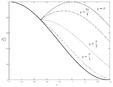
Figure 1: $P^{(1)}_{1,0}\times t$ for different values of $g$.

The strongest inhibition is roused by $g=\pi$ ($\pi$ pulse), which inverts the derivative signal without changing its absolute value. After some algebra we may write the quantum transition rate as:

$$T^{(1)}(t^{(1)}_{m}+t,g=\pi)=\sin(2t^{(1)}_{m}-2t).$$ (18)

The rate is positive ($T^{(1)}(t^{(1)}_{m}+t,g=\pi)>0$) when the evolution time after the interaction with $M$ is smaller than the evolution time before the interaction ($t^{(1)}_{m}>t$). Therefore, the probability $P^{(1)}_{1,0}$ is an increasing function in this interval. For $\frac{\pi}{2}<g<\pi$ the time interval when $P_{1,0}(t)$ is increasing is smaller, that is the reason for the strongest inhibition roused by $g=\pi$.

$N$ sequential measurements

Let us focus on the investigation of a sequence of $N$ interactions between $S$ and $M$ for different values of $g$.

Firstly, we consider interactions that do not entangle the subsystems $S$ and $M$, but rouses meaningful changes on the evolution of $S$ ($g=\pi$).

After, we investigate the possibility of Quantum Zeno Effect with incomplete measurements. We conclude that the enhancement on the number of interactions ($N$) contribute to the decreasing of the quantum transition rate’s absolute value. This is the physical mechanism which allows for the similar behavior between incomplete and complete measurements when $N\rightarrow\infty$.

The dynamics of the system $S$ may be controlled through a sequence of interactions with $g=\pi$.

The modifications induced by a sequence of $N$ $g=\pi$ interactions in $T=N\tau$, where $\tau$ is the time period during which $S$ evolves freely, depends on the parity of $N$. Because at the end of each $g\pi$ interaction the signal of $\frac{dP_{1,0}}{dt}$ is inverted, alternating the behavior of $P_{1,0}(t)$ between increasing and decreasing.

If $N$ is even

$$\prod_{k=1}^{N}\left(U^{k}_{SM}U_{S}\right)|1,0\rangle|0_{M}\rangle=|1,0\rangle|0_{M}\rangle,$$ (19)

and if $N$ is odd

$$\prod_{k=1}^{N}\left(U^{k}_{M}U_{S}\right)|1,0\rangle|0_{M}\rangle=\left(\alpha(\tau)|1,0\rangle+\beta(\tau)|0,1\rangle\right)|0_{M}\rangle.$$ (20)

The control of the dynamics can be achieved from equations (19) and (20). Notice that quantum transition inhibition is more efficient for a sequence of $g=\pi$ interactions than for the traditional QZE.

Figure 2: $P_{1,0}\times N$ for $g=\pi$ (upper curve), $g=\frac{\pi}{2}$(lower curve) and $T=\frac{\pi}{2g}$.

The presence of oscillations in the upper curve is due to the alternate behavior of $P_{1,0}(t)$ (increasing/decreasing) after each $S-M$ interaction. When $N\rightarrow\infty$ the oscillation disappears since the state vector (20) becomes closer and closer to the state in (19).

In order to investigate the modifications on the quantum transition rate induced by a sequence of $N$ interactions between $S$ and $M$ in a fixed time interval, let us consider $T$, divided as shown in Fig 3.

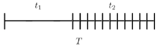
Figure 3: Graphic representation of the time interval $T$ division in $t_{1}$ when $S$ evolves freely and $t_{2}$ interval divided by $N$ interactions between $S$ and $M$.

In $t_{1}$ the system $S$ evolves freely, although, in $t_{2}$ a sequence of $N$ interactions in performed.

If $N\rightarrow\infty$ the time interval between the interactions tend to zero. Therefore, the dynamics becomes very similar to the one in which $N$ consecutive interactions are performed in $t_{2}$. The quantum transition rate after $N$ consecutive interactions in $t_{2}$ can be written as:

$$\frac{dP_{1,0}^{(N)}}{dt}=-2\alpha(t_{1})\beta(t_{1})\cos^{N}(g).$$ (21)

When $N\rightarrow\infty$, $\frac{dP_{1,0}^{(N)}}{dt}\rightarrow 0$. Thus, for a sequence composed of many measurements, the incompleteness of each measurement is an irrelevant factor for the inhibition of the quantum transition. The QZE independs of the intensity of each correlations between $S$ and $M$, the quantum transition rate becomes null in the limit $N\rightarrow\infty$, provided that $|\cos(g)|\neq 1$.

To extend the analysis of the QZE for a finite sequence of incomplete measurements, let us consider the graphics obtained by numerical simulations on Fig 4. The curves show the probability $P_{1,0}$ as function of $N$, for three values of $g$.

In a sequence of incomplete measurements, with $g$ between $\frac{\pi}{2}<g<\pi$, two factors contribute to the inhibition of the transition: derivative’s signal inversion and decreasing of its absolute value.

Let us carefully analise this two factors. At the initial instant the system was prepared in $|1,0\rangle$, as we are investigating the possibility of inhibition of the quantum transition $|1,0\rangle\rightarrow|0,1\rangle$, in the time interval to be considered, the probability $P_{1,0}$ is a decreasing function of the time if no interactions between $S$ and $M$ are performed. After the first measurement (with $\frac{\pi}{2}<g<\pi$), the curve $P_{1,0}\times t$ inverts its behavior and becomes to increase (due to the change on derivative signal), but with the absolute value of transition rate reduced. After the second measurement, the curve $P_{1,0}\times t$ decreases again and the absolute value of the transition rate is even smaller. This effects continues as $N$ increases. The oscillation between increasing and decreasing behavior of $P_{1,0}\times t$, as well as the successive reduction on the absolute value of the transition rate, contribute to the inhibition of the quantum transition.

In measurement sequences with $0<g<\frac{\pi}{2}$ only the reduction on the absolute value of the transition rate contributes to the inhibition of the transition. For this reason in Fig 4, the curve with ($\cos(g)=-0,5$) shows the most rapid increase. When ($\cos(g)=0$) the measurement is complete (traditional QZE) the transition rate becomes null after each measurement. For ($\cos(g)=-0,5$) the interactions induce only the reduction on the absolute value of the transition rate. In the limit $N\rightarrow\infty$ the three curves show the same behavior.

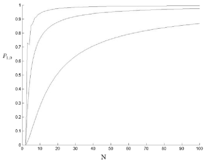
Figure 4: $P_{1,0}\times N$ for $g=\frac{3\pi}{4}$ (upper curve), $g=\frac{\pi}{2}$ (intermediated curve) and $g=\frac{\pi}{4}$ (bottom curve).

To summarize, in the present contribution, we have shown that the QZE persistes even if the entanglement with the measuring probe is not complete. We have also shown that when $\frac{\pi}{2}<g\leq\pi$ the interactions between $S$ and $M$ inhibit the transition in a stronger sense than the traditional QZE.

M.C. Nemes and R. Rossi Jr. acknowledge financial support by CNPq.

References

- (1) B. Misra, E.C. G. Sudarshan, J. Math. Phys. 18, 765 (1977).
- (2) W. M. Itano, D. J. Heinzen, J. J. Bollinger, D. J. Wineland, Phys. Rev. A41, 2295 (1990).
- (3) Wayne M. Itano, arXiv: quant-ph/0612187v1 (2006).
- (4) S. Maniscalco, F. Francica, R. L. Zaffino, N. Lo Gullo and F. Plastina, Phys. Rev. Lett. 100, 090503 (2008).
- (5) P. Facchi, S. Tasaki, S. Pascazio, H. Nakazato, A. Tokuse and D. A. Lidar, Phys. Rev. A71, 022302 (2005).
- (6) P. Facchi, D. A. Lidar and S. Pascazio, Phys. Rev. A69, 032314 (2004).
- (7) Chui-Ping Yang, Shih-I Chu and Siyuan Han, Phys. Rev. Lett. 66, 034301 (2002).
- (8) S. Maniscalco, Jyrki Piilo and Kalle-Antti Suominen, Phys. Rev. Lett. 97, 130402 (2006).
- (9) R. McDermott, R. W. Simmonds, M. Steffen, K. B. Cooper, K. Cicak, K. D. Osborn, Seongshik Oh, D. P. Pappas, J. M. Martinis, Science 307, 1299 (2005).
- (10) Saverio Pascazio, Mikio Namiki, Phys. Rev. A50, 4582 (1994).
- (11) A. F. R. de Toledo Piza and M. C. Nemes, Physics Letters A 290, 6 (2001).
- (12) A. Peres and A. Ron, Phys. Rev. A42, 5720 (1990).
- (13) D. Dhar, L. K. Grover, and S. M. Roy, Phys. Rev. Lett. 96, 100405 (2006).