The rate of secular evolution in elliptical galaxies with central masses

Abstract

We study a series of $N-$body simulations representing elliptical galaxies with central masses. Starting from two different systems with smooth centres, which have initially a triaxial configuration and are in equilibrium, we insert to them central masses of various values. Immediately after such an insertion a system presents a high fraction of particles moving in chaotic orbits, a fact causing a secular evolution towards a new equilibrium state. The chaotic orbits responsible for the secular evolution are identified. Their typical Lypaunov exponents are found to scale with the central mass as a power law $L\propto m^{s}$ with $s$ close to $1/2$. The requirements for an effective secular evolution within a Hubble time are examined. These requirements are quantified by introducing a quantity called effective chaotic momentum $\mathscr{L}$. This quantity is found to correlate well with the rate of the systems’ secular evolution. In particular, we find that when $\mathscr{L}$ falls below a threshold value (0.004 in our $N-$body units) a system does no longer exhibit significant secular evolution.

1 Introduction

Schwarzschild’s (1979) pioneering method confirmed the existence of self-consistent models of elliptical galaxies with exclusively regular orbits (Schwarzschild 1979, 1982; Richstone 1980, 1982, 1984; Richstone & Tremaine 1984; Levison & Richstone 1987). This, together with the study of the perfect ellipsoid model (de Zeeuw & Lyndel-Bell 1985; Statler 1987), which is fully integrable, contributed to the formation of a prevailing aspect during the ’80s that the elliptical galaxies in equilibrium mainly consist of stars moving in regular orbits, while stars in chaotic orbits are either few or inexistent. For this reason galactic dynamical studies were based for many years on a systematic exploration of the stable families of periodic orbits in static galactic potentials.

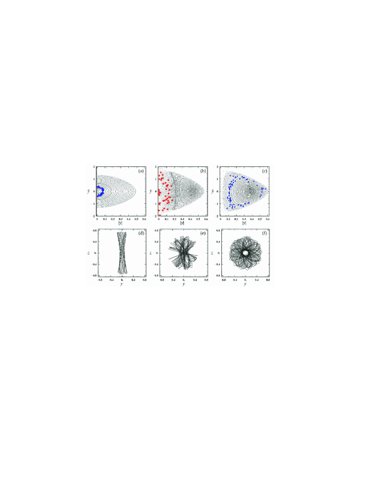
Figure 1: a) The phase portrait (projections on ($|y|,\dot{y}$) of the 4D Poincaré surface of sections ($z=0,\dot{z}>0$)) at an energy level $\simeq 0.74\times$ (the central potential well) in a typical case of our $N-$body simulations (see below), before the insertion of the CM. We see the invariant curves of box orbits. b) The same phase portrait at $t=90T_{hmct}$ after the insertion of the CM. The invariant curves corresponding to box orbits have been destroyed. At their place we have a chaotic domain and an island of regular short axis tube orbits. As the system evolves the chaotic domain is reduced gradually and the island of SAT orbits grows. c) At $t=300T_{hmct}$ after the insertion of the CM, the system has reached its final equilibrium state. The SAT island prevails. In each of these panels blue dots correspond to regular motion while red stars correspond to chaotic motion of one of the $N-$body particles. d) Before the insertion of the CM the particle moves in a box orbit. e) For $t=0-180T_{hmct}$ after the insertion of the CM the particle wanders in the chaotic domain. f) After $t\simeq 180T_{hmct}$ the particle is trapped by SAT tori and its orbit is converted to regular, of the SAT type.

This point of view was challenged in the early ’90s when Schwarzschild (1993) found that chaos plays a significant role in the structure of systems with cuspy density profiles $(\rho_{halo}\propto r^{-2})$. A number of observations also indicated that high values of Central Masses (CM) exist in galaxies (Crane et al. 1993; Ferrarese et al. 1994; Lauer et al. 1995; Kormendy & Richstone 1995; Gebhardt et al. 1996; Faber et al. 1997; Kormendy et al. 1997, 1998; van der Marel et al. 1997; van der Marel & van den Bosch 1998; Magorrian et al. 1998; Cretton & van den Bosch 1999; Gebhardt et al. 2000). Gerhard & Binney (1985) had shown how box orbits are converted to chaotic orbits in systems with strong CM. Later, many authors studied in detail this phenomenon and its consequences for elliptical galaxies (Merritt & Fridman 1996; Merritt & Valuri 1996, 1999; Fridman & Merritt 1997, Valluri & Merritt 1998; Merritt & Quinlan 1998; Siopis 1999, Siopis & Kandrup 2000; Holley Bockelmann et al. 2001, 2002; Poon & Merritt 2001, 2002, 2004; Kandrup & Sideris 2002; Kandrup & Siopis 2003; Kalapotharakos, Voglis & Contopoulos 2004; Kalapotharakos & Voglis 2005, see Merritt 1999, 2006 and Efthymiopoulos, Voglis & Kalapotharakos 2007 for a review). In particular, using the Schwarzschild’s method Merritt & Fridman (1996) found self-consistent solutions for triaxial configurations in the case of a weakly cuspy profile $\rho\propto r^{-1}$. In these solutions the fraction of particles in chaotic orbits raised up to $\simeq 46\%$. On the other hand, in the case of strongly cuspy profiles $\rho\propto r^{-2}$ the optimal solutions found had $\simeq 60\%$ chaotic orbits. However, the solutions in the latter case were not fully stationary.

It should be noted that, while a solution of the Schwarzschild method should ideally represent a stationary galaxy, in practice an $N-$body realization of such a solution will show some secular evolution due to a number of reasons, namely a) the solution’s response density may not match precisely the imposed density b) some of the chaotic orbits of the solution may not be ‘fully mixed’ i.e. they may have not reached a full covering of their invariant measure in the phase space within the method’s fixed integration time, and c) by its nature Schwarzschild’s method cannot secure the stability of even a perfect solution. Thus, questions related to the stability or secular evolution of a self-consistent model of a galaxy are better answered by the $N-$body method, which is free of the limitations of Schwarzschild’s method.

Many works by the $N-$body method have addressed the questions of the orbital analysis and of the relation between the self-consistency and the orbital content of either stationary or evolving systems (Holley-Bockelmann et al. 2001, 2002; Contopoulos, Voglis & Kalapotharakos 2002; Voglis, Kalapotharakos & Stavropoulos 2002; Kalapotharakos et al. 2004; Kalapotharakos & Voglis 2005; Muzzio, Carpintero & Wachlin 2005; Jesseit, Naab & Burkert 2005; Muzzio 2006; Voglis, Stavropoulos & Kalapotharakos 2006). In these works it has been repeatedly demonstrated that the insertion of a CM in a triaxial system at equilibrium leads to significant secular evolution, resulting in a new equilibrium state which is, in most cases oblate (Merritt & Quinlan 1998; Holley-Bockelmann et al. 2001, 2002; Kalapotharakos et al. 2004; Kalapotharakos & Voglis 2005).

Kalapotharakos et al. (2004), Kalapotharakos & Voglis (2005) extended the research of Voglis et al. (2002) for a series of models with CMs. These works unravelled very clearly the transformation of the phase space during the secular evolution that leads the systems to a new equilibrium state. A summary of our previous results, needed in the sequel, can be made with the help of Fig. 1. Fig. 1a shows the phase space structure in an example of our simulations before the insertion of the CM. The phase portrait is almost entirely filled by invariant curves corresponding to box orbits. The big blue dots correspond to the Poincaré consequents of a specific particle’s orbit (called hereafter particle A). Note, that these dots are provided by the self-consistent $N-$body run. After the insertion of the CM practically all the tori of box orbits are destroyed and their place is occupied by a chaotic domain and by smaller islands corresponding to the well known ‘boxlets’ (e.g. Merritt 1999; these orbits were called High Order Resonant Tube (HORT) in previous works of ours). Now, as the chaotic orbits diffuse in the phase space they cause a secular change of the system’s form, which becomes more spherical and less prolate. This change, on its turn, affects the phase space favouring Short Axis Tube (hereafter SAT) orbits. Fig. 1b shows the phase space structure (black points) at $t=90$ half mass crossing times (hereafter $T_{hmct}$). We observe a large chaotic domain (for $|y|\lesssim 0.2$) and a big island of stability (for $|y|\gtrsim 0.2$) corresponding to SAT orbits. Note, that in the present paper we always consider the half mass radius $R_{h}$ being equal to unity ($R_{h}=1$). The red stars correspond to the Poincaré consequents of the orbit of particle A in the time interval $t=0-180T_{hmct}$. The main effect is the following: As the island of SAT orbits grows, the majority of particles, initially in chaotic orbits, are gradually trapped in the domain of SAT tori and the orbits are converted to regular, of the SAT type. Fig. 1c shows this conversion for particle A. The second row of Fig. 1 shows also the gradual conversion of the same orbit from box to chaotic and then to SAT, as it appears in ordinary space. The phase space structure in Fig. 1c corresponds to $t=300T_{hmct}$ (a Hubble time) and the big blue dots correspond to the consequents of the orbit of particle A within the time interval $t=180-350T_{hmct}$. At $t=300T_{hmct}$ the system has already reached its final equilibrium state. At this snapshot the number of particles in chaotic orbits is considerably lower than at $t=0$.

In the systems studied by Kalapotharakos et al. (2004) the destruction of box tori after the insertion of the CM results in the fraction of mass in chaotic orbits rising initially up to the level of $50\%-80\%$ (depending on the initial maximum ellipticity of the system). However, during the secular evolution of these systems the fraction of chaotic orbits decreases significantly and at the new equilibrium state this fraction ranges between $\simeq 10\%$ and $\simeq 25\%$. The rate of secular evolution depends on the mass value of the CM as well as on the configuration of the original system before the insertion. In particular, different mass values lead not only to different fractions of particles in chaotic orbits, but also to different distributions of the particles’ Lyapunov exponents.

In the present paper our goals are:

a) to study the relation between the mass value of the CM, on the one hand, and the corresponding values of the Lyapunov characteristic exponents, on the other hand, of those chaotic orbits which are produced due to the insertion of the CM and are responsible for the secular evolution. We can immediately state the result of this investigation, which constitutes one principal result of the present paper: we find that this relation is a power law with an exponent close to $1/2$. Work on the theoretical justification of such a scaling law is in progress, but a preliminary discussion is given in the final section of the paper.

b) to determine the specific requirements so that a system exhibits significant secular evolution within a Hubble time. Surprisingly, it was found that, independently of the details of a system, the onset of significant secular evolution takes place when a quantity termed effective chaotic momentum surpasses a threshold value (equal to 0.004 in the present paper’s $N-$body units). This threshold is global, i.e. the same for all the studied systems. This indicates that the effective secular momentum is a quantity possibly related to a more fundamental statistical mechanical description of the systems under study.

Section 2 briefly describes the models. Section 3 discusses the relation between the value of the CM and the characteristic values of the Lyapunov exponents of its associated chaotic orbits. Section 4 contains the definition of the effective chaotic momentum, that measures the ability of a system to undergo secular evolution within a Hubble time. Finally, section 5 summarizes the main conclusions of the present study.

Table 1: The fractions of the total number of particles in chaotic orbits in the various systems for $t=0$ (the moment when the CM is inserted).

models	$m=0$	$m=0.0005$	$m=0.001$	$m=0.005$	$m=0.01$
Q	32%	79%	82%	81%	80%
C	23%	48%	51%	53%	50%

Table 2: The fractions of the total number of particles in chaotic orbits in the various systems for $t=150T_{hmct}$ (half a Hubble time).

models	$m=0$	$m=0.0005$	$m=0.001$	$m=0.005$	$m=0.01$
Q	32%	78%	80%	73%	56%
C	23%	47%	48%	40%	30%

Table 3: The fractions of the total number of particles in chaotic orbits in the various systems at the final equilibrium state.

models	$m=0$	$m=0.005$	$m=0.01$
Q	32%	25% (at $t=300$)	22% (at $t=2200$)
C	23%	19% (at $t=2200$)	12% (at $t=2200$)

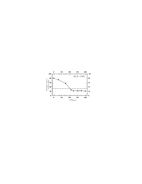
Figure 2: The evolution of the percentage of chaotic orbits in the system (Q, $m=0.01$). Initially, we have a high percentage ($\simeq 80\%$) of chaotic orbits that decreases with time. When the system reaches the final oblate equilibrium state the percentage of chaotic orbits remains stabilized at a level $\simeq 20\%$. The horizontal dashed line denotes the percentage of chaotic orbits in the Q system (before the insertion of the CM).

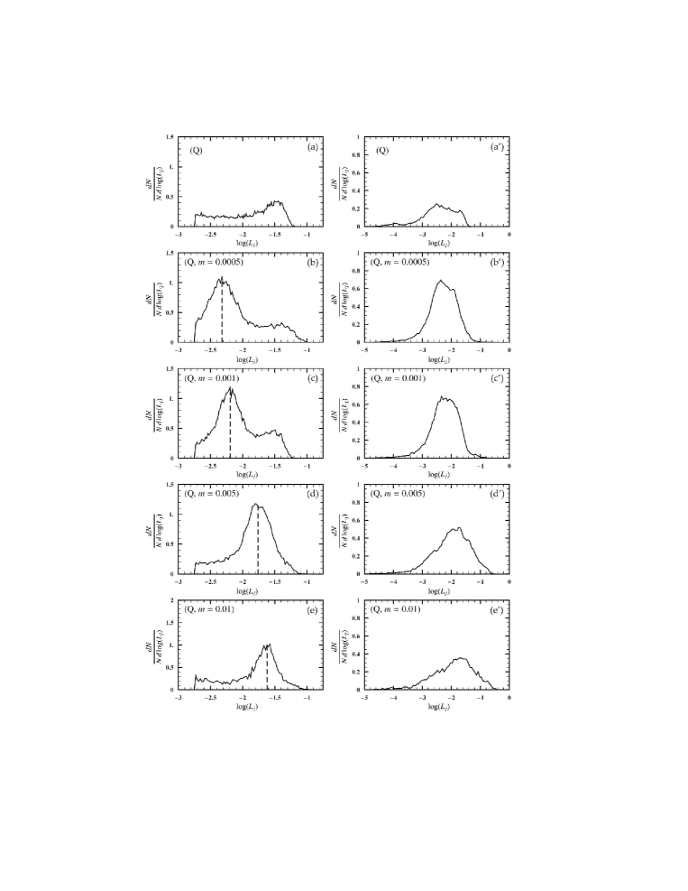
Figure 3: Left column: The distributions of $\log(L_{j})$ for the chaotic orbits of the Q family systems at the snapshot $t=150T_{hmct}$, with mass parameters $m$ as indicated in the panels. A pronounced maximum appears for the systems with $m\neq 0$, which is shifted towards higher values of $\log(L_{j})$ as $m$ increases. Note, that the area below each curve denotes the corresponding function of chaotic orbits. Right column: Same as in the left column for the distributions of $\log(L_{cuj})$.

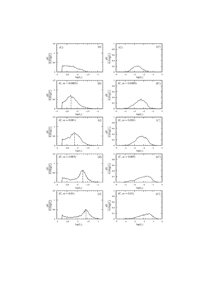
Figure 4: Same as in Fig. 3 but for the C family systems.

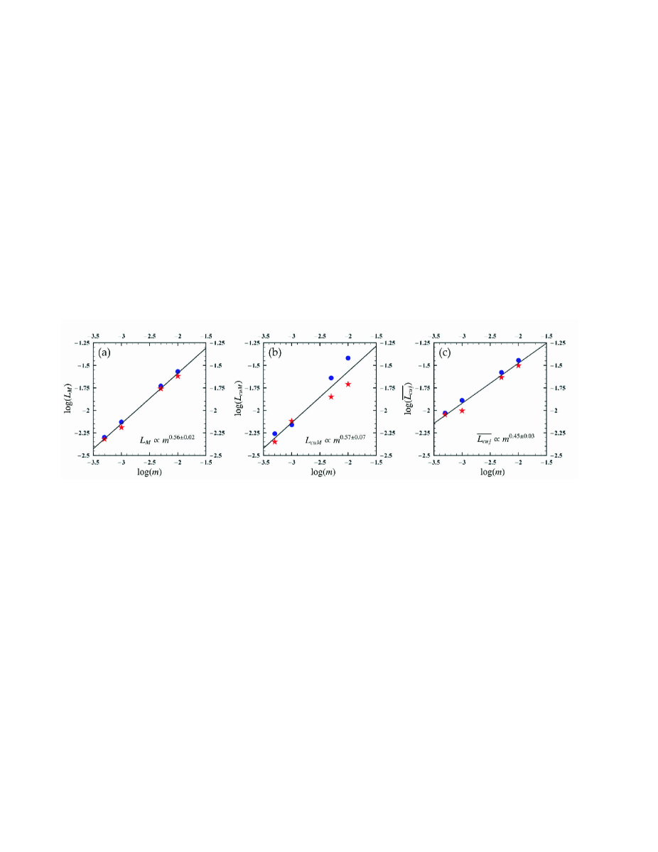
Figure 5: The values of a) $\log(L_{M})$, b) $\log(L_{cuM})$ and c) $\log(\overline{L_{cuj}})$ against $\log(m)$. Red stars and blue dots correspond to the Q and C family systems respectively. All three Lyapunov numbers $-~{}\log(L_{M})$, $\log(L_{cuM})$, $\log(\overline{L_{cuj}})~{}-$ are well fitted by power laws $\propto m^{s}$ with exponents s near the value 0.5.

2 Description of the models

Our study refers to the insertion of a CM in a variety of equilibrium $N-$body systems. The latter are described in detail in Kalapotharakos et al. (2004). Here we describe briefly the most important features of these systems.

Two families of models are examined in the present paper. They are produced from two different original systems representing smooth centre elliptical galaxies in equilibrium. The two initial systems are both triaxial, but nearby prolate. The first system (called Q system) has a maximum ellipticity $E_{max}\simeq 7$ and triaxiality $\simeq 0.9$ while the second system (called C system) has a maximum ellipticity $E_{max}\simeq 3.5$ and triaxiality $\simeq 0.8$. Note that the short, intermediate and long axes of each system in the present study is aligned along the $x,y,z$ axes, respectively. Voglis et al. (2002) calculated the fractions of particles moving in chaotic orbits in these systems. They found $\simeq 32\%$ and $\simeq 23\%$ for the Q and C system, respectively. These fractions, as well as the identities of the particles moving in chaotic orbits, remain almost unchanged in time, before the insertion of the CM.

We insert, in these systems, CMs with a variety of mass values and follow numerically their evolution by the $N-$body code (Allen, Palmer & Papaloizou 1990). We then calculate the fractions of the particles moving in chaotic orbits at various snapshots of this evolution. The CM is assumed to have the following density profile (Allen et al. 1990):

$$\rho_{cm}=\dfrac{GM_{cm}a^{2}}{2\pi r(r^{2}+a^{2})^{2}}$$ (1)

where $a=0.005mR_{g}$, $m=\dfrac{M_{cm}}{M_{g}}$ is the relative value of the CM with respect to the total galaxy mass $M_{g}$, and $R_{g}$ is the radius of galaxy. The profile (1) yields a cuspy profile $r^{-1}$ for $r\ll a$. We examined four different values of $m$, namely $(0.0005,0.001,0.005,0.01)$.

The fraction of mass in chaotic motion, corresponding to the integration of orbits in a ‘frozen’ potential of each system at the snapshot $t=0$ (the moment when the CM is inserted), is approximately $80\%$ in all the Q models (for various masses $m$), and approximately $50\%$ in all the C models. These percentages turn to be rather irrelevant to the values of $m$ considered (Table 1).

In subsequent (isochronous) snapshots, these fractions are seen to vary for different values of $m$. Table 2 shows the fractions of particles detected in chaotic orbits at the time $t=150T_{hmct}$ (half a Hubble time) after the insertion of the CM. The main remark with respect to this table is that, the systems with higher values of $m$ (0.005, 0.01) exhibit smaller fractions of chaotic orbits than the systems with lower values of $m$ (0.0005, 0.001) which retain a fraction of chaotic orbits almost equal to the fractions at the snapshot $t=0$ (compare Tables 1 and 2).

Now, Table 3 shows the fractions of the chaotic orbits for the systems with high values of $m$ (0.005, 0.01), when the systems have reached a new equilibrium state. The main observation here is that in all cases the fraction of chaotic orbits at the new equilibrium state is far smaller than the fraction of the chaotic orbits in the same system at $t=0$ (compare Tables 1 and 3). In fact, the final fraction is even smaller than the fraction of chaotic orbits in the same systems before the insertion of the CM. In Fig. 2 we see, for example, the evolution of the fraction of chaotic orbits for the system (Q, $m=0.01$). The gradual decrease of this fraction is shown clearly up to the moment when the system reaches the new oblate equilibrium state ($t\simeq 220$). In the case of systems with low values of $m$ the corresponding fractions were not calculated because these systems need much longer intervals than a Hubble time to reach an equilibrium. For example, after a period of 20 Hubble times the $m=0.001$ system of the Q family appears to be still far from equilibrium (see fig. 4 of Kalapotharakos et al. 2004). The times (in $T_{hmct}units$) of final states of all the systems that have reached a final equilibrium state is given in Table 3, for comparison.

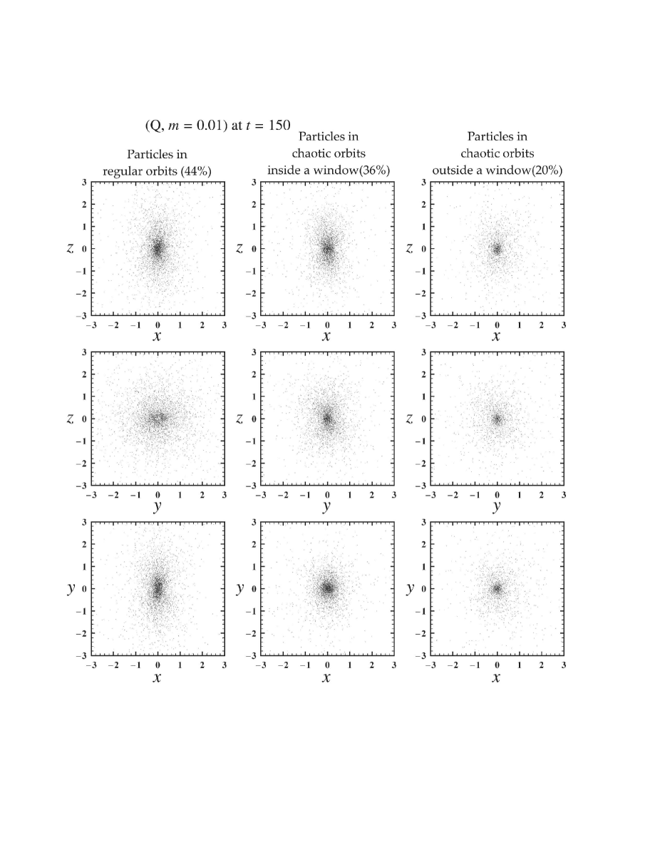
Figure 6: Each column shows the projections of different mass components of the (Q, $m=0.01$) system on the three principal planes ($x-z,~{}y-z,~{}x-y$) at $t=150T_{hmct}$. Left column: Projection of the particles in regular orbits. These particles constitute approximately $44\%$ of the total mass and they form a strongly flattened (oblate) configuration. The orbits are mainly of SAT and boxlet (called ‘HORT’ in Kalapotharakos & Voglis 2005, see text) type. Middle column: Projection of the particles in chaotic orbits with $L_{j}$s within a window located around the maximum $\log(L_{M})$ of the distribution of Fig. 3e. These particles constitute approximately $36\%$ of the total mass. They form a triaxial configuration and they were moving in box orbits before the insertion of the CM. After the insertion, they are responsible, through their chaotic diffusion, for the secular evolution exhibited by the system. Right column: Projection of the particles in chaotic orbits with $L_{j}$s outside the window around the $\log(L_{M})$ maximum. This component constitutes approximately $20\%$ of the total mass and it forms an isotropic (spherical) configuration. The spherical distribution is due to the nearly complete mixing of the particles in the phase space due to chaotic diffusion. Such particles no longer contribute to the systems’s overall secular evolution.

3 CM and Lyapunov exponents

In order to distinguish the orbits into regular and chaotic we use two indices: a) The Specific Finite Lyapunov Characteristic Number or $L_{j}$ and b) the Alignment Index (AI) or Smaller ALignment Index (SALI) (for more details see Voglis, Contopoulos & Efthymiopoulos 1998; Voglis, Contopoulos & Efthymiopoulos 1999; Skokos 2001; Voglis et al. 2002). The $L_{j}$ has as unit the inverse of the radial period of each orbit $T_{rj}$ and provides a good answer regarding whether an orbit can be characterized as regular or chaotic (up to a certain level). It can also provide a comparison of the relative degree of chaos of two orbits provided that their $L_{j}$s have already reached a stabilized value within a given integration time. However, since the $L_{j}$ is measured by a different unit for each orbit, it cannot be used for a comparison of the orbits as regards the efficiency of their chaotic diffusion in phase space. For this reason, the $L_{j}$s are converted to quantities with a common unit for all the particles. The Common Unit Finite Time Lyapunov Characteristic Number or simply $L_{cuj}$ is defined by

$$L_{cuj}=L_{j}\dfrac{T_{hmr}}{T_{rj}}$$ (2)

in units $1/T_{hmr}$, where $T_{hmr}$ is the period of radial oscillations of the orbits with energy equal to the value of the potential at a radius equal to the half-mass radius $R_{h}$. One finds $T_{hmr}\simeq 3T_{hmct}$. This Lyapunov exponent $L_{cuj}$ compares the chaotic orbits with respect to their ability to undergo significant chaotic diffusion within a Hubble time. In summary, the value of $L_{j}$ gives us a measure of the overall complexity and chaoticity of the phase space inside which the orbits lie, while the value of $L_{cuj}$ yields the exponential rate of deviation, measured in absolute time units for each individual orbit.

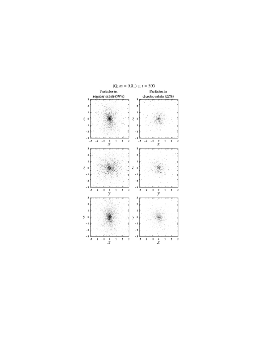
Figure 7: Left column: The projections of the particles in regular orbits of (Q, $m=0.01$) system on the three principal planes at $t=300T_{hmct}$. These particles constitute $78\%$ of the total mass and form an oblate configuration. Right column: The same projection of the particles moving in chaotic orbits. These particles constitute $22\%$ of the total mass and form an almost spherical configuration. The chaotic diffusion does no longer have any consequences on the form of the system.

Now, Fig. 3 shows the distributions of the values of $\log(L_{j})$ axis (left column) or the values of $\log(L_{cuj})$ (right column) at the snapshot $t=150T_{hmct}$ for the particles in chaotic orbits of all the systems of the Q family. The distributions are normalized with respect to the systems’ fraction of chaotic orbits, i.e., the area below each curve denotes the fraction of chaotic orbits. The following are observed:

a) All the distributions of the values of $\log(L_{j})$ for $m>0$ (Fig. 3 - left column) exhibit a global maximum at values $\log(L_{j})=\log(L_{M})$. For $m=0$ (Fig. 3a) there appears no conspicuous maximum. On the other hand, for $m>0$ there appears a conspicuous maximum which is, furthermore, shifted to the right as $m$ increases. By examining many orbits with $L_{j}$s in an interval around these maxima we found that such orbits correspond to particles that were initially moving in box orbits (before the insertion of the CM).

b) The distributions of the values of $\log(L_{cuj})$ axis (Fig. 3 - right column) are quite different from the corresponding distributions of $\log(L_{j})$. Nevertheless, these distributions also exhibit global maxima, at values $\log(L_{cuM})$ not very different from $\log(L_{M})$.

Similar remarks can be made for the systems of the C family (Fig. 4). It is clear from Figs. 3 and 4 that the values $\log(L_{M})$ and $\log(L_{cuM})$ (for $m\neq 0$) depend on $m$. The mean value of $L_{cuj}$, denoted by $\overline{L_{cuj}}$, also depends on $m$. The main result now, is that all the three dependencies are power laws functions of $m$ (Fig. 5). In Fig. 5, the red stars refer to the systems of the Q family and the blue dots to the systems of the C family. The power laws of $L_{M}$ (Fig. 5a), $L_{cuM}$ (Fig. 5b) and $\overline{L_{cuj}}$ (Fig. 5c) are

$$L_{M}\propto m^{s_{1}}$$ (3a)

$$L_{cuM}\propto m^{s_{2}}$$ (3b)

$$\overline{L_{cuj}}\propto m^{s_{3}}$$ (3c)

where $s_{1}=0.56\pm 0.02,~{}s_{2}=0.57\pm 0.07$ and $s_{3}=0.45\pm 0.03$. The quantities $L_{M}$, $L_{cuM}$ and $\overline{L_{cuj}}$ are different measures of the mean level of the Lyapunov exponents of the orbits, which have become chaotic, precisely by the insertion of the CM. In conclusion, the Lyapunov characteristic exponents of the chaotic orbits scale approximately as $m^{1/2}$. This property appears here as a numerical result, but it probably has some theoretical explanation related to the scattering of the orbits by the CM near the centre (see discussion).

4 Effective chaotic momentum

In Fig. 5 we see that the systems with $m<0.0050$, have an $\overline{L_{cuj}}$ close to the value $10^{-2}$. These systems do not exhibit appreciable evolution within a Hubble time. On the other hand, the systems with $m\geq 0.0050$, develop a well detectable secular evolution within a Hubble time. In that case the $\overline{L_{cuj}}$ values are close to $10^{-1.5}$. In a first approximation, we can say that this difference between the mean Lyapunov exponents of the systems with low or high central mass value $m$ can explain the faster evolution rate in the latter case, since the diffusion of a chaotic orbit is effective within a Hubble time ($\sim 100T_{hmr}$) only when its $L_{cuj}$ value is $L_{cuj}\gtrsim 10^{-2}$.

However, a more careful study revealed two basic requirements which must be fulfilled in order for a system to undergo significant secular evolution within a Hubble time:

1. the fraction of mass in chaotic motion with high $L_{cuj}$ values ($L_{cuj}>10^{-2}$) must not be very small and

2. this mass must have an anisotropic initial distribution in ordinary space. In fact, whenever the mass appears isotropically distributed (i.e. close to a spherical distribution) this is an indication that the chaotic mixing has already taken place in the phase space, i.e. the particles in chaotic orbits have already acquired an almost uniform distribution in the phase space. We should stress that a spherical distribution of the particles in chaotic motion is not incompatible with the appearance of chaos itself, since the particles in regular orbits provide a significant perturbation of the overall galactic potential from a spherical potential.

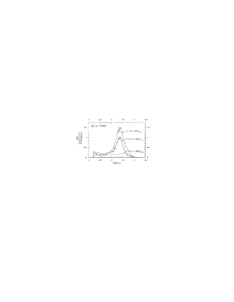
Figure 8: The distribution of $\log(L_{j})$ for the particles in chaotic orbits of the system (Q, $m=0.01$) at three different times a) $t=0$, b) $t=150T_{hmct}$ c) $t=300T_{hmct}$. The mass converted from chaotic to regular orbits during the secular evolution comes mainly from the area around the global maximum.

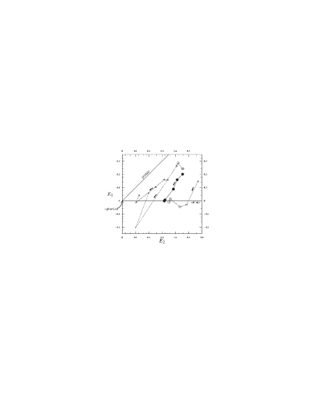
Figure 9: The time evolution of the various populations of the system (Q, $m=0.01$) on the plane of the ellipticities $(E_{2},E_{1})=(1-\frac{a}{c},1-\frac{b}{c})$, where $a,b,c$ are the short, intermediate and long axes respectively as calculated by the moment of inertia tensor of each population. The black dots correspond to the system (Q, $m=0.01$) as a whole, the white circles correspond to the regular component and the rectangles and the triangles correspond to the chaotic component inside and outside of the window of the $\log(L_{j})$ distribution, respectively. The total area within each symbol represents the percentage of the associated population with respect to the total number of particles. The small arrow in each curve indicates the time arrow. The five snapshots that are plotted are at $t=(0,60,150,300,600)T_{hmct}$. We observe that all the different populations exhibit an overall evolution towards a more oblate configuration ($E_{1}=0$). However, the regular component is always far from a spherical distribution (corresponding to $E_{1}=E_{2}=0$), while the latter is more closely approached from the start by the chaotic orbits outside the window.

In order to identify which particles in chaotic motion are most responsible for the secular evolution of the systems, we collected the particles with $\log(L_{j})$ values in the window $\log(L_{M})-0.3\leq\log(L_{j})\leq\log(L_{M})+0.3$ in Figs. 3 and 4, i.e., the particles within roughly one dispersion interval around the maxima of each distribution. The majority of the particles inside this window are found to be particles moving mainly in box orbits in the corresponding smooth centre system before the insertion of the CM. Up to $t=150T_{hmct}$ these particles preserve to a large extend their initial, strongly non spherical, distribution. For example, Fig. 6 shows the distributions of the particles in regular and in chaotic orbits for the system (Q, $m=0.01$) at the snapshot $t=150T_{hmct}$. The left column shows the projections of the particles in regular orbits on the three principal planes $x-z$, $y-z$ and $x-y$ as indicated in the panels. According to Table 2 these particles constitute $44\%$ of the total mass of the system. This component forms a nearly oblate configuration. The middle column shows similar projections, but for the particles lying inside the $\pm 0.3$ window around the value $\log(L_{M})=10^{-1.62}$ of Fig. 3e. This mass constitutes approximately $36\%$ of the total mass and has a triaxial strongly elongated configuration. On the other hand, the right column shows the distribution for the remaining particles in chaotic orbits (outside the corresponding window). This mass, which constitutes approximately $20\%$ of the total mass, creates an almost spherical background.

The source of secular evolution of the system (Q, $m=0.01$) is the mass (in chaotic motion) of the middle column. During the evolution, the majority of the particles’ orbits become regular, mainly SAT orbits (Kalapotharakos et al. 2004; Kalapotharakos & Voglis 2005). The particles remaining in chaotic orbits form finally an almost spherical distribution. This appears in Fig. 7 which shows the particles in regular or chaotic orbits in the same system but for the snapshot $t=300T_{hmct}$. The particles in regular orbits constitute approximately $78\%$ of the total mass (left column). At this time the system has already settled down to a nearly oblate equilibrium state. It is immediately observed that the particles in regular orbits (left column) support the form of an oblate spheroid, while the particles in chaotic orbits (right column) form an almost spherical distribution.

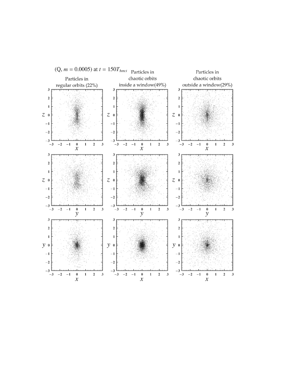
Figure 10: Similar to Fig. 6 but for the (Q, $m=0.005$) system. The regular component (left column) constitutes $\simeq 22\%$ of the total mass and forms a strongly elongated structure. The part of the chaotic component that lies around the maximum of the distribution of Fig. 3b (middle column) constitutes $\simeq 49\%$ of the total mass and has a very similar configuration to that of regular component. The chaotic diffusion of this mass is mainly responsible for the secular evolution. The remaining part of the chaotic component (right column) has a much more uniform and isotropic configuration. These orbits are already mixed in their available phase space.

Now, fig. 12 in Kalapotharakos et al. (2004) gives already a hint that the orbits converted, during the secular evolution, from chaotic to regular belong to the domain of the distributions of $\log(L_{j})$ near the maximum. Fig. 8 shows a comparison of the distributions of $\log(L_{j})$ for the mass in chaotic orbits of the system (Q, $m=0.01$) for three different snapshots, namely $t=0$ (dotted-dashed line), $t=150T_{hmct}$ (solid line) and $t=300T_{hmct}$ (dotted line). The area below each curve corresponds to the fraction of the mass in chaotic orbits at each snapshot. The clear maximum appearing at $\log(L_{M})=10^{-1.62}$ of the first distribution (at $t=0$) is smaller in the second distribution (at $t=150T_{hmct}$) and even smaller (but still detectable) in the last distribution (at $t=300T_{hmct}$) at the position $\log(L_{M})\simeq 10^{-1.5}$. The decrease of this maximum implies that many chaotic orbits were converted gradually to regular orbits. Such conversions drive the secular evolution of the system, and they are produced mainly from particles in the area of this maximum.

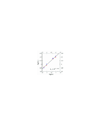
Figure 11: $\log(L_{w})$ and $\log(m)$ are related through the power law $L_{w}\propto m^{0.57\pm 0.2}$.

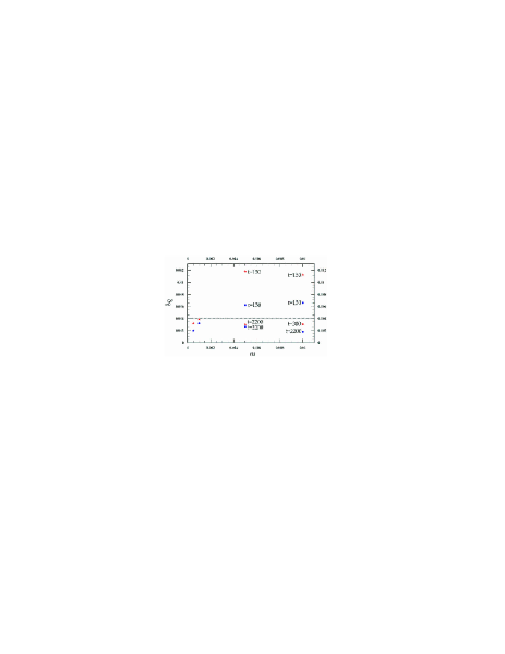
Figure 12: The effective chaotic momentum $\mathscr{L}$ versus $m$. The red stars correspond to the Q family systems and the blue dots correspond to the C family systems. In the case of systems showing negligible secular evolution within a Hubble time one point is plotted for the value of $\mathscr{L}$ at the time $t=150T_{hmct}$. In the case of systems showing detectable secular evolution within a Hubble two points are plotted corresponding to $t=150T_{hmct}$ and to the equilibrium state. The systems showing negligible or no secular evolution have $\mathscr{L}$ values lower than $\simeq 0.004$. The systems with detectable secular evolution ($m=0.005,~{}m=0.01$) have initially high $\mathscr{L}$ values ($\mathscr{L}>0.004$) and finally low $\mathscr{L}$ values ($\mathscr{L}<0.004$).

Figure 9 shows how does the distribution of particles in different types of orbits affect the geometric parameters, i.e. ellipticity and triaxiality, of the $(Q,m=0.01)$ system, in the course of the latter’s secular evolution. This figure is produced by calculating the time evolution of the moment-of-inertia tensor of the $(Q,m=0.01)$ system as a whole, and separately for the regular orbits, the chaotic orbits within the main window of the $\log(L_{j})$ distribution, and the chaotic orbits outside this window. The plot shows the ellipticity $E_{1}=1-b/c$ (vertical axis) versus $E_{2}=1-a/c$ (horizontal axis), where a,b,c are the short, intermediate and long axes respectively as calculated by the moment of inertia tensor of all the particles of the system (black circles). The white circles correspond to the same quantities for regular orbits, the squares to chaotic orbits within the main window of the $\log(L_{j})$ distribution, and the triangles to chaotic orbits outside the main window. The total area within a circle, square or triangle symbol is proportional to the percentage of the associated population with respect to the total number of particles. The five points per curve correspond to five different time snapshots as indicated in the figure. Clearly, the overall evolution of the system is towards an oblate state (corresponding to the straight line $E_{1}=0$). All the different populations exhibit an overall evolution towards a more oblate configuration. We notice, however, that the regular orbits are always far from a spherical distribution (corresponding to $E_{1}=E_{2}=0$), while the latter is more closely approached from the start by the chaotic orbits outside the main window. This further substantiates the phenomena described so far in Figs. 6 and 7. In particular, the chaotic diffusion causes the orbits inside the main window to fill the entire phase space available to them. In the configuration space, this implies that the chaotic orbits of any given constant energy fill progressively a larger and larger volume within the equipotential surface corresponding to that energy (this is in contrast to the box or tube orbits which only fill boxes or tubes in such a volume). Furthermore, in typical galactic potentials the equipotential surfaces are rounder than the surfaces of equal density. Thus, the chaotic diffusion causes the spatial distribution of the orbits within the main window to become more and more spherical and this is the main factor driving the secular evolution.

In order to demonstrate that the maxima of the distributions of (Figs. 3, 4) are important as regards the secular evolution of the systems, Fig. 10 shows a plot similar to Fig. 6, but for the system (Q, $m=0.0005$) at the snapshot $t=150T_{hmct}$. The particles in regular orbits shown in the left column constitute approximately $22\%$ of the total mass and form a triaxial strongly elongated configuration, which consists mainly of SAT orbits and boxlets that have survived after the insertion of the CM. The particles in chaotic orbits which are inside the window $(\pm 0.3)$ around the value $\log(L_{M})=10^{-2.32}$ (Fig. 3b) constitute approximately $49\%$ of the total mass (middle column of Fig. 10). The spatial distribution of this mass is quite similar to that of the mass of the left column. The right column shows the projections of the particles in chaotic orbits with values of $\log(L_{j})$ outside the $\pm 0.3$ window (approximately $29\%$ of the total mass). These particles form a more isotropic distribution compared to these of the left and middle columns in the same figure. Because of the low values of $\log(L_{M})$, the rate of chaotic diffusion of the particles in the middle column is so slow that a macroscopic secular evolution was not detected even for times much longer than a Hubble time.

In conclusion, the rate of secular evolution of the systems depends mainly on the fraction of particles in chaotic orbits which are distributed anisotropically (strongly non spherical) and on the mean value of the Lyapunov exponents $L_{cuj}$ of the same orbits, which measures the ability for chaotic diffusion.

The fraction of anisotropically distributed mass in chaotic motion can be derived by the ratio $\dfrac{\Delta N_{w}}{N_{total}}$, where $\Delta N_{w}$ is the mass inside the window around the maximum of the $\log(L_{j})$ distributions in Figs. 3 and 4 and $N_{total}$ is the total number particles in the system. If, now, the mean value of $L_{cuj}$ for the mass inside this window is $L_{w}$, a measure of the efficiency of the chaotic diffusion can be obtained by the quantity

$$\mathscr{L}=\dfrac{\Delta N_{w}}{N_{total}}L_{w}$$ (4)

hereafter called effective chaotic momentum. The physical motivation behind the characterization of $\mathscr{L}$ as a ‘momentum’ is that the quantity $L_{w}$ represents a ‘speed’, i.e. the speed of growth of deviations in the tangent space to the phase space of the particles’ motion, while this speed is multiplied by a mass $\Delta N_{w}$, i.e., the total mass of the particles in chaotic orbits causing substantial chaotic diffusion.

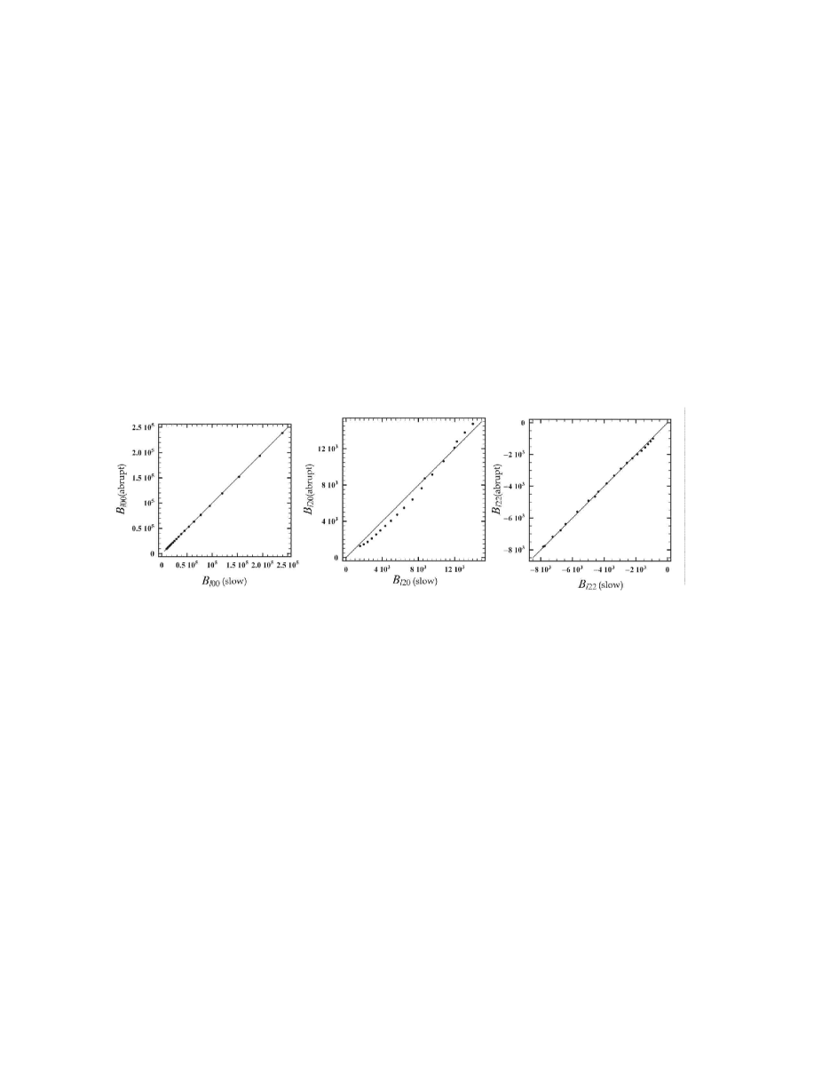
Figure 13: A comparison of values of the most important coefficients ($B_{l00},B_{l20},B_{l22},~{}l=0...19$) of the multipole expansion of the potential (see eq. 13 of Kalapotharakos et al. 2004) of the final equilibrium state of the system (Q $m=0.01$) when the introduction of the CM is done slowly (values in the horizontal axis) or abruptly (values in the vertical axis). The points in these diagrams lie close to the diagonal, meaning that the final states derived by the two simulations are almost the same.

Now, Fig. 11 shows the value of $\log(L_{w})$ versus $\log(m)$ for all the experiments. A power law fit $L_{w}\propto m^{s}$ with $s=0.57\pm 0.02$ is found, which is similar to the power laws found in the previous section. On the other hand, the relation between $\mathscr{L}$ and the rate of systems’ evolution is shown in Fig. 12. The red stars correspond to the systems of the Q family while the blue dots correspond to the systems of the C family. For those systems exhibiting detectable secular evolution within a Hubble time, i.e. the Q and C systems with $m=0.005$ or $m=0.01$, the figure shows two points per system corresponding to measurements of $\mathscr{L}$ at two different snapshots namely $t=150T_{hmct}$ and $t$ equal to time when a system reaches its final equilibrium state (as indicated in the figure). For the systems with low values of the CM, Fig. 12 shows only one point corresponding to the value of $\mathscr{L}$ at the snapshot $t=150T_{hmct}$.

Figure 12 shows that $\mathscr{L}$ is a good measure of the rate of secular evolution. For example, at $t=150T_{hmct}$ the system (Q, m=0.001) has a very high fraction of chaotic orbits ($80\%$), but the majority of these orbits have low values of Lyapunov exponents (Figs. 3c,c^′). On the other hand, at the same time the system (C, $m=0.01$) has a much smaller fraction of chaotic orbits ($30\%$) but the majority of them have high values of Lyapunov exponents (Figs. 4e,e^′). Thus, the $\mathscr{L}$ value of the system (C, $m=0.01$) is higher than the $\mathscr{L}$ value of the system (Q, $m=0.001$), In accordance with that, the system (C, $m=0.01$) has a much faster rate of secular evolution than the system (Q, $m=0.001$). In the case of systems not showing detectable secular evolution within a Hubble time (Q and C systems with $m=0.0005$ or $m=0.001$) the value of $\mathscr{L}$ is low. A threshold value appears to be $0.004$. That is, in all the evolving systems $\mathscr{L}$ initially takes values higher than the value $0.004$. As the systems evolve, the value of $\mathscr{L}$ decreases. When the final equilibrium is established, $\mathscr{L}$ falls below the value $0.004$.

5 Discussion and Conclusions

This paper deals with a series of $N-$body models representing elliptical galaxies with central masses. The main addressed question regards a quantitative characterization of the chaotic diffusion caused by the insertion of a central mass in systems containing initially many box orbits, as well as of the consequences of such a diffusion process in the secular evolution and macroscopic features of the final states of the systems under study. The following is a summary of our principal findings:

1) The insertion of the central mass initially converts the majority of regular box orbits to chaotic orbits. The fraction of chaotic orbits raises from $20\%-30\%$ to $50\%-80\%$. These ‘new’ chaotic orbits diffuse in phase space changing the form of a system, which gradually becomes more spherical (less prolate). Due to this change, the phase space is gradually transformed as well. The area corresponding to short axis tube orbits grows while the chaotic domain is reduced. As the time goes on, many particles in chaotic orbits are trapped gradually by the tori of SAT orbits and their orbits are converted to regular. When the secular evolution ceases the system settles to a new equilibrium state (in most cases oblate), in which it has a low fraction of chaotic orbits ($\lesssim 25\%$).

One point to be commented here is that, in our experiments, the CM was ”turned on” abruptly while in previous works of the same subject (e.g. Merritt & Quinlan 1998, Holley-Bockelmann et al. 2001) the authors introduced a gradual increase of the CM up to its final value. A question is whether an abrupt insertion affects significantly the numerical results and in particular the final state reached by the systems. The systems expected to be more sensitive on the abrupt insertion are those with the faster rate of evolution. When the developing time scale of the CM is much smaller than the system’s evolution time scale the difference between an abrupt and an non-abrupt insertion should be negligible. In our study we are interested in CMs with developing times being a small fraction of the Hubble time. Thus, systems with long evolution times fulfil the above criterion. The more sensitive system is the (Q, $m=0.01$) the evolution of which towards the final equilibrium state takes place in less than a Hubble time. In order to check the difference by a gradual or abrupt increase of the CM, we evolved this system through a different simulation in which the developing time of the CM was taken equal to $\frac{1}{5}t_{Hubble}$ (following the ansatz suggested by Merritt & Quinlan 1998) and compared the results with those of our original simulation. We checked both the final equilibria and the times needed for their establishment. One can easily check that the final states reached by the system with the CM introduced slowly or abruptly are quite similar, the only essential difference being that when the CM is introduced slowly it takes some more delay time for the system to reach the final state. A persuasive test to see that the final systems are quite similar is to compare the gravitational potential functions in the end of the two simulations. This was done by checking the degree of concentration of the coefficients of the multipole expansion of the potential (see eq. 13 of Kalapotharakos et al. 2004) of the two systems (namely the coefficients corresponding to the same radial and angular quantum numbers) towards the diagonal. Fig. 13 shows this concentration, which demonstrates that the final states are quite similar in the two cases, at least macroscopically.

2) We showed that the distributions of the logarithm of the Lyapunov exponents measured by the inverse radial period of each orbit show conspicuous maxima consisting of those chaotic orbits that were previously boxes (before the insertion of the central mass). These orbits are responsible for the secular evolution. The Lyapunov exponents of these orbits are related to the value of the cental mass by a power law relation $LCN\propto m^{s}$ with $s$ close to $1/2$. The chaotic orbits around the maximum are not fully mixed in the phase space, i.e., they have not yet covered uniformly their available phase space, while for the chaotic orbits not lying near this maximum evidence is provided that such a mixing process has already taken place. For that reason, the chaotic orbits around this maximum have an elongated spatial distribution, while the remaining chaotic orbits have a much more isotropic distribution.

An interesting question being raised here regards whether it is possible to find a physical justification for the power law scaling $\propto m^{1/2}$ of the Lyapunov exponents of the orbits. Theoretical work on this direction is in progress and it will be published in a separate study. We only mention that an answer to this question can be provided in the framework of the study of orbits in simplified 3D potentials like

$$V(x,y,z)=\underbrace{\frac{1}{2}(\omega_{1}^{2}x^{2}+\omega_{2}^{2}y^{2}+\omega_{3}^{2}z^{2})}_{V_{harmonic}}+\underbrace{\epsilon(xz+xy+y^{2})}_{quatric~{}perturbation}-\underbrace{\frac{m}{r}}_{V_{Kepler}}$$ (5)

with incommensurable frequencies $\omega_{1},\omega_{2},\omega_{3}$. In such potentials we found that the central mass turns most box orbits to chaotic, with Lyapunov exponents following precisely the same scaling, i.e., $\propto m^{1/2}$ as in the simulations with the galactic potential. Fig. 14 shows an example of this scaling for orbits with initial conditions taken randomly on a number of equipotential surfaces of the potential (5).

Our preliminary investigation shows that this scaling law can be explained by an analytical estimation of the eigenvalues of the unstable periodic orbits formed in the chaotic domain, as a function of $m$ accomplished by the use of perturbation techniques implemented in the very neighborhood of the unstable periodic orbit solutions. Namely, the scaling of the Lyapunov exponents with $m$ is related to the scaling of the eigenvalues of these orbits on $m$.

3) The level of the Lyapunov exponents is an important factor for one system but it cannot alone determine the rate of the secular evolution. The rate of secular evolution is significantly different for each system and depends both on the value of the inserted central mass and on the original structure of one system. The value of the central mass, on the one hand, determines the level of the Lyapunov exponents (through the power law relation), which are responsible for the diffusion rate. On the other hand, the system’s original configuration determines the fraction of box orbits that are converted to chaotic orbits able to drive the secular evolution.

4) A quantity called effective chaotic momentum is defined, that is well correlated with the rate of secular evolution of each system. The effective chaotic momentum yields the product between the fraction of particles in chaotic orbits, the chaotic diffusion of which tends to change the system’s form, and the mean Lyapunov exponent of the same orbits. Neither high values of Lyapunov exponents nor high fractions of chaotic orbits alone can secure an effective secular evolution within a Hubble time. An effective secular evolution needs a proper combination of these two factors. In particular, when the effective chaotic momentum of a system falls below the threshold value 0.004 (in the $N-$body units) the secular evolution practically stops.

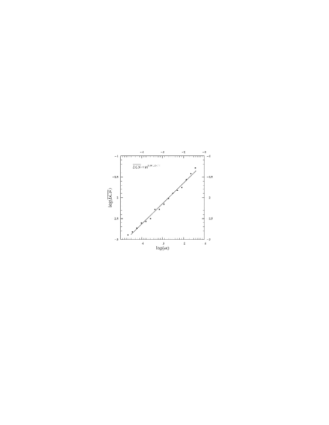
Figure 14: The $LCN\propto m^{1/2}$ relation in the case of the toy model potential (5). For each value of $\log(m)$ we have plotted the logarithm of the mean value of the Lyapunov exponents $\log(\overline{LCN})$ of an ensemble of orbits with random initial conditions in the phase space section corresponding to various energy levels.

References

- Allen et al. (1990) Allen A., Palmer P., Papaloizou J., 1990, MNRAS, 242, 576
- Contopoulos et al. (2002) Contopoulos G., Voglis N., Kalapotharakos C., 2002, Cel. Mech. Dyn. Astron., 83, 191
- Crane et al. (1993) Crane P., Stiavelli M., King I., Deharveng J., Albrecht R., Barbieri C., Blades J., Boksenberg A., Disney M., Jakobsen P., Kamperman T., Machetto F., Mackay C., Paresce F., Weigelt G., Baxter D., Greenfield P., Jedrzejewski R., Nota A., Sparks W., 1993, AJ, 106, 1371
- Cretton & van den Bosch (1999) Cretton N., van den Bosch F. C., 1999, ApJ, 514, 704
- de Zeeuw & Lynden-Bell (1985) de Zeeuw T., Lynden-Bell D., 1985, MNRAS, 215, 713
- Efthymiopoulos et al. (2007) Efthymiopoulos C., Voglis N., Kalapotharakos C., 2007, in Benest D., Froeschlé C., Lega E., eds, Topics in Gravitational Dynamics Vol. 729 of Lecture Notes In Physics. Springer, Berlin, p. 295
- Faber et al. (1997) Faber S. M., Tremaine S., Ajhar E. A., Byun Y., Dressler A., Gebhardt K., Grillmair C., Kormendy J., Lauer T. R., Richstone D., 1997, AJ, 114, 1771
- Ferrarese et al. (1994) Ferrarese L., van den Bosch F., Ford H., Jaffe W., O’Connell R., 1994, AJ, 108, 1598
- Fridman & Merritt (1997) Fridman T., Merritt D., 1997, AJ, 114, 1479
- Gebhardt et al. (1996) Gebhardt K., Richstone D., Ajhar E. A., Lauer T. R., Byun Y., Kormendy J., Dressler A., Faber S. M., Grillmair C., Tremaine S., 1996, AJ, 112, 105
- Gebhardt et al. (2000) Gebhardt K., Richstone D., Kormendy J., Lauer T. R., Ajhar E. A., Bender R., Dressler A., Faber S. M., Grillmair C., Magorrian J., Tremaine S., 2000, AJ, 119, 1157
- Gerhard & Binney (1985) Gerhard O. E., Binney J., 1985, MNRAS, 216, 467
- Holley-Bockelmann et al. (2001) Holley-Bockelmann K., Mihos J. C., Sigurdsson S., Hernquist L., 2001, ApJ, 549, 862
- Holley-Bockelmann et al. (2002) Holley-Bockelmann K., Mihos J. C., Sigurdsson S., Hernquist L., Norman C., 2002, ApJ, 567, 817
- Jesseit et al. (2005) Jesseit R., Naab T., Burkert A., 2005, MNRAS, 360, 1185
- Kalapotharakos & Voglis (2005) Kalapotharakos C., Voglis N., 2005, Cel. Mech. Dyn. Astron., 92, 157