BIASED RANGE TREES

Abstract

A data structure, called a biased range tree, is presented that preprocesses a set $S$ of $n$ points in $\mathbb{R}^{2}$ and a query distribution $D$ for 2-sided orthogonal range counting queries. The expected query time for this data structure, when queries are drawn according to $D$, matches, to within a constant factor, that of the optimal decision tree for $S$ and $D$. The memory and preprocessing requirements of the data structure are $O(n\log n)$.

1 Introduction

Let $S$ be a set of $n$ points in $\mathbb{R}^{2}$ and let $D$ be a probability measure over $\mathbb{R}^{2}$. A 2-sided orthogonal range counting query over $S$ asks, for a query point $q=(q_{x},q_{y})$, to report the number of points $(p_{x},p_{y})\in S$ such that $p_{x}\geq q_{x}$ and $p_{y}\geq q_{y}$. A 2-sided range counting query has distribution $D$ if the query point $q$ is chosen from the probability measure $D$. If $T$ is a data structure for answering 2-sided range counting queries over $S$ then we denote by $\mu_{D}(T)$ the expected time, using $T$, to answer a range query with distribution $D$. The current paper is concerned with preprocessing the pair $(S,D)$ to build a data structure $T$ that minimizes $\mu_{D}(T)$.

1.1 Previous Work

The general topic of geometric range queries is a field that has seen an enormous amount of activity in the last century. Results in this field depend heavily on the types of objects the data structure stores and on the shape of the query ranges. In this section we only mention a few data structures for orthogonal range counting and semigroup queries in 2 dimensions. The interested reader is directed to the excellent, and easily accessible, survey by Agarwal and Erickson [9].

Orthogonal range counting is a classic problem in computational geometry. The 2- (and 3- and 4-) sided range counting problem can be solved by Bentley’s range trees [3]. Range trees use $O(n\log n)$ space and can be constructed in $O(n\log n)$ time. Originally, range trees answered queries in $O(\log^{2}n)$ time. However, with the application of fractional cascading [6, 11] the query time can be reduced to $O(\log n)$ without increasing the space requirement by more than a constant factor. Range trees can also answer more general semigroup queries in which each point of $S$ is assigned a weight from a commutative semigroup and the goal is to report the weight of all points in the query range [10, 15].

For 2-sided orthogonal range counting queries, Chazelle [4, 5] proposes a data structure of size $O(n)$, that can be constructed in $O(n\log n)$ time, and that can answer range couting queries in $O(\log n)$ time. Unfortunately, this data structure is not capable of answering semigroup queries in the same time bound. For semigroup queries, Chazelle provides data structures with the following requirements: (1) $O(n)$ space and $O(\log^{2+\epsilon}n)$ query time, (2) $O(n\log\log n)$ space and $O(\log^{2}n\log\log n)$ query time, and (3) $O(n\log^{\epsilon}n)$ space and $O(\log^{2}n)$ query time.

Practical linear space data structures for range counting include $k$-d trees [2], quad-trees [13], and their variants. These structures are practical in the sense that they are easy to implement and use only $O(n)$ space. Unfortunately, neither of these structures has a worst-case query time of $\log^{O(1)}n$. Thus, in terms of query time, $k$-d trees and quad-trees are nowhere near competitive with range trees.

Despite the long history of data structures for orthogonal range queries, range trees with fractional cascading are still the most effective data structure for 2-sided orthogonal range queries in the semigroup model. In particular, no data structure is currently known that uses $o(n\log n)$ space and can answer 2-sided orthogonal range queries in $O(\log n)$ time.

1.2 New Results

In the current paper we present a data structure, the biased range tree, for 2-sided orthogonal range counting. Biased range trees fit into the comparison tree model of computation, in which all decisions made during a query are based on the result of comparing either the $x$- or $y$-coordinate of the query point to some precomputed values. Most data structures for orthogonal range searching, including range trees, $k$-d trees and quadtrees, fit into the comparison tree model. This model makes no assumptions about the $x$- or $y$-coordinates of points other than that they each come from some (possibly different) total order. This is particularly useful in practice since it avoid the precision problems usually associated with algebraic decisions and allows the mixing of different data types (one for $x$-coordinates and one for $y$-coordinates) in one data structure.

A biased range tree has size $O(n\log n)$, can be constructed in $O(n\log n)$ time, and can answer range counting (or semigroup) queries in $O(\mu_{D}(T^{*}))$ expected time, where $T^{*}$ is any comparison tree that answers range counting queries over $S$. In particular, $T^{*}$ could be a comparison tree that minimizes $\mu_{D}(T^{*})$ implying that the expected query time of our data structure is as fast as the fastest comparison-based data structure for answering range counting queries over $S$. Moreover, the worst-case search time of biased range trees is $O(\log n)$, matching the worst-case performance of range trees.

Note that we do not place any restrictions on the comparison tree $T^{*}$. Biased range trees, while requiring only $O(n\log n)$ space, are competitive with any comparison-based data structure. Thus, the memory requirement of biased range trees is the same as that of range trees but their expected query time can never be any worse.

The remainder of the paper is organized as follows. In Section 2 we present background material that is used in subsequent sections. In Section 3 we define biased range trees. In Section 4 we prove that biased range trees are optimal. In Section 5 we recap, summarize, and describe directions for future work.

2 Preliminaries

In this section we give definitions, notations, and background that are prerequisites for subsequent sections.

Rectangles.

For the purposes of the current paper, a rectangle $R(a,b,c,d)$ is defined as

$$R(a,b,c,d)=\{(x,y):\mbox{$a\leq x\leq b$ and $c\leq y\leq d$}\}\enspace.$$

We also allow unbounded rectangles by setting $a,c=-\infty$ and/or $b,d=\infty$. Therefore, under this definition, rectangles can have 0, 1, 2, 3, or 4 sides. For a query point $q=(q_{x},q_{y})$ we denote by $R(q)$ the query range $R(q_{x},\infty,q_{y},\infty)$. A horizontal strip is rectangle of the form $R(-\infty,\infty,c,d)$ and a vertical strip is a rectangle of the form $R(a,b,-\infty,\infty)$.

Classification Problems and Classification Trees.

A classification problem over a domain $\mathcal{D}$ is a function $\mathcal{P}:\mathcal{D}\mapsto\{0,\ldots,k-1\}$. The special case in which $k=2$ is called a decision problem. A $d$-ary classification tree is a full $d$-ary tree in which each internal node $v$ is labelled with a function $P_{v}:\mathcal{D}\mapsto\{0,.\ldots,d-1\}$ and for which each leaf $\ell$ is labelled with a value in $\{0,\ldots,k-1\}$. The search path of an input $q$ in a classification tree $T$ starts at the root of $T$ and, at each internal node $v$, evaluates $i=P_{v}(q)$ and proceeds to the $i$th child of $v$. We denote by $T(q)$ the label of the final (leaf) node in the search path for $q$. We say that the classification tree $T$ solves the classification problem $\mathcal{P}$ over the domain $\mathcal{D}$ if, for every $q\in\mathcal{D}$, $\mathcal{P}(q)=T(q)$.

The particular type of classification trees we are concerned with are comparison trees. These are binary classification trees in which the function $P_{v}$ at each node $v$ compares either $q_{x}$ or $q_{y}$ to a fixed value (that may depend on the point set $S$ and the distribution $D$). For the problem of 2-sided range counting over $S$, the leaves of $T$ are labelled with values in $\{0,\ldots,|S|\}$ and $T(q)=|R(q)\cap S|$ for all $q\in\mathbb{R}^{2}$.

Probability.

For a probability measure $D$ and an event $X$, we denote by $D_{|X}$ the distribution $D$ conditioned on $X$. That is, the distribution where the probability of an event $Y$ is $\Pr(Y\mid X)=\Pr(Y\cap X)/\Pr(X)$. The probability measures used in this paper are usually defined over $\mathbb{R}^{2}$. We make no assumptions about how these measures are represented, but we assume that an algorithm can, in constant time, given a rectangle $r$, determine $\Pr(r)$.

For a classification tree $T$ that solves a problem $P:\mathcal{D}\mapsto\{0,\ldots,k-1\}$ and a probability measure $D$ over $\mathcal{D}$, the expected search time of $T$, denoted by $\mu_{D}(T)$, is the expected length of the search path for $q$ when $q$ is drawn at random from $\mathcal{D}$ according to $D$. Note that, for each leaf $\ell$ of $T$ there is a maximal subset $r(\ell)\subseteq\mathcal{D}$ such that the search path for any $q\in r(\ell)$ ends at $\ell$. Thus, the expected search time of $T$ (under distribution $D$) can be written as

$$\mu_{D}(T)=\sum_{\ell\in L(T)}\Pr(r(\ell))\times 0pt_{T}(\ell)\enspace,$$

where $L(T)$ denotes the leaves of $T$ and $0pt_{T}(\ell)$ denotes the length of the path from the root of $T$ to $\ell$. When the tree $T$ is obvious based on context we will sometimes use the notation $d(\ell)$ to denote $d_{T}(\ell)$. Note that, for comparison trees, the closure of $r(\ell)$ is always a rectangle. For a node $v$ in a tree, we will use the phrases depth of $v$ and level of $v$ interchangeably and they both refer to $d(v)$.

The following theorem is a restatement of (half of) Shannon’s Fundamental Theorem for a Noiseless Channel [14, Theorem 9].

Theorem 1.

Let $\mathcal{P}:\mathcal{D}\mapsto\{0,\ldots,k-1\}$ be a classification problem and let $p\in\mathcal{D}$ be selected from a distibution $D$ such that $\Pr\{\mathcal{P}(p)=i\}=p_{i}$, for $0\leq i<k$. Then, any $d$-ary classification tree $T$ that solves $\mathcal{P}$ has

$$\mu_{D}(T)\geq\sum_{i=0}^{k-1}p_{i}\log_{d}(1/p_{i})\enspace.$$ (1)

In terms of range counting, Theorem 1 immediately implies that, if $p_{i}$ is the probability that the query range contains $i$ points of $S$, then any binary decision tree $T$ that does range counting has $\mu_{D}(T)\geq\sum_{i=0}^{n}p_{i}\log(1/p_{i})$. Unfortunately for us, this lower bound is too weak and, in general, there is no decision tree whose performance matches this obvious entropy lower bound.

A stronger lower bound on the cost of range searching can be obtained by considering the arrangement $A$ of $2n$ rays obtained by drawing two rays originating at each point of $S$, one to the left and one downwards (see Figure 1.a). This arrangement partitions the plane into a set of faces $F(A)$. If $T$ is a comparison tree for range counting in $S$, then there is no leaf $\ell$ of $T$ such that the interior of $r(\ell)$ intersects any edge of $A$ since otherwise there are query points $q$ in the neighbourhood of this intersection for which $T(q)\neq|R(q)\cap S|$. Therefore, by relabelling the leaves of $T$ with the faces of $A$, we obtain a data structure for determining which face of $A$ contains the query point $q$. By Theorem 1, this implies that

$$\mu_{D}(T)\geq\sum_{f\in F(A)}\Pr(f)\log(1/\Pr(f))\enspace.$$

Unfortunately, this bound is still not strong enough and, in general, there is no decision tree $T$ that matches this lower bound. To see this, consider Figure 1.b, when the query point $q$ is uniformly distributed among the $n+1$ shaded circles. In this case, $q$ is always in the same face of $A$ so the lower bound given above is 0. Nevertheless, it is not hard to see that the leaves of any decision tree $T$ for range searching in $S$ can be relabelled to determine which of the $n+1$ circles contains $q$, so $\mu_{D}(T)\geq\log(n+1)$.

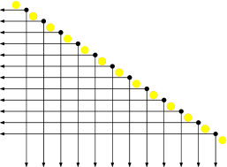
(a)	(b)

Figure 1: (a) The distribution of the query point $q$ over the faces of the arrangement $A$ gives a lower bound on the cost of any comparison tree for range counting in $S$. (b) The lower bound is not always achievable by a comparison tree.

Biased Search Trees.

Biased search trees are a classic data structure for solving the following 1-dimensional problem: Given an increasing sequence of real numbers $X=\langle x_{0}=-\infty,x_{1},x_{2},\ldots,x_{n},x_{n+1}=\infty\rangle$ and a probability distribution $D$ over $\mathbb{R}$, construct a binary search tree $T=T(X,D)$ so that, for any query value $q$ drawn from $D$, one can quickly find the unique interval $[x_{i},x_{i+1})$ containing $q$. If $p_{i}$ is the probability that $q\in[x_{i},x_{i+1})$ then the expected number of comparisons performed while searching for $q$ is given by

$$\mu_{D}(T)\leq\sum_{i=1}^{n}p_{i}\log(1/p_{i})+1$$

and the tree $T$ can be constructed in $O(n)$ time [12]. Clearly, by Theorem 1, the query time of this binary search tree is optimal up to an additive constant term. Note that, by having each node of $T$ store the size of its subtree, a biased search tree can count the number of elements of $X$ in the interval $I(q)=[q,\infty)$ without increasing the search time by more than a constant factor. Thus, biased search trees are an optimal data structure for 1-dimensional range counting.

3 Biased Range Trees

In this section we describe the biased range tree data structure, which has three main parts: the backup tree, the primary tree, and a set of catalogues that adorn the nodes of the primary tree.

3.1 The Backup Tree

In trying to achieve optimal query time, biased range trees will try to quickly answer queries that are, in some sense, easy. In some cases, a query is difficult and it cannot be answered in $o(\log n)$ time. For these queries, a backup range tree that stores the points of $S$ and can answer any 2-sided range query in $O(\log n)$ worst-case time is used. The preprocessing time and space requirements of this backup tree are $O(n\log n)$ [8].

3.2 The Primary Tree

Like a range tree, a biased range tree is an augmented data structure consisting of a primary tree whose nodes store secondary structures. However, in a range tree the primary tree is a binary search tree that discriminates based only on the $x$-coordinate of the query point $q$. In order to achieve optimal expected query time, this turns out to be insufficient, so instead biased range trees use a variation of a $k$-d tree as the primary tree.

The primary tree is constructed in a top-down fashion. Each node $v$ of $T$ is associated with a region $r(v)$ whose closure is a rectangle. The region associated with the root of $T$ is all of $\mathbb{R}^{2}$. We say that a node $v$ is bad if its depth is at least $\left\lceil\log_{2}n\right\rceil$ and $r(v)\cap S\neq\emptyset$. A node $v$ is split if $v$ its depth is less than $\left\lceil\log_{2}n\right\rceil$, and $r(v)\cap S\neq\emptyset$. The two children of a split node $v$ are associated with the two regions obtained by removing a horizontal or vertical strip $s(v)$ from $r(v)$ depending on whether the depth of $v$ is even or odd, respectively. We call a node $v$ at even distance from the root a vertical node, otherwise we call $v$ a horizontal node.

Refer to Figure 2. For a vertical node $v$, we denote its children by $\operatorname{left}(v)$ and $\operatorname{right}(v)$ and call them the left child and right child of $v$, depending on which side of the vertical strip (left or right) they are. For uniformity, we will also call the children of a node $v$ that is split with a horizontal strip $\operatorname{left}(v)$ and $\operatorname{right}(v)$. The child below the strip is denote by $\operatorname{left}(v)$ and the child above the strip is denoted by $\operatorname{right}(v)$. Similarly, the left and right boundaries of a strip $s(v)$ at a horizontal node $v$ refer to the bottom and top sides of $s(v)$. Note that, with these conventions, if the query point $q$ is in $r(\operatorname{left}(v))$ then $R(q)$ intersects $r(\operatorname{right}(v))$. However, if $q\in r(\operatorname{right}(v))$ then $R(q)$ does not intersect $r(\operatorname{left}(v))$. Similarly, for a query point $q\in s(v)$, the query range $R(q)$ intersects $r(\operatorname{right}(v))$ but not $r(\operatorname{left}(v))$

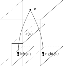
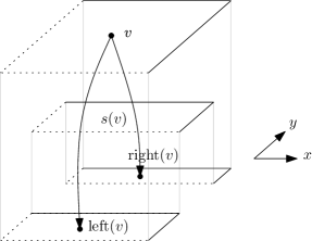
(a)	(b)

Figure 2: The splitting of (a) a vertical node $v$ and (b) a horizontal node $v$.

All that remains is to define the strip $s(v)$ for each node $v$. If $v$ is a leaf then we use the convention that $s(v)=r(v)$. If $v$ is not a leaf then $s(v)\subseteq r(v)$ is selected as a maximal strip containing no point of $r(v)\cap S$ in its interior, that is closed on its right side and open on its left side and such that each of the at most two components of $r(v)\setminus s(v)$ has probability at most $\Pr(r(v))/2$. Suppose $v$ is a vertical node. Then let $r(v)_{1},\ldots,r(v)_{k}$, be a partitioning of $r(v)$ into strips, in left-to-right order, obtained by drawing a vertical line through each of the $k$ points in $S\cap r(v)$. We use the convention that each strip is closed on its right side and open on its left side. Then there is a unique strip $s(v)=r(v)_{i}$ such that $\sum_{j=1}^{i-1}\Pr(r(v)_{j})\leq\Pr(r(v))/2$ and $\sum_{j=i+1}^{k}\Pr(r(v)_{j})<\Pr(r(v))/2$. For a horizontal node $v$, the definition of $s(v)$ is analagous except we use horizontal lines through each point of $r(v)\cap S$.

Note that for a node $v$ that is not a leaf, we use the convention that $s(v)$ contains its right side but not its left side and that $r(\operatorname{right}(v)$ and $r(\operatorname{left}(v))$ are the two components of $r(v)\setminus s(v)$. This implies that $r(\operatorname{left}(v))$ and/or $r(\operatorname{right}(v))$ may be empty, in which case $\operatorname{left}(v)$, respectively, $\operatorname{right}(v)$ is a leaf of $T$. With these definitions, for any point $q\in\mathbb{R}^{2}$ there is exactly one vertex $v$ of $T$ such that $q\in s(v)$.

The following two properties are easily derived from the definition of $T$ and are necessary to prove the optimality of biased range trees:

1. Any node $v$ at depth $i$ in $T$ has $\Pr(s(v))\leq\Pr(r(v))\leq 1/2^{i}$.

2. For any node $v$ of $T$, if $\Pr(r(v))>0$, then the closure of $r(v)$ contains at least one point of $S$.

Point 1 above follows immediately from the definition of $s(v)$. Next we explain the logic leading to Point 2. If $r(v)$ contains a point of $S$ then so does the closure of $r(v)$. If $r(v)=\emptyset$, then $\Pr(r(v))=0$. Otherwise, $r(v)\neq\emptyset$ and $r(v)$ has no point of $S$ in its interior. Then consider the parent $w$ of $v$. Since $s(w)$ does not contain $r(v)$ there must be a point of $S$ on the boundary of $s(w)$ that is also on the boundary of $r(v)$. Therefore $r(v)$ contains this point in its closure.

3.3 The Catalogues

The nodes of the tree $T$ are augmented with additional data structures called catalogues that hold subsets of $S$. Each node $v$ has two catalogues, $C_{x}(v)$ and $C_{y}(v)$ that store subsets of $S$ sorted by their $x$-, respectively, $y$-, coordinate. Intuitively, $C_{x}(v)$ stores points that are “above” $r(v)$ and $C_{y}(v)$ stores points that are “to the right of” $r(v)$. (Refer to Figure 3.) More precisely, if $v$ is a horizontal node, then $C_{x}(\operatorname{left}(v))=(s(v)\cup r(\operatorname{right}(v)))\cap S$ and $C_{y}(\operatorname{left}(v))=\emptyset$. If $v$ is a vertical node, then $C_{y}(\operatorname{left}(v))=(s(v)\cup r(\operatorname{right}(v)))\cap S$ and $C_{x}(\operatorname{left}(v))=\emptyset$. For any node $v$ that is the root of $T$ or a right child of its parent, $C_{x}(v)=C_{y}(v)=\emptyset$.

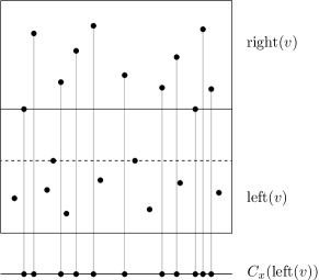
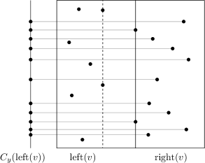
(a)	(b)

Figure 3: The catalogues of (a) a horizontal node $v$ and (b) a vertical node $v$.

Consider any node $v$ that is not a bad leaf and any point $q\in s(v)$. If $v$ has a left child then let $v_{1}=\operatorname{left}(v)$, otherwise, let $v_{1}=v$. Let $v_{1},\ldots,v_{k}$ denote the path from $v_{1}$ to the root of $T$ (see Figure 4). Then the catalogues of $v_{1},\ldots,v_{k}$ have the following properties:

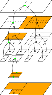
Figure 4: The area covered by catalogues on the path $v$ to the root of $T$. The $\times$ symbol shows the location of the query point $q$.

1. The points in the catalogues of $v_{1},\ldots,v_{k}$ are above or to the right of $q$. That is, for each $1\leq i\leq k$, all points in $C_{y}(v_{i})$, respectively, $C_{x}(v_{i})$ have their $x$-, respectively, $y$-, coordinate greater than or equal to $q_{x}$, respectively, $q_{y}$.

2. All catalogues at nodes in $v_{1},\ldots,v_{k}$ are disjoint. That, is, for each $1\leq i\leq j\leq k$, $C_{x}(v_{i})\cap C_{x}(v_{j})=\emptyset$, $C_{y}(v_{i})\cap C_{y}(v_{j})=\emptyset$, $C_{x}(v_{i})\cap C_{y}(v_{j})=\emptyset$, and $C_{x}(v_{j})\cap C_{y}(v_{i})=\emptyset$.

3. The catalogues at nodes $v_{1},\ldots,v_{k}$ contain all points in the query range $R(q)$. That is,

   $$R(q)\cap S\subseteq\bigcup_{i=1}^{k}\left(C_{x}(v_{i})\cup C_{y}(v_{i})\right)\enspace.$$

Note that, points 1, 2 and 3 above imply that determining $|R(q)\cap S|$ can be done by solving a sequence of 1-sided range queries in the $x$- and $y$-catalogues of $v_{1},\ldots,v_{k}$. However, performing these queries individually would take too long.

To speed up the process of navigating the catalogues of $T$, fractional cascading [6] is used. Starting at the root of $T$ and as long as $v$ is not a leaf, a fraction of the data in $C_{x}(v)$ is cascaded into $C_{x}(\operatorname{right}(v))$ and $C_{x}(\operatorname{left}(v))$. As well, a fraction of the data in $C_{y}(v)$ is cascaded into both $C_{y}(\operatorname{right}(v))$ and $C_{y}(\operatorname{left}(v))$. Note that this cascading is done only to speed up navigation between the catalogues of $T$. Although fractional cascading introduces extra data into the catalogues of $T$ we will continue to use the notations $C_{x}(v)$ and $C_{y}(v)$ to denote the set of points contained in the catalogues of $v$ before fractional cascading takes place.

Finally, each catalogue $C_{x}(v)$ and $C_{y}(v)$ is indexed by a biased binary search tree $T_{x}(v)$, respectively, $T_{y}(v)$. If $v$ is the left child of its parent, then the weight of an interval $(a,b]$ in $T_{x}(v)$, respectively, $T_{y}(v)$ is given by the probability that $q_{x}$, respectively, $q_{y}$, is in the interval $(a,b]$ when $q$ is drawn according to the distribution $D_{\mid s(\operatorname{parent}(v))}$. Otherwise ($v$ is not a left child), the weight of an interval is determined by the distribution $D_{\mid s(v)}$.

3.4 Construction Time and Space Requirements

The biased range tree data structure is now completely defined. The structure consists of a backup tree, a primary tree, and the catalogues of the primary tree. We now analyze the construction time and space requirements of biased range trees.

The backup tree has size $O(n\log n)$ and can be constructed in $O(n\log n)$ time [8, Theorem 5.11]. To construct the primary tree quickly we presort the points of $S$ by their $x$ and $y$ coordinates. Since the primary tree has height $O(\log n)$, it is then easily constructed in $O(n\log n)$ time. Ignoring any copies of points created by fractional cascading, each point in $S$ occurs in at most 2 catalogues at each level of the primary tree. Thus, the sizes of all catalogues (before fractional cascading) is $O(n\log n)$ and these catalogues can be constructed in $O(n\log n)$ time (because of elements of $S$ are presorted; see de Berg et al. [8, Section 5.3] for details). The fractional cascading between catalogues does not increase the size of catalogues by more than a constant factor since each catalogue is cascaded into only a constant number of other catalogues [6].

In summary, given the point set $S$ and access to the distribution $D$, a biased range tree for $(S,D)$ can be constructed in $O(n\log n)$ time and requires $O(n\log n)$ space.

3.5 The Query Algorithm

The algorithm to answer a 2-sided range query $q=(q_{x},q_{y})$ proceeds in three steps:

1. The algorithm navigates the tree $T$ from top to bottom to locate the unique node $v$ such that $q\in s(v)$. This step takes $O(d_{T}(q))$ time, where $d_{T}(q)$ is the depth of the node $v$. If $v$ is a bad leaf (so $d_{T}(q)\geq\log n$) then the algorithm performs a range query in $O(\log n)$ time using the backup range tree and the query algorithm does not execute the next two steps.

2. If $v$ has a left child then let $u=\operatorname{left}(v)$, otherwise let $u=v$. The algorithm uses $T_{x}(u)$ and $T_{y}(u)$ to locate $q_{x}$ and $q_{y}$, respectively, in the catalogues $C_{x}(u)$ and $C_{y}(u)$, respectively.

3. The algorithm walks back from $u$ to the root of $T$, locating $q$ in the catalogues of all nodes on this path and computing the results of the range counting query as it goes. Thanks to fractional cascading, each step of this walk can be done in constant time, so the overall time for this step is also $O(d_{T}(q))$.

Observe that Steps 1 and 3 of the query algorithm each take $O(d_{T}(q))$ time. The time needed to accomplish Step 2 of the algorithm depends on exactly what is in the catalogues $C_{x}(u)$ and $C_{y}(u)$, and will be the first quantity we study in the next section.

4 Optimality of Biased Range Trees

In this section we show that the expected query time of biased range trees is as good as the expected query time of any comparison tree. The expected query time has two components. The first component is the expected depth, $d_{T}(q)$, of the node $v$ such that $s(v)$ contains $q$. The second component is the expected cost of locating $q$ in the catalogues of $u$ (recall that $u=\operatorname{left}(v)$ or $u=v$ if $v$ has no left child). We will show that each of these two components is a lower bound on the expected cost of any decision tree for two-sided range searching on $S$ where queries come from distribution $D$. In order to simplify notation in this section we will use the convention $\Pr(v)=\Pr(s(v))$ is the probability that a search terminates at node $v$ of $T$.

4.1 The Catalogue Location Step

First we show that the expected cost of locating $q$ in the two catalogues, $C_{x}(u)$ and $C_{y}(u)$ is a lower bound on the expected cost of any decision tree for answering 2-sided range queries in $S$. The intuition behind this proof is that, in order to correctly answer range counting queries, any decision tree for range counting must locate the $x$-coordinate of $q$ with respect to the $x$-coordinates of all points above $q$. Similarly, it must locate the $y$-coordinate of $q$ with respect to the $y$-coordinates of all points to the right of $q$. The structure of the catalogues ensures that biased range trees do this in the most efficient manner possible.

Lemma 1.

Let $S$ be a set of $n$ points and let $D$ be a probability measure over $\mathbb{R}^{2}$. Let $T^{*}$ be any decision tree for 2-sided range counting in $S$ and let $C_{2}(S,D)$ denote the expected cost of locating $q$ in Step 2 of the biased range tree query algorithm on the biased range tree $T=T(S,D)$. Then

$$\mu_{D}(T^{*})=\Omega(C_{2}(S,D))\enspace.$$

Proof.

We first observe that, by definition,

$$C_{2}(S,D)=\sum_{v\in T}\Pr(v)\left(\mu_{D_{\mid s(v)}}(T_{x}(u))+\mu_{D_{\mid s(v)}}(T_{y}(u))\right)\enspace.$$

Consider some node $v$ of $T$. For a point $q\in s(v)$, all of the points in $T_{x}(v)$ are points that may or may not be in the query range $R(q)$ depending on where exactly $q$ is located within $s(v)$. This implies that, if $T^{*}$ correctly answers range queries for every point $q\in s(v)$ then it must determine the location of the $x$-coordinate of $q$ with respect to all points in $T_{x}(v)$. More precisely, the leaves of $T^{*}$ could be relabelled to obtain a comparison tree that determines, for any $q\in s(v)$, which interval of $T_{x}(v)$ contains $q_{x}$. Since $T_{x}(u)$ is a biased search tree for the probability measure $D_{\mid s(v)}$, this implies that

$$\mu_{D_{\mid s(v)}}(T^{*})\geq\mu_{D_{\mid s(v)}}(T_{x}(u))-1\enspace.$$

Similarly, the same argument applied to $T_{y}(v)$ yields

$$\mu_{D_{\mid s(v)}}(T^{*})\geq\mu_{D_{\mid s(v)}}(T_{y}(u))-1\enspace.$$

We can now complete the proof with

$$\mu_{D}(T^{*}) = \sum_{v\in T}\Pr(v)\cdot\mu_{D_{\mid s(v)}}(T^{*})$$

$$\geq \sum_{v\in T}\Pr(v)\cdot\max\left\{\mu_{D_{\mid s(v)}}(T_{x}(u)),\mu_{D_{\mid s(v)}}(T_{y}(u))\right\}-1$$

$$\geq \sum_{v\in T}\frac{1}{2}\Pr(v)\cdot\left(\mu_{D_{\mid s(v)}}(T_{x}(u))+\mu_{D_{\mid s(v)}}(T_{y}(u))\right)-1$$

$$= \frac{1}{2}\cdot C_{2}(S,D)-1=\Omega(C_{2}(S,D))\enspace.$$

∎

4.2 The Tree Searching Step

Next we bound the expected depth $d_{T}(q)$ of the node $v$ of $T$ such that $q\in s(v)$. We do this by showing that any decision tree $T^{*}$ for range counting in $S$ must solve a set of point location problems and that the expected depth of $v$ is a lower bound on the complexity of solving these problems.

We say that a set of rectangles is HV-independent if no horizontal or vertical line intersects more than one rectangle in the set. We say that a set $\{v_{1},\ldots,v_{k}\}$ of nodes in $T$ is HV-independent if the set $\{r(v_{1}),\ldots,r(v_{k})\}$ is HV-independent.

Lemma 2.

Let $S$ be a set of $n$ points and let $D$ be a probability measure over $\mathbb{R}^{2}$. Let $T=T(S,D)$ be the biased range tree for $(S,D)$ and label each node of $T$ white or black, such that all white nodes are at distance at most $i$ from the root of $T$. Then, if $T$ contains more than $\gamma^{i}$ white nodes then $T$ contains an HV-independent set of white nodes of size $\Omega((\gamma/\sqrt{2})^{i})$.

Proof.

Define a graph $G=(V,E)$ whose vertices are the white nodes of $T$ and for which $uv\in E$ if and only if there is a horizontal or vertical line that intersects both $r(u)$ and $r(v)$. Note that an independent set of vertices in $G$ is an HV-independent set of which nodes in $T$. Thus, it suffices to find a sufficiently large independent set in $G$

A well-know result on $k$-d trees states that, for a $k$-d tree of height $i$, any horizontal or vertical line intersects at most $2^{\left\lceil i/2\right\rceil}$ rectangles of the $k$-d tree [8, Lemma 5.4]. Therefore, since $T$ is a $k$-d tree, the number of edges in $G$ is at most $|V|\cdot 2^{\left\lceil i/2\right\rceil}$. This implies that $G$ has a vertex $v$ of degree at most $2^{\left\lceil i/2\right\rceil+1}$ and this is also true of any vertex-induced subgraph of $G$.

We can therefore obtain an independent set in $G$ by repeatedly selecting a vertex $v$ of degree $2^{\left\lceil i/2\right\rceil+1}$, adding $v$ to the independent set and deleting $v$ and its neighbours from $G$. Since, at each step we add one vertex to the independent set and delete at most $2^{\left\lceil i/2\right\rceil+1}+1$ vertices from $G$, this produces an independent of size $\Omega(|V|/2^{i/2})=\Omega((\gamma/\sqrt{2})^{i})$, as required. ∎

We can now provide the second piece of the lower bound.

Lemma 3.

Let $S$ be a set of $n$ points and let $D$ be a probability measure over $\mathbb{R}^{2}$. Let $T^{*}$ be any comparison tree that does range counting over $S$. Let $C_{1}(S,D)$ denote the expected depth of the node $v$ of the biased range tree $T=T(S,D)$ such that $q\in s(v)$. Then

$$\mu_{D}(T^{*})=\Omega(C_{1}(S,D))$$

Proof.

Partition the nodes of $T$ into groups $G_{1},G_{2},\ldots$ where $G_{i}$ contains all nodes $v$ such that $1/2^{i}\leq\Pr(v)\leq 1/2^{i-1}$. Observe that the nodes in group $G_{i}$ occur in the first $i$ levels of $T$. Select a constants $\gamma$ and $\beta$ with $\sqrt{2}<\gamma<\beta<2$ and define $\alpha=\gamma/\sqrt{2}$. By repeatedly applying Lemma 2, each group $G_{i}$ can be partitioned into groups $G_{i,1},\ldots,G_{i,t_{i}}$ where, for each $1\leq j<t_{i}$, $G_{i,j}$ is an HV-independent set with $|G_{i,j}|\geq\alpha^{i}$. Furthermore, $|G_{i,t_{i}}|\leq\gamma^{i}$. (Note that $G_{i,t_{i}}$ is not necessarily HV-independent.)

Consider some group $G_{i,j}$ for $1\leq j<t_{i}$. Let $\ell$ be a leaf of $T^{*}$ and observe that, because the nodes in $G_{i,j}$ are independent and each one contains at least one point of $S$ in its closure, there are at most 4 nodes $v$ in $G_{i,j}$ such that $r(\ell)$ intersects the closure of $r(v)$. (Otherwise $r(\ell)$ contains a point of $S$ in its interior and therefore $T^{*}$ does not solve the range counting problem for $S$.) Thus, by performing 2 additional comparisons, $T^{*}$ can be used to determine which node of $v\in G_{i,j}$ (if any) contains the query point $q$ in $s(v)$. However, $G_{i,j}$ contains $\Omega(\alpha^{i})$ nodes and the search path for $q$ terminates at each of these with probability between $1/2^{i}$ and $1/2^{i-1}$. Therefore, if we denote by $D_{i,j}$ the distribution $D$ conditioned on the search path for $q$ terminating in one of the nodes in $G_{i,j}$ then we have, by applying Theorem 1,

$$\mu_{D_{i,j}}(T^{*})+2 \geq \sum_{v\in G_{i,j}}\Pr(v\mid G_{i,j})\log(1/\Pr(v\mid G_{i,j})$$

$$\geq \sum_{v\in G_{i,j}}\Pr(v\mid G_{i,j})\log(\Omega(\alpha^{i}))$$

$$\geq \log(\Omega(\alpha^{i}))$$

$$= i\log\alpha-O(1)\enspace.$$

Putting this all together, we obtain

$$\mu_{D}(T^{*}) = \sum_{i=1}^{\infty}\sum_{j=1}^{t_{i}}\Pr(G_{i,j})\mu_{D_{i,j}}(T^{*})$$

$$\geq \sum_{i=1}^{\infty}\sum_{j=1}^{t_{i}-1}\Pr(G_{i,j})\mu_{D_{i,j}}(T^{*})$$

$$\geq \sum_{i=1}^{\infty}\sum_{j=1}^{t_{i}-1}\Pr(G_{i,j})(i\log\alpha-O(1))$$

$$\geq (\log\alpha)\cdot\sum_{i=1}^{\infty}\sum_{j=1}^{t_{i}-1}\sum_{v\in G_{i,j}}\Pr(v)\cdot 0pt(v)-O(1)$$

$$= (\log\alpha)\cdot\sum_{v\in T}\Pr(v)\cdot 0pt(v)-\sum_{i=1}^{\infty}\sum_{v\in G_{i,t_{i}}}\Pr(v)\cdot 0pt(v)-O(1)$$

$$\geq (\log\alpha)\cdot\sum_{v\in T}\Pr(v)\cdot 0pt(v)-\sum_{i=1}^{\infty}i\cdot\Pr(G_{i,t_{i}})-O(1)$$

$$\geq (\log\alpha)\cdot\sum_{v\in T}\Pr(v)\cdot 0pt(v)-\sum_{i=1}^{\left\lceil\log n\right\rceil}i\gamma^{i}/2^{i-1}-O(1)$$

$$\geq (\log\alpha)\cdot\sum_{v\in T}\Pr(v)\cdot 0pt(v)-O(1)$$

$$= \Omega(C_{1}(S,D))\enspace,$$

where the last inequality follows from the fact that $\gamma/2<1$. ∎

To get some idea of the constants involved in the proof of Lemma 3, we can select $\gamma=1.6$, so that $\alpha=1.6/\sqrt{2}\approx 1.13137085$ and $\log\alpha\approx 0.178071905$ and the $O(1)$ term is approximately 20. Thus, for this choice of parameters, the depth in $T$ is competitive with $T^{*}$ to within a factor of $1/0.178071905\approx 5.615$ and an additive constant of 20. Alternatively, selecting $\gamma=1.8$ gives a constant factor less than 3 and an additive term of approximately 90.

And now the main event:

Theorem 2.

Let $S$ be a set of $n$ points and let $D$ be a probability measure over $\mathbb{R}^{2}$. Let $T=T(S,D)$ be the biased range tree for $S$ and $D$ and let $T^{*}$ be any decision tree that answers range counting queries for $S$. Then

$$\mu_{D}(T^{*})=\Omega(\mu_{D}(T))\enspace.$$

Proof.

By the definition of $C_{1}$ and $C_{2}$, the expected cost of searching in $T$ is $\mu_{D}(T)=O(C_{1}(S,D)+C_{2}(S,D))$. On the other hand, by Lemma 3 and Lemma 1 $\mu_{D}(T^{*})=\Omega(\max\{C_{1}(S,D),C_{2}(S,D)\})=\Omega(C_{1}(S,D)+C_{2}(S,D))=\Omega(\mu_{D}(T))$. This completes the proof. ∎

5 Summary, Discussion, and Conclusions

We have presented biased range trees, an optimal data structure for 2-sided orthogonal range counting queries when the point set $S$ and query distribution $D$ is known in advance. The expected time required to answer queries with a biased range tree, when the queries are distributed according to $D$, is within a constant factor of any decision tree for answering range queries over $S$. Like standard range trees, biased range trees use $O(n\log n)$ space and can also answer semigroup queries [10, 15]. Although the analysis of biased range trees is complicated, their implementation is not much more complicated than that of standard range trees.

As a small optimization, the backup range tree data structure can be eliminated from biased range trees. Instead, once the probability of a node $v$ drops below $1/n$ the node can be split by ignoring the distribution $D$ and simply splitting the points of $r(v)\cap S$ into two sets of roughly equal size. This results in a tree of depth at most $2(\log n+1)$.

This work is just one of many possible results on distribution-sensitive range searching. Several open problems immediately arise.

Open Problem 1.

Are there efficient distribution-sensitive data structures for 3-sided and 4-sided orthogonal range counting queries?

Note that a 4-sided orthogonal range counting query can be reduced to 4 2-sided orthogonal range counting queries using the principle of inclusion-exclusion. Unfortunately, this reduction does not produce an optimal distribution-sensitive data structure. To see this, consider 4-sided queries consisting of unit squares whose bottom left corner is uniformly distributed in the shaded region of Figure 5. All such queries contain no points in the query region and all such queries can be answered in $O(1)$ time by simply checking that all four corners of the square are to the left of the point set. However, when we decompose these queries into a four 2-sided queries we obtain 2-sided queries that require $\Omega(\log n)$ time to be answered.

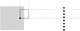
Figure 5: Decomposing a 4-sided query into four 2-sided queries can produce a bad distribution of 2-sided queries.

Open Problem 2.

Biased range trees require that the point set $S$ and the distribution $D$ be known in advance. Is there a self-adapting version of biased range trees that, without knowing $D$ in advance, can answer $m$ queries, each drawn independently from $D$ in $O(n\log n+m\mu_{D}(T^{*}))$ expected time?

Open Problem 3.

Determine the worst-case or the average case constants associated with 2-dimensional orthogonal range searching for comparison-based data structures. By applying the result of Adamy and Seidel [1] on point location to the arrangement $A$ described in Section 2 one immediately obtains an $O(n^{2})$ space data structure that answers queries using at most $2\log n+O(\log\log n)$ comparisons. Is there an $O(n\log n)$ space structure with the same performance?

Open Problem 4.

A point $q\in\mathbb{R}^{d}$ is maximal with respect to $S\subseteq\mathbb{R}^{d}$ if no point of $S$ has every coordinate larger than the corresponding coordinate of $q$. For $d\geq 3$, is there a distribution-sensitive data structure for testing if a query point $q$ is maximal? For point sets in 2 dimensions, an orthogonal variant of the point-location techniques of Collette et al. [7] seems to apply.

Open Problem 5.

Are there distribution-sensitive data structures for $d$-sided range search in point sets in $\mathbb{R}^{d}$? The current fastest structures for range search in point sets in $\mathbb{R}^{d}$ that use near-linear space have $\Theta(\log^{d-1}n)$ query time. Is there a structure that uses near-linear space and is optimal when the point set $S$ and the distribution $D$ are known in advance?

References

- [1] U. Adamy and R. Seidel. On the exact worst case query complexity of planar point location. In Proceedings of the Ninth Annual ACM-SIAM Symposium on Discrete Algorithms, pages 609–618, 1998.
- [2] J. L. Bentley. Multidimensional binary search trees used for associative searching. Communications of the ACM, 18:509–517, 1975.
- [3] J. L. Bentley. Multidimensional divide-and-conquer. Communications of the ACM, 23:214–229, 1980.
- [4] B. Chazelle. Filtering search: A new approach to query-answering. SIAM Journal on Computing, 15:703–724, 1986.
- [5] B. Chazelle. A functional approach to data structures and its use in multidimensional searching. SIAM Journal on Computing, 17:427–462, 1988.
- [6] B. Chazelle and L. J. Guibas. Fractional cascading: I. a data structuring technique. Algorithmica, 1:133–162, 1986.
- [7] S. Collette, V. Dujmović, J. Iacono, S. Langerman, and P. Morin. Distribution-sensitive point location in convex subdivisions. In Proceedings of the 19th ACM-SIAM Symposium on Discrete Algorithms (SODA 2008), 2008. Submitted to SIAM Journal on Computing, August 2007.
- [8] M. de Berg, M. van Kreveld, M. Overmars, and O. Schwarzkopf. Computational Geometry: Algorithms and Applications. Springer-Verlag, Heidelberg, 1997.
- [9] J. Erickson and P. K. Agarwal. Geometric range searching and its relatives. In B. Chazelle, J. E. Goodman, and R. Pollack, editors, Advances in Discrete and Computational Geometry, volume 223 of Contemporary Mathematics, pages 1–56. American Mathematical Society Press, 1999.
- [10] M. L. Fredman. A lower bound on the complexity of orthogonal range queries. Journal of the ACM, 28:696–705, 1981.
- [11] G. S. Luecker. A data structure for orthogonal range queries. In Proceedings of the 19th Annual IEEE Symposium on Foundations of Computer Science (FOCS), pages 28–34, 1978.
- [12] K. Mehlhorn. Nearly optimal binary search trees. Acta Informatica, 5:287–295, 1975.
- [13] H. Samet. The Design and Analysis of Spatial Data Structures. Addison-Wesley, Reading, MA, 1990.
- [14] C. E. Shannon. A mathematical theory of communication. Bell Systems Technical Journal, pages 379–423 and 623–656, 1948.
- [15] A. C. Yao. On the complexity of maintaining partial sums. SIAM Journal on Computing, 14:277–288, 1985.