”Magnetic” components of gravitational waves and response functions of interferometers

Abstract

Recently, arising from an enlighting analysis of Baskaran and Grishchuk in Class. Quant. Grav. 21 4041-4061 (2004), some papers in the literature have shown the presence and importance of the so-called “magnetic” components of gravitational waves (GWs), which have to be taken into account in the context of the total response functions of interferometers for GWs propagating from arbitrary directions. In Int. Journ. Mod. Phys. A 22, 13, 2361-2381 (2007) and Int. J. Mod. Phys. D 16, 9, 1497-1517 (2007) accurate response functions for the Virgo and LIGO interferometers have been analysed.

However, some results which have been shown in Int. Journ. Mod. Phys. A 22, 13, 2361-2381 (2007) look in contrast with the results which have been shown in Int. J. Mod. Phys. D 16, 9, 1497-1517 (2007). In fact, in Int. Journ. Mod. Phys. A 22, 13, 2361-2381 (2007) it was claimed that the “magnetic” component of GWs could, in principle, extend the frequency range of Earth based interferometers, while in Int. J. Mod. Phys. D 16, 9, 1497-1517 (2007) such a possibility has been banned.

This contrast has been partially solved in the Proceedings of the XLIInd Rencontres de Moriond, Gravitational Waves and Experimental Gravity, La Thuile, Val d’Aosta Italy (March 12-18 2007).

The aim of this review paper is to re-analyse all the framework of the “magnetic” components of GWs with the goal of solving the mentioned contrast in definitive way.

Accurate response funtions for the Virgo and LIGO interferometers will be also re-discussed in detail.

Associazione Scientifica Galileo Galilei, Via Pier Cironi 16 - 59100 PRATO, Italy; Dipartimento della Gravitazione, Centro Scienze Naturali, via di Galceti 74 - 59100 PRATO, Italy

E-mail address: christian.corda@ego-gw.it

PACS numbers: 04.80.Nn, 04.80.-y, 04.25.Nx

1 Introduction

The data analysis of interferometric gravitational waves (GWs) detectors has recently been started (for the current status of GWs interferometers see [1, 2, 3, 4, 5, 6, 7, 8]) and the scientific community aims in a first direct detection of GWs in next years.

Detectors for GWs will be important for a better knowledge of the Universe and also to confirm or ruling out the physical consistency of General Relativity or of any other theory of gravitation [9, 10, 11, 12, 13, 14, 15, 16]. This is because, in the context of Extended Theories of Gravity, some differences between General Relativity and the others theories can be pointed out starting by the linearized theory of gravity [9, 10, 12, 14]. In this picture, detectors for GWs are in principle sensitive also to a hypotetical scalar component of gravitational radiation, that appears in extended theories of gravity like scalar-tensor gravity, high order theories [12, 15, 16, 17, 18, 19, 20, 21, 22] and Brans-Dicke theory [23].

Recently, arising from an enlighting analysis of Baskaran and Grishchuk in [24], some papers in the literature have shown the presence and importance of the so-called “magnetic” components of GWs, which have to be taken into account in the context of the total response functions of interferometers for GWs propagating from arbitrary directions. In [25] and [26] accurate response functions for the Virgo and LIGO interferometers have been analysed.

However, some results which have been shown in [25] look in contrast with the results which have been shown in[26]. In fact, in [25] it was claimed that the “magnetic” component of GWs could, in principle, extend the frequency range of Earth based interferometers, while in [26] such a possibility has been banned.

This contrast has been partially solved in [27].

The aim of this review paper is to re-analyse all the framework of the “magnetic” components of GWs with the goal of solving the mentioned contrast in definitive way.

Accurate response funtions for the Virgo and LIGO interferometers will be re-discussed in detail too.

2 Analysis in the frame of the local observer

In a laboratory enviroment on earth, the coordinate system in which the space-time is locally flat is typically used and the distance between any two points is given simply by the difference in their coordinates in the sense of Newtonian physics [9, 12, 24, 25, 26, 27, 28]. In this frame, called the frame of the local observer, GWs manifest themself by exerting tidal forces on the masses (the mirror and the beam-splitter in the case of an interferometer, see figure 1).

Figure 1: photons can be launched from the beam-splitter to be bounced back by the mirror

Recently, the presence and importance of the so-called magnetic components of GWs have been shown by Baskaran and Grishchuk that computed the correspondent detector patterns in the low-frequencies approximation [24]. Then, more detailed angular and frequency dependences of the response functions for the magnetic components has been given in the same approximation, with a specific application to the parameters of the LIGO and Virgo interferometers in [25, 26, 27]. The most important goal of this review paper is to solve in a definitive way the contrast between [25] and [26] on the possibility of extending the frequency-band of interferometers.

Before starting with the analysis of the response functions, a brief review of Section 3 of [24] is due to understand the importance of the “magnetic” components of GWs. In this review paper we will use different notations with respect to the ones used in [24]. Following [25, 26, 27], we work with $G=1$, $c=1$ and $\hbar=1$ and we call $h_{+}(t_{tt}+z_{tt})$ and $h_{\times}(t_{tt}+z_{tt})$ the weak perturbations due to the $+$ and the $\times$ polarizations which are expressed in terms of synchronous coordinates $t_{tt},x_{tt},y_{tt},z_{tt}$ in the transverse-traceless (TT) gauge. In this way, the most general GW propagating in the $z_{tt}$ direction can be written in terms of plane monochromatic waves [25, 26, 27]

$$\begin{array}[]{c}h_{\mu\nu}(t_{tt}+z_{tt})=h_{+}(t_{tt}+z_{tt})e_{\mu\nu}^{(+)}+h_{\times}(t_{tt}+z_{tt})e_{\mu\nu}^{(\times)}=\\ \\ =h_{+0}\exp i\omega(t_{tt}+z_{tt})e_{\mu\nu}^{(+)}+h_{\times 0}\exp i\omega(t_{tt}+z_{tt})e_{\mu\nu}^{(\times)},\end{array}$$ (1)

and the correspondent line element will be

$$ds^{2}=dt_{tt}^{2}-dz_{tt}^{2}-(1+h_{+})dx_{tt}^{2}-(1-h_{+})dy_{tt}^{2}-2h_{\times}dx_{tt}dx_{tt}.$$ (2)

The wordlines $x_{tt},y_{tt},z_{tt}=const.$ are timelike geodesics representing the histories of free test masses [24, 25, 26, 27]. The coordinate transformation $x^{\alpha}=x^{\alpha}(x_{tt}^{\beta})$ from the TT coordinates to the frame of the local observer is [24, 25, 26, 27].

$$\begin{array}[]{c}t=t_{tt}+\frac{1}{4}(x_{tt}^{2}-y_{tt}^{2})\dot{h}_{+}-\frac{1}{2}x_{tt}y_{tt}\dot{h}_{\times}\\ \\ x=x_{tt}+\frac{1}{2}x_{tt}h_{+}-\frac{1}{2}y_{tt}h_{\times}+\frac{1}{2}x_{tt}z_{tt}\dot{h}_{+}-\frac{1}{2}y_{tt}z_{tt}\dot{h}_{\times}\\ \\ y=y_{tt}+\frac{1}{2}y_{tt}h_{+}-\frac{1}{2}x_{tt}h_{\times}+\frac{1}{2}y_{tt}z_{tt}\dot{h}_{+}-\frac{1}{2}x_{tt}z_{tt}\dot{h}_{\times}\\ \\ z=z_{tt}-\frac{1}{4}(x_{tt}^{2}-y_{tt}^{2})\dot{h}_{+}+\frac{1}{2}x_{tt}y_{tt}\dot{h}_{\times},\end{array}$$ (3)

where it is $\dot{h}_{+}\equiv\frac{\partial h_{+}}{\partial t}$ and $\dot{h}_{\times}\equiv\frac{\partial h_{\times}}{\partial t}$. The coefficients of this transformation (components of the metric and its first time derivative) are taken along the central wordline of the local observer [24, 25, 26, 27]. It is well known from [24, 25, 26, 27] that the linear and quadratic terms, as powers of $x_{tt}^{\alpha}$, are unambiguously determined by the conditions of the frame of the local observer, while the cubic and higher-order corrections are not determined by these conditions. Thus, at high-frequencies, the expansion in terms of higher-order corrections breaks down [24, 26, 27].

Considering a free mass riding on a timelike geodesic ($x=l_{1}$, $y=l_{2},$ $z=l_{3}$) [24, 25, 26, 27], eqs. (3) define the motion of this mass with respect to the introduced frame of the local observer. In concrete terms one gets

$$\begin{array}[]{c}x(t)=l_{1}+\frac{1}{2}[l_{1}h_{+}(t)-l_{2}h_{\times}(t)]+\frac{1}{2}l_{1}l_{3}\dot{h}_{+}(t)+\frac{1}{2}l_{2}l_{3}\dot{h}_{\times}(t)\\ \\ y(t)=l_{2}-\frac{1}{2}[l_{2}h_{+}(t)+l_{1}h_{\times}(t)]-\frac{1}{2}l_{2}l_{3}\dot{h}_{+}(t)+\frac{1}{2}l_{1}l_{3}\dot{h}_{\times}(t)\\ \\ z(t)=l_{3}-\frac{1}{4[}(l_{1}^{2}-l_{2}^{2})\dot{h}_{+}(t)+2l_{1}l_{2}\dot{h}_{\times}(t),\end{array}$$ (4)

which are exactly eqs. (13) of [24] rewritten using our notation. In absence of GWs the position of the mass is $(l_{1},l_{2},l_{3}).$ The effect of the GW is to drive the mass to have oscillations. Thus, in general, from eqs. (4) all three components of motion are present [24, 25, 26, 27].

Neglecting the terms with $\dot{h}_{+}$ and $\dot{h}_{\times}$ in eqs. (4), the “traditional” equations for the mass motion are obtained [24, 25, 26, 27]:

$$\begin{array}[]{c}x(t)=l_{1}+\frac{1}{2}[l_{1}h_{+}(t)-l_{2}h_{\times}(t)]\\ \\ y(t)=l_{2}-\frac{1}{2}[l_{2}h_{+}(t)+l_{1}h_{\times}(t)]\\ \\ z(t)=l_{3}.\end{array}$$ (5)

Clearly, this is the analogous of the electric component of motion in electrodynamics [24, 25, 26, 27], while equations

$$\begin{array}[]{c}x(t)=l_{1}+\frac{1}{2}l_{1}l_{3}\dot{h}_{+}(t)+\frac{1}{2}l_{2}l_{3}\dot{h}_{\times}(t)\\ \\ y(t)=l_{2}-\frac{1}{2}l_{2}l_{3}\dot{h}_{+}(t)+\frac{1}{2}l_{1}l_{3}\dot{h}_{\times}(t)\\ \\ z(t)=l_{3}-\frac{1}{4[}(l_{1}^{2}-l_{2}^{2})\dot{h}_{+}(t)+2l_{1}l_{2}\dot{h}_{\times}(t),\end{array}$$ (6)

are the analogous of the magnetic component of motion. One could think that the presence of these magnetic components is a “frame artefact” due to the transformation (3), but in Section 4 of [24] eqs. (4) have been directly obtained from the geodesic deviation equation too, thus the magnetic components have a real physical significance. The fundamental point of [24, 26, 27] is that the magnetic components become important when the frequency of the wave increases (Section 3 of [24]), but only in the low-frequency regime. This can be understood directly from eqs. (4). In fact, using eqs. (1) and (3), eqs. (4) become

$$\begin{array}[]{c}x(t)=l_{1}+\frac{1}{2}[l_{1}h_{+}(t)-l_{2}h_{\times}(t)]+\frac{1}{2}l_{1}l_{3}\omega h_{+}(t-\frac{\pi}{2})+\frac{1}{2}l_{2}l_{3}\omega h_{\times}(t-\frac{\pi}{2})\\ \\ y(t)=l_{2}-\frac{1}{2}[l_{2}h_{+}(t)+l_{1}h_{\times}(t)]-\frac{1}{2}l_{2}l_{3}\omega h_{+}(t-\frac{\pi}{2})+\frac{1}{2}l_{1}l_{3}\omega h_{\times}(t-\frac{\pi}{2})\\ \\ z(t)=l_{3}-\frac{1}{4[}(l_{1}^{2}-l_{2}^{2})\omega h_{+}(t-\frac{\pi}{2})+2l_{1}l_{2}\omega h_{\times}(t-\frac{\pi}{2}).\end{array}$$ (7)

Thus, the terms with $\dot{h}_{+}$ and $\dot{h}_{\times}$ in eqs. (4) can be neglected only when the wavelength goes to infinity [24, 25, 26, 27], while, at high-frequencies, the expansion in terms of $\omega l_{i}l_{j}$ corrections, with $i,j=1,2,3,$ breaks down [24, 26, 27]. This fact has not been emphasized in [25], thus one could think that the “magnetic” comonents of GWs could, in principle, extend the frequency-range of interferometers, but this is not correct [24, 25, 26, 27].

Now, let us compute the total response functions of interferometers for the magnetic components.

Equations (4), that represent the coordinates of the mirror of the interferometer in presence of a GW in the frame of the local observer, can be rewritten for the pure magnetic component of the $+$ polarization as

$$\begin{array}[]{c}x(t)=l_{1}+\frac{1}{2}l_{1}l_{3}\dot{h}_{+}(t)\\ \\ y(t)=l_{2}-\frac{1}{2}l_{2}l_{3}\dot{h}_{+}(t)\\ \\ z(t)=l_{3}-\frac{1}{4}(l_{1}^{2}-l_{2}^{2})\dot{h}_{+}(t),\end{array}$$ (8)

where $l_{1},l_{2}\textrm{ }and\textrm{ }\textrm{ }l_{3}$ are the unperturbed coordinates of the mirror.

To compute the response functions for an arbitrary propagating direction of the GW, we recall that the arms of the interferometer are in general in the $\overrightarrow{u}$ and $\overrightarrow{v}$ directions, while the $x,y,z$ frame is adapted to the propagating GW (i.e. the observer is assumed located in the position of the beam splitter). Then, a spatial rotation of the coordinate system has to be performed:

$$\begin{array}[]{ccc}u&=&-x\cos\theta\cos\phi+y\sin\phi+z\sin\theta\cos\phi\\ \\ v&=&-x\cos\theta\sin\phi-y\cos\phi+z\sin\theta\sin\phi\\ \\ w&=&x\sin\theta+z\cos\theta,\end{array}$$ (9)

or, in terms of the $x,y,z$ frame:

$$\begin{array}[]{ccc}x&=&-u\cos\theta\cos\phi-v\cos\theta\sin\phi+w\sin\theta\\ \\ y&=&u\sin\phi-v\cos\phi\\ \\ z&=&u\sin\theta\cos\phi+v\sin\theta\sin\phi+w\cos\theta.\end{array}$$ (10)

In this way the GW is propagating from an arbitrary direction $\overrightarrow{r}$ to the interferometer (see figure 2 ).

Figure 2: a GW propagating from an arbitrary direction

As the mirror of eqs. (8) is situated in the $u$ direction, using eqs. (8), (9) and (10) the $u$ coordinate of the mirror is given by

$$u=L+\frac{1}{4}L^{2}A\dot{h}_{+}(t),$$ (11)

where

$$A\equiv\sin\theta\cos\phi(\cos^{2}\theta\cos^{2}\phi-\sin^{2}\phi)$$ (12)

and $L=\sqrt{l_{1}^{2}+l_{2}^{2}+l_{3}^{2}}$ is the length of the interferometer arms.

The computation for the $v$ arm is similar to the one above. Using eqs. (8), (9) and (10), the coordinate of the mirror in the $v$ arm is:

$$v=L+\frac{1}{4}L^{2}B\dot{h}_{+}(t),$$ (13)

where

$$B\equiv\sin\theta\sin\phi(\cos^{2}\theta\cos^{2}\phi-\sin^{2}\phi).$$ (14)

3 The response function of an interferometer for the magnetic contribution of the $+$ polarization

Equations (11) and (13) represent the distance of the two mirrors of the interferometer from the beam-splitter in presence of the GW (note that only the contribution of the magnetic component of the $+$ polarization of the GW is taken into account). They represent particular cases of the more general form given in eq. (33) of [24].

A “signal” can also be defined in the time domain ($T=L$ in our notation):

$$\frac{\delta T(t)}{T}\equiv\frac{u-v}{L}=\frac{1}{4}L(A-B)\dot{h}_{+}(t).$$ (15)

The quantity (15) can be computed in the frequency domain using the Fourier transform of $h_{+}$, defined by

$$\tilde{h}_{+}(\omega)=\int_{-\infty}^{\infty}dth_{+}(t)\exp(i\omega t),$$ (16)

obtaining

$$\frac{\tilde{\delta}T(\omega)}{T}=H_{magn}^{+}(\omega)\tilde{h}_{+}(\omega),$$

where the function

$$\begin{array}[]{c}H_{magn}^{+}(\omega)=-\frac{1}{8}i\omega L(A-B)=\\ \\ =-\frac{1}{4}i\omega L\sin\theta[(\cos^{2}\theta+\sin 2\phi\frac{1+\cos^{2}\theta}{2})](\cos\phi-\sin\phi)\end{array}$$ (17)

is the total response function of the interferometer for the magnetic component of the $+$ polarization, in perfect agreement with the result of Baskaran and Grishchuk (eqs. 46 and 49 of [24]). In the above computation the theorem on the derivative of the Fourier transform has been used.

In the present work the $x,y,z$ frame is the frame of the local observer adapted to the propagating GW, while in [24] the two frames are not in phase (i.e. in this paper the third angle is put equal to zero, this is not a restriction as it is known in the literature [25, 26, 27]).

The absolute value of the response functions (17) of the Virgo ($L=3$Km) and LIGO ($L=4$Km) interferometers to the magnetic component of the $+$ polarization for $\theta=\frac{\pi}{4}$ and $\phi=\frac{\pi}{3}$ are respectively shown in figures 3 and 4 in the low-frequency range $10Hz\leq f\leq 100Hz$. This quantity increases with increasing frequency.

Figure 3: the absolute value of the total response function of the Virgo interferometer to the magnetic component of the $+$ polarization for $\theta=\frac{\pi}{4}$ and $\phi=\frac{\pi}{3}$ in the low-frequency range $10Hz\leq f\leq 100Hz$

Figure 4: the absolute value of the total response function of the LIGO interferometer to the magnetic component of the $+$ polarization for $\theta=\frac{\pi}{4}$ and $\phi=\frac{\pi}{3}$ in the low- frequency range $10Hz\leq f\leq 100Hz$

The angular dependences of the response function (17) of the Virgo and LIGO interferometers to the magnetic component of the $+$ polarization for $f=100Hz$ are shown in figures 5 and 6.

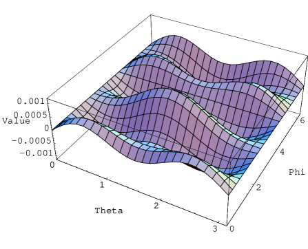
Figure 5: the angular dependence of the response function of the Virgo interferometer to the magnetic component of the $+$ polarization for $f=100Hz$

Figure 6: the angular dependence of the response function of the LIGO interferometer to the magnetic component of the $+$ polarization for $f=100Hz$

4 Analysis for the $\times$ polarization

The analysis can be generalized for the magnetic component of the $\times$ polarization too. In this case, equations (4) can be rewritten for the pure magnetic component of the $\times$ polarization as

$$\begin{array}[]{c}x(t)=l_{1}+\frac{1}{2}l_{2}l_{3}\dot{h}_{\times}(t)\\ \\ y(t)=l_{2}+\frac{1}{2}l_{1}l_{3}\dot{h}_{\times}(t)\\ \\ z(t)=l_{3}-\frac{1}{2}l_{1}l_{2}\dot{h}_{\times}(t).\end{array}$$ (18)

Using eqs. (18), (9) and (10), the $u$ coordinate of the mirror in the $u$ arm of the interferometer is given by

$$u=L+\frac{1}{4}L^{2}C\dot{h}_{\times}(t),$$ (19)

where

$$C\equiv-2\cos\theta\cos^{2}\phi\sin\theta\sin\phi,$$ (20)

while the $v$ coordinate of the mirror in the $v$ arm of the interferometer is given by

$$v=L+\frac{1}{4}L^{2}D\dot{h}_{\times}(t),$$ (21)

where

$$D\equiv 2\cos\theta\cos\phi\sin\theta\sin^{2}\phi.$$ (22)

Thus, with an analysis similar to the one of previous Sections, it is possible to show that the response function of the interferometer for the magnetic component of the $\times$ polarization is

$$\begin{array}[]{c}H_{magn}^{\times}(\omega)=-i\omega T(C-D)=\\ \\ =-i\omega L\sin 2\phi(\cos\phi+\sin\phi)\cos\theta,\end{array}$$ (23)

in perfect agreement with the result of Baskaran and Grishchuk (eqs. 46 and 50 of [24]). The absolute value of the total response functions (23) of the Virgo and LIGO interferometers to the magnetic component of the $\times$ polarization for $\theta=\frac{\pi}{4}$ and $\phi=\frac{\pi}{3}$ are respectively shown in figure 7 and 8 in the low- frequency range $10Hz\leq f\leq 100Hz$. This quantity increases with increasing frequency in analogy with the case shown in previous Section for the magnetic component of the $+$ polarization.

Figure 7: the absolute value of the total response function of the Virgo interferometer to the magnetic component of the $\times$ polarization for $\theta=\frac{\pi}{4}$ and $\phi=\frac{\pi}{3}$ in the low- frequency range $10Hz\leq f\leq 100Hz$

Figure 8: the absolute value of the total response function of the LIGO interferometer to the magnetic component of the $\times$ polarization for $\theta=\frac{\pi}{4}$ and $\phi=\frac{\pi}{3}$ in the low- frequency range $10Hz\leq f\leq 100Hz$

The angular dependences of the total response function (23) of the Virgo and LIGO interferometers to the magnetic component of the $\times$ polarization for $f=100Hz$ are shown in figure 9 and 10.

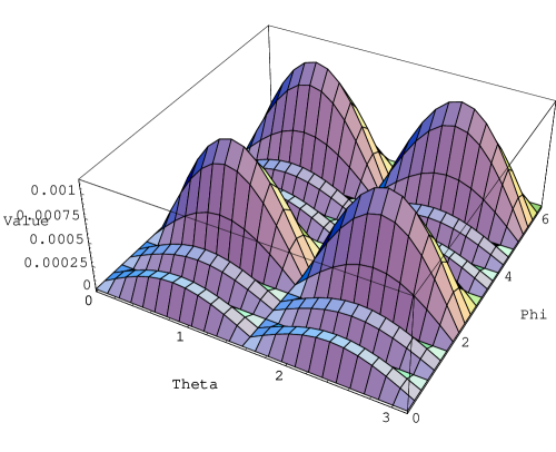
Figure 9: the angular dependence of the total response function of the Virgo interferometer to the magnetic component of the $\times$ polarization for $f=100Hz$

Figure 10: the angular dependence of the total response function of the LIGO interferometer to the magnetic component of the $\times$ polarization for $f=100Hz$

5 More accurate response functions for the magnetic components

One can extend equations (3) in the form [25, 27]

$$\begin{array}[]{c}t(t+z)=t_{tt}+\frac{1}{4}(x_{tt}^{2}-y_{tt}^{2})\dot{h}_{+}(t+z)-\frac{1}{2}x_{tt}y_{tt}\dot{h}_{\times}(t+z)\\ \\ x(t+z)=x_{tt}+\frac{1}{2}x_{tt}h_{+}(t+z)-\frac{1}{2}y_{tt}h_{\times}(t+z)+\frac{1}{2}x_{tt}z_{tt}\dot{h}_{+}(t+z)-\frac{1}{2}y_{tt}z_{tt}\dot{h}_{\times}(t+z)\\ \\ y(t+z)=y_{tt}+\frac{1}{2}y_{tt}h_{+}(t+z)-\frac{1}{2}x_{tt}h_{\times}(t+z)+\frac{1}{2}y_{tt}z_{tt}\dot{h}_{+}(t+z)-\frac{1}{2}x_{tt}z_{tt}\dot{h}_{\times}(t+z)\\ \\ z(t+z)=z_{tt}-\frac{1}{4}(x_{tt}^{2}-y_{tt}^{2})\dot{h}_{+}(t+z)+\frac{1}{2}x_{tt}y_{tt}\dot{h}_{\times}(t+z).\end{array}$$ (24)

This is because for a large separation between the test masses (in the case of Virgo the distance between the beam-splitter and the mirror is three kilometers, four in the case of LIGO), one cannot compute the coefficients of this transformation (components of the metric and its first time derivative) along the central wordline of the local observer, but a dependence from the position of the test masses is needed [25, 27]. Thus, also equations (4), (5), (6), (7), (8) and (11) have to be modified in the same way. In particular, we get

$$u=L+\frac{1}{4}L^{2}A\dot{h}_{+}(t+u\sin\theta\cos\phi).$$ (25)

From eq. (25) we find that the displacements of the two masses under the influence of the GW are

$$\delta u_{b}(t)=0$$ (26)

and

$$\delta u_{m}(t)=\frac{1}{4}L^{2}A\dot{h}_{+}(t+L\sin\theta\cos\phi).$$ (27)

In this way, the relative displacement, which is defined by

$$\delta L(t)=\delta u_{m}(t)-\delta u_{b}(t)$$ (28)

gives

$$\frac{\delta T(t)}{T}=\frac{\delta L(t)}{L}=\frac{1}{4}LA\dot{h}_{+}(t+L\sin\theta\cos\phi).$$ (29)

But we have the problem that, for the large separation between the test masses, the definition (28) for relative displacements becomes unphysical because the two test masses are taken at the same time and therefore cannot be in a casual connection [25, 27]. We can write the correct definitions using a the so called “bouncing photon method”: a photon can be launched from the beam-splitter to be bounced back by the mirror (Figure 1). This method has been generalized to scalar waves, angular dependences and massive modes of GWs in [2, 9, 25, 26, 27].

One obtains:

$$\delta L_{1}(t)=\delta u_{m}(t)-\delta u_{b}(t-T_{1})$$ (30)

and

$$\delta L_{2}(t)=\delta u_{m}(t-T_{2})-\delta u_{b}(t),$$ (31)

where $T_{1}$ and $T_{2}$ are the photon propagation times for the forward and return trip correspondingly. According to the new definitions, the displacement of one test mass is compared with the displacement of the other at a later time to allow for finite delay from the light propagation. We note that the propagation times $T_{1}$ and $T_{2}$ in eqs. (30) and (31) can be replaced with the nominal value $T$ because the test mass displacements are alredy first order in $h_{+}$ [25, 27]. Thus, for the total change in the distance between the beam splitter and the mirror in one round-trip of the photon, we get

$$\delta L_{r.t.}(t)=\delta L_{1}(t-T)+\delta L_{2}(t)=2\delta u_{m}(t-T)-\delta u_{b}(t)-\delta u_{b}(t-2T),$$ (32)

and in terms of the amplitude of the GW:

$$\delta L_{r.t.}(t)=\frac{1}{2}L^{2}A\dot{h}_{+}(t+L\sin\theta\cos\phi-L).$$ (33)

The change in distance (33) leads to changes in the round-trip time for photons propagating between the beam-splitter and the mirror:

$$\frac{\delta_{1}T(t)}{T}=\frac{1}{2}LA\dot{h}_{+}(t+L\sin\theta\cos\phi-L).$$ (34)

6 Effect of curved spacetime

In the last calculation (variations in the photon round-trip time which come from the motion of the test masses inducted by the magnetic component of the $+$ polarization of the GW), we implicitly assumed that the propagation of the photon between the beam-splitter and the mirror of the interferometer is uniform as if it were moving in a flat space-time. But the presence of the tidal forces indicates that the space-time is curved. As a result, we have to consider one more effect after the first discussed that requires spacial separation [25, 27].

From equation (27) we get the tidal acceleration of a test mass caused by the magnetic component of the $+$ polarization of the GW in the $u$ direction

$$\ddot{u}(t+u\sin\theta\cos\phi)=\frac{1}{4}L^{2}A\frac{\partial}{\partial t}\ddot{h}{}_{+}(t+u\sin\theta\cos\phi).$$ (35)

Equivalently, we can say that there is a gravitational potential [25, 27]:

$$V(u,t)=-\frac{1}{4}L^{2}A\int_{0}^{u}\frac{\partial}{\partial t}\ddot{h}{}_{+}(t+l\sin\theta\cos\phi)dl,$$ (36)

which generates the tidal forces, and that the motion of the test mass is governed by the Newtonian equation

$$\ddot{\overrightarrow{r}}=-\bigtriangledown V.$$ (37)

For the second effect, we consider the interval for photons propagating along the $u$ -axis

$$ds^{2}=g_{00}dt^{2}+du^{2}.$$ (38)

The condition for a null trajectory ($ds=0$) gives the coordinate velocity of the photons

$$v^{2}\equiv(\frac{du}{dt})^{2}=1+2V(t,u),$$ (39)

which to first order in $h_{+}$ is approximated by

$$v\approx\pm[1+V(t,u)],$$ (40)

with $+$ and $-$ for the forward and return trip respectively. If we know the coordinate velocity of the photon, we can define the propagation time for its travelling between the beam-splitter and the mirror:

$$T_{1}(t)=\int_{u_{b}(t-T_{1})}^{u_{m}(t)}\frac{du}{v}$$ (41)

and

$$T_{2}(t)=\int_{u_{m}(t-T_{2})}^{u_{b}(t)}\frac{(-du)}{v}.$$ (42)

The calculations of these integrals would be complicated because the $u_{m}$ boundaries of them are changing with time:

$$u_{b}(t)=0$$ (43)

and

$$u_{m}(t)=L+\delta u_{m}(t).$$ (44)

But we note that, to first order in $h{}_{+}$, these contributions can be approximated by $\delta L_{1}(t)$ and $\delta L_{2}(t)$ (see eqs. (30) and (31)). Thus, the combined effect of the varying boundaries is given by $\delta_{1}T(t)$ in eq. (34). Then, we have only to calculate the times for photon propagation between the fixed boundaries: $0$ and $L$. We will denote such propagation times with $\Delta T_{1,2}$ to distinguish from $T_{1,2}$. In the forward trip, the propagation time between the fixed limits is

$$\Delta T_{1}(t)=\int_{0}^{L}\frac{du}{v(t^{\prime},u)}\approx L-\int_{0}^{L}V(t^{\prime},u)du,$$ (45)

where $t^{\prime}$ is the delay time (i.e. $t$ is the time at which the photon arrives in the position $L$, so $L-u=t-t^{\prime}$) which corresponds to the unperturbed photon trajectory:

$t^{\prime}=t-(L-u)$.

Similarly, the propagation time in the return trip is

$$\Delta T_{2}(t)=L-\int_{L}^{0}V(t^{\prime},u)du,$$ (46)

where now the delay time is given by

$t^{\prime}=t-u$.

The sum of $\Delta T_{1}(t-T)$ and $\Delta T_{2}(t)$ give us the round-trip time for photons traveling between the fixed boundaries. Then, we obtain the deviation of this round-trip time (distance) from its unperturbed value $2T$:

$$\begin{array}[]{c}\delta_{2}T(t)=-\int_{0}^{L}[V(t-2L+u,u)du+\\ \\ -\int_{L}^{0}V(t-u,u)]du,\end{array}$$ (47)

and, using eq. (36), it is

$$\begin{array}[]{c}\delta_{2}T(t)=\frac{1}{4}L^{2}A\int_{0}^{L}[\int_{0}^{u}\frac{\partial}{\partial t}\ddot{h}_{+}(t-2T+l(1+\sin\theta\cos\phi))dl+\\ \\ -\int_{0}^{u}\frac{\partial}{\partial t}\ddot{h}_{+}(t-l(1-\sin\theta\cos\phi)dl]du.\end{array}$$ (48)

Thus, the total round-trip proper distance in presence of the magnetic component of the $+$ polarization of the GW is:

$$T_{t}=2T+\delta_{1}T+\delta_{2}T,$$ (49)

and

$$\delta T_{u}=T_{t}-2T=\delta_{1}T+\delta_{2}T$$ (50)

is the total variation of the proper time (distance) for the round-trip of the photon in presence of the magnetic component of the GW in the $u$ direction.

Using eqs. (34), (48) and the Fourier transform of $h_{+}$ defined by (16), the quantity (50) can be computed in the frequency domain:

$$\tilde{\delta}T_{u}(\omega)=\tilde{\delta}_{1}T(\omega)+\tilde{\delta}_{2}T(\omega)$$ (51)

where

$$\tilde{\delta}_{1}T(\omega)=-i\omega\exp[i\omega L(1-\sin\theta\cos\phi)]\frac{L^{2}A}{2}\tilde{h}_{+}(\omega)$$ (52)

$$\begin{array}[]{c}\tilde{\delta}_{2}T(\omega)=\frac{i\omega L^{2}A}{4}[\frac{-1+\exp[i\omega L(1-\sin\theta\cos\phi)]-iL\omega(1-\sin\theta\cos\phi)}{(1-\sin\theta\cos\phi)^{2}}+\\ \\ +\frac{\exp(2i\omega L)(1-\exp[i\omega L(-1-\sin\theta\cos\phi)]-iL\omega(1+\sin\theta\cos\phi)}{(-1-\sin\theta\cos\phi)^{2}}]\tilde{h}_{+}(\omega).\end{array}$$ (53)

In the above computation the derivation and translation theorems of the Fourier transform have been used. In this way, the response function of the $u$ arm of the interferometer to the magnetic component of the $+$ polarization of the GW is

$$\begin{array}[]{c}H_{u}^{+}(\omega)\equiv\frac{\tilde{\delta}T_{u}(\omega)}{L\tilde{h}_{+}(\omega)}=\\ \\ =-i\omega\exp[i\omega L(1-\sin\theta\cos\phi)]\frac{LA}{2}+\\ \\ \frac{i\omega LA}{4}[\frac{-1+\exp[i\omega L(1-\sin\theta\cos\phi)]-iL\omega(1-\sin\theta\cos\phi)}{(1-\sin\theta\cos\phi)^{2}}+\\ \\ +\frac{\exp(2i\omega L)(1-\exp[i\omega L(-1-\sin\theta\cos\phi)]-iL\omega(1+\sin\theta\cos\phi)}{(-1-\sin\theta\cos\phi)^{2}}].\end{array}$$ (54)

7 Computation for the $v$ arm

The computation for the $v$ arm is parallel to the one above. Using eqs. (8), (9) and (10) the coordinate of the mirror in the $v$ arm is:

$$v=L+\frac{1}{4}L^{2}B\dot{h}_{+}(t+v\sin\theta\sin\phi).$$ (55)

Thus, with the same way of thinking of previous Sections, we get variations in the photon round-trip time which come from the motion of the beam-splitter and the mirror in the $v$ direction:

$$\frac{\delta_{1}T(t)}{T}=\frac{1}{2}LB\dot{h}_{+}(t+L\sin\theta\sin\phi-L),$$ (56)

while the second contribute (propagation in a curve spacetime) will be

$$\begin{array}[]{c}\delta_{2}T(t)=\frac{1}{4}L^{2}B\int_{0}^{L}[\int_{0}^{u}\frac{\partial}{\partial t}\ddot{h}_{+}(t-2T+l(1-\sin\theta\sin\phi))dl+\\ \\ -\int_{0}^{u}\frac{\partial}{\partial t}\ddot{h}_{+}(t-l(1-\sin\theta\sin\phi)dl]du,\end{array}$$ (57)

and the total response function of the $v$ arm for the magnetic component of the $+$ polarization of GWs is given by

$$\begin{array}[]{c}H_{v}^{+}(\omega)\equiv\frac{\tilde{\delta}T_{u}(\omega)}{L\tilde{h}_{+}(\omega)}=\\ \\ =-i\omega\exp[i\omega L(1-\sin\theta\sin\phi)]\frac{LB}{2}+\\ \\ +\frac{i\omega LB}{4}[\frac{-1+\exp[i\omega L(1-\sin\theta\sin\phi)]-iL\omega(1-\sin\theta\sin\phi)}{(1-\sin\theta\cos\phi)^{2}}+\\ \\ +\frac{\exp(2i\omega L)(1-\exp[i\omega L(-1-\sin\theta\sin\phi)]-iL\omega(1+\sin\theta\sin\phi)}{(-1-\sin\theta\sin\phi)^{2}}].\end{array}$$ (58)

8 The total response function of an interferometer for the $+$ polarization

The total response function for the magnetic component of the $+$ polarization is given by the difference of the two response function of the two arms:

$$H_{tot}^{+}(\omega)\equiv H_{u}^{+}(\omega)-H_{v}^{+}(\omega),$$ (59)

and, using eqs. (54) and (58), we obtain a complicated formula

$$\begin{array}[]{c}H_{tot}^{+}(\omega)=\frac{\tilde{\delta}T_{tot}(\omega)}{L\tilde{h}_{+}(\omega)}=\\ \\ =-i\omega\exp[i\omega L(1-\sin\theta\cos\phi)]\frac{LA}{2}+\frac{LB}{2}i\omega\exp[i\omega L(1-\sin\theta\sin\phi)]\\ \\ -\frac{i\omega LA}{4}[\frac{-1+\exp[i\omega L(1-\sin\theta\cos\phi)]-iL\omega(1-\sin\theta\cos\phi)}{(1-\sin\theta\cos\phi)^{2}}\\ \\ +\frac{\exp(2i\omega L)(1-\exp[i\omega L(-1-\sin\theta\cos\phi)]-iL\omega(1+\sin\theta\cos\phi)}{(-1-\sin\theta\cos\phi)^{2}}]+\\ \\ +\frac{i\omega LB}{4}[\frac{-1+\exp[i\omega L(1-\sin\theta\sin\phi)]-iL\omega(1-\sin\theta\sin\phi)}{(1-\sin\theta\cos\phi)^{2}}+\\ \\ +\frac{\exp(2i\omega L)(1-\exp[i\omega L(-1-\sin\theta\sin\phi)]-iL\omega(1+\sin\theta\sin\phi)}{(-1-\sin\theta\sin\phi)^{2}}],\end{array}$$ (60)

that, in the low freuencies limit is in perfect agreement with the result of Baskaran and Grishchuk (eq. 49 of [24]), i.e. with eq. (17):

$$H_{tot}^{+}(\omega\rightarrow 0)=\frac{1}{4}\sin\theta[(\cos^{2}\theta+\sin 2\phi\frac{1+\cos^{2}\theta}{2})](\cos\phi-\sin\phi).$$ (61)

In figures 11 and 12 the angular dependences of the total response function (60) of the Virgo and LIGO interferometers to the magnetic component of the $+$ polarization of GWs at the frequency $f=8000Hz$ are respectively shown. This frequency falls in the high-frequency portion of the interferometers sensitivity band, thus, the “magnetic” contribution becomes quit important. In fact, figures 11 and 12 show that it can go over the 10% of the total signal.

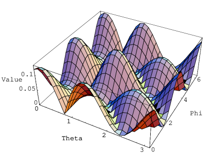
Figure 11: the angular dependence of the response function of the Virgo interferometer to the magnetic component of the $+$ polarization for $f=8000Hz$

Figure 12: the angular dependence of the response function of the LIGO interferometer to the magnetic component of the $+$ polarization for $f=8000Hz$

9 Analysis for the $\times$ polarization

The analysis can be generalized for the magnetic component of the $\times$ polarization too. In this case, using equations (24), (9) and (10) the $u$ coordinate of the mirror situated in the $u$ arm of the interferometer is given by

$$u=L+\frac{1}{4}L^{2}C\dot{h}_{\times}(t+u\sin\theta\cos\phi).$$ (62)

while the $v$ coordinate of the mirror situated in the $v$ arm of the interferometer is given by

$$v=L+\frac{1}{4}L^{2}D\dot{h}_{\times}(t+v\sin\theta\sin\phi).$$ (63)

Thus, with an analysis similar to the one of previous Sections, it is possible to show that the total response function of the interferometer for the magnetic component of the $\times$ polarization of GWs is

$$\begin{array}[]{c}H_{tot}^{\times}(\omega)=\frac{\tilde{\delta}T_{tot}(\omega)}{L\tilde{h}_{\times}(\omega)}=\\ \\ =-i\omega\exp[i\omega L(1-\sin\theta\cos\phi)]\frac{LC}{2}+\frac{LD}{2}i\omega\exp[i\omega L(1-\sin\theta\sin\phi)]\\ \\ -\frac{i\omega LC}{4}[\frac{-1+\exp[i\omega L(1-\sin\theta\cos\phi)]-iL\omega(1-\sin\theta\cos\phi)}{(1-\sin\theta\cos\phi)^{2}}\\ \\ +\frac{\exp(2i\omega L)(1-\exp[i\omega L(-1-\sin\theta\cos\phi)]-iL\omega(1+\sin\theta\cos\phi)}{(-1-\sin\theta\cos\phi)^{2}}]+\\ \\ +\frac{i\omega LD}{4}[\frac{-1+\exp[i\omega L(1-\sin\theta\sin\phi)]-iL\omega(1-\sin\theta\sin\phi)}{(1-\sin\theta\cos\phi)^{2}}+\\ \\ +\frac{\exp(2i\omega L)(1-\exp[i\omega L(-1-\sin\theta\sin\phi)]-iL\omega(1+\sin\theta\sin\phi)}{(-1-\sin\theta\sin\phi)^{2}}],\end{array}$$ (64)

that, in the low frequencies limit, is in perfect agreement with the result of Baskaran and Grishchuk (eq. 50 of [24]) and with eq. (23):

$$H_{tot}^{\times}(\omega\rightarrow 0)=\frac{1}{4}\sin 2\phi(\cos\phi+\sin\phi)\cos\theta.$$ (65)

In figure 13 and 14 the angular dependences of the total response function (64) of the Virgo and LIGO interferometers to the magnetic component of the $\times$ polarization of GWs at the frequency $f=8000Hz$ are respectively shown.

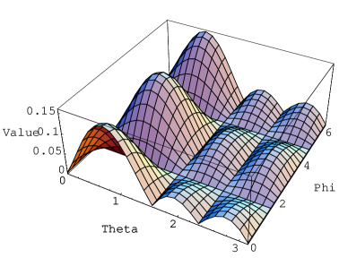
Figure 13: the angular dependence of the response function of the Virgo interferometer to the magnetic component of the $\times$ polarization for $f=8000Hz$

Figure 14: the angular dependence of the response function of the LIGO interferometer to the magnetic component of the $\times$ polarization for $f=8000Hz$

The figures show the importance of the “magnetic” contribution in the high-frequency portion of the interferometers sensitivity band in this case ($\times$ polarization) too.

Because the response functions to the “magnetic” components grow with frequency, as it is shown in eqs. (60) and (64), one could think that the part of signal which arises from the magnetic components could in principle become the dominant part of the signal at high frequencies (see also [25, 27]), and, in principle, extend the frequency range of interferometers. But, to understand if this is correct, one has to use the full theory of gravitational waves.

10 The total response function of interferometers in the full theory of gravitational waves

The low-frequencies approximation, used in Sections 3 and 4 to show that the “magnetic” and “electric” contributions to the response functions can be identified without ambiguity in the longh-wavelengths regime [26, 27, 24], is sufficient only for ground based interferometers, for which the condition $f\ll 1/L$ is in general satisfied. For space-based interferometers, for which the above condition is not satisfied in the high-frequency portion of the sensitivity band [24, 25, 26, 27], the response functions of Sections 8-9 give a better approximation [24, 25, 26, 27]. But, to compute the correct total response function, without any approximation in distance and/or frequency, the full theory of gravitational waves has to be used [2, 26].

In this Section, the variation of the proper distance that a photon covers to make a round-trip from the beam-splitter to the mirror of an interferometer is computed with the gauge choice (2) (see also [2, 26]). In this case, one does not need the coordinate transformation (3) from the TT coordinates to the frame of the local observer. Thus, with a treatment similar to the one of [2, 26], the analysis is translated in the frequency domain and the general response functions are obtained.

A special property of the TT gauge is that an inertial test mass initially at rest in these coordinates, remains at rest throughout the entire passage of the GW [2, 26]. Here we have to clarify the use of words “ at rest”: we want to mean that the coordinates of the test mass do not change in the presence of the GW. The proper distance between the beam-splitter and the mirror of the interferometer changes even though their coordinates remain the same [2, 26].

We start from the $+$ polarization. Labelling the coordinates of the TT gauge with $t,x,y,z$ for a sake of simplicity, the line element (2) becomes:

$$ds^{2}=-dt^{2}+dz^{2}+[1+h_{+}(t+z)]dx^{2}+[1+h_{+}(t+z)]dy^{2}.$$ (66)

But the arms of the interferometer are in the $\overrightarrow{u}$ and $\overrightarrow{v}$ directions, while the $x,y,z$ frame is the proper frame of the propagating GW.

The coordinate transformation for the metric tensor is [2, 26]:

$$g^{ik}=\frac{\partial x^{i}}{\partial x^{\prime l}}\frac{\partial x^{k}}{\partial x^{\prime m}}g^{\prime lm}.$$ (67)

By using eq. (9), (10) and (67), in the new rotated frame the line element (66) in the $\overrightarrow{u}$ direction becomes:

$$ds^{2}=-dt^{2}+[1+(\cos^{2}\theta\cos^{2}\phi-\sin^{2}\phi)h_{+}(t+u\sin\theta\cos\phi)]du^{2}.$$ (68)

The condition for null geodesics ($ds^{2}=0$) in eq. (68) gives the coordinate velocity of the photon:

$$v^{2}\equiv(\frac{du}{dt})^{2}=\frac{1}{[1+(\cos^{2}\theta\cos^{2}\phi-\sin^{2}\phi)h_{+}(t+u\sin\theta\cos\phi)]}.$$ (69)

We recall that the beam splitter is located in the origin of the new coordinate system (i.e. $u_{b}=0$, $v_{b}=0$, $w_{b}=0$). The coordinates of the beam-splitter $u_{b}=0$ and of the mirror $u_{m}=L$ do not change under the influence of the GW, thus, the duration of the forward trip can be written as

$$T_{1}(t)=\int_{0}^{L}\frac{du}{v(t^{\prime}+u\sin\theta\cos\phi)},$$ (70)

with

$t^{\prime}=t-(L-u)$.

In the last equation $t^{\prime}$ is the delay time (see Section 6).

At first order in $h_{+}$ this integral can be approximated with

$$T_{1}(t)=T+\frac{\cos^{2}\theta\cos^{2}\phi-\sin^{2}\phi}{2}\int_{0}^{L}h_{+}(t^{\prime}+u\sin\theta\cos\phi)du,$$ (71)

where

$T=L$

is the transit time of the photon in absence of the GW. Similiarly, the duration of the return trip will be

$$T_{2}(t)=T+\frac{\cos^{2}\theta\cos^{2}\phi-\sin^{2}\phi}{2}\int_{L}^{0}h_{+}(t^{\prime}+u\sin\theta\cos\phi)(-du),$$ (72)

though now the delay time is

$t^{\prime}=t-(u-l)$.

The round-trip time will be the sum of $T_{2}(t)$ and $T_{1}[t-T_{2}(t)]$. The latter can be approximated by $T_{1}(t-T)$ because the difference between the exact and the approximate values is second order in $h_{+}$. Then, to first order in $h_{+}$, the duration of the round-trip will be

$$T_{r.t.}(t)=T_{1}(t-T)+T_{2}(t).$$ (73)

By using eqs. (71) and (72) one sees immediately that deviations of this round-trip time (i.e. proper distance) from its unperturbed value are given by

$$\begin{array}[]{c}\delta T(t)=\frac{\cos^{2}\theta\cos^{2}\phi-\sin^{2}\phi}{2}\int_{0}^{L}[h_{+}(t-2T-u(1-\sin\theta\cos\phi))+\\ \\ +h_{+}(t+u(1+\sin\theta\cos\phi))]du.\end{array}$$ (74)

Now, using the Fourier transform of the $+$ polarization of the field, defined by eq. (16), one obtains in the frequency domain:

$$\delta\tilde{T}(\omega)=\frac{1}{2}(\cos^{2}\theta\cos^{2}\phi-\sin^{2}\phi)\tilde{H}_{u}(\omega,\theta,\phi)\tilde{h}_{+}(\omega),$$ (75)

where

$$\begin{array}[]{c}\tilde{H}_{u}(\omega,\theta,\phi)=\frac{-1+\exp(2i\omega L)}{2i\omega(1+\sin^{2}\theta\cos^{2}\phi)}+\\ \\ +\frac{-\sin\theta\cos\phi((1+\exp(2i\omega L)-2\exp i\omega L(1-\sin\theta\cos\phi)))}{2i\omega(1+\sin\theta\cos^{2}\phi)}\end{array}$$ (76)

and we immediately see that $\tilde{H}_{u}(\omega,\theta,\phi)\rightarrow L$ when $\omega\rightarrow 0$.

Thus, the total response function of the $u$ arm of the interferometer to the $+$ component is:

$$\Upsilon_{u}^{+}(\omega)=\frac{(\cos^{2}\theta\cos^{2}\phi-\sin^{2}\phi)}{2L}\tilde{H}_{u}(\omega,\theta,\phi),$$ (77)

where $2L=2T$ is the round-trip time in absence of gravitational waves.

In the same way, the line element (66) in the $\overrightarrow{v}$ direction becomes:

$$ds^{2}=-dt^{2}+[1+(\cos^{2}\theta\sin^{2}\phi-\cos^{2}\phi)h_{+}(t+v\sin\theta\sin\phi)]dv^{2},$$ (78)

and the response function of the $v$ arm of the interferometer to the $+$ polarization is:

$$\Upsilon_{v}^{+}(\omega)=\frac{(\cos^{2}\theta\sin^{2}\phi-\cos^{2}\phi)}{2L}\tilde{H}_{v}(\omega,\theta,\phi)$$ (79)

where, now

$$\begin{array}[]{c}\tilde{H}_{v}(\omega,\theta,\phi)=\frac{-1+\exp(2i\omega L)}{2i\omega(1+\sin^{2}\theta\sin^{2}\phi)}+\\ \\ +\frac{-\sin\theta\sin\phi((1+\exp(2i\omega L)-2\exp i\omega L(1-\sin\theta\sin\phi)))}{2i\omega(1+\sin^{2}\theta\sin^{2}\phi)},\end{array}$$ (80)

with $\tilde{H}_{v}(\omega,\theta,\phi)\rightarrow L$ when $\omega\rightarrow 0$. In this case the variation of the distance (time) is

$$\delta\tilde{T}(\omega)=\frac{1}{2}(\cos^{2}\theta\cos^{2}\phi-\cos^{2}\phi)\tilde{H}_{v}(\omega,\theta,\phi)\tilde{h}_{+}(\omega).$$ (81)

From equations (75) and (81), the total lengths of the two arms in presence of the $+$ polarization of the GW and in the frequency domain are:

$$\tilde{T}_{u}(\omega)=\frac{1}{2}(\cos^{2}\theta\cos^{2}\phi-\sin^{2}\phi)\tilde{H}_{u}(\omega,\theta,\phi)\tilde{h}_{+}(\omega)+T$$ (82)

and

$$\tilde{T}_{v}(\omega)=\frac{1}{2}(\cos^{2}\theta\cos^{2}\phi-\cos^{2}\phi)\tilde{H}_{v}(\omega,\theta,\phi)\tilde{h}_{+}(\omega)+T,$$ (83)

that are particular cases of the more general equation (39) in [24].

Thus, the total frequency-dependent response function (i.e. the detector pattern) of an interferometer to the $+$ polarization of the GW is:

$$\begin{array}[]{c}\tilde{H}^{+}(\omega)=\Upsilon_{u}^{+}(\omega)-\Upsilon_{v}^{+}(\omega)=\\ \\ =\frac{(\cos^{2}\theta\cos^{2}\phi-\sin^{2}\phi)}{2L}\tilde{H}_{u}(\omega,\theta,\phi)+\\ \\ -\frac{(\cos^{2}\theta\sin^{2}\phi-\cos^{2}\phi)}{2L}\tilde{H}_{v}(\omega,\theta,\phi)\end{array}$$ (84)

that, in the low frequencies limit ($\omega\rightarrow 0$) is in perfect agreement with the detector pattern of eq. (46) in [24], if one retains the first two terms of the expansion:

$$\begin{array}[]{c}\tilde{H}^{+}(\omega\rightarrow 0)=\frac{1}{2}(1+\cos^{2}\theta)\cos 2\phi+\\ \\ -\frac{1}{4}i\omega L\sin\theta[(\cos^{2}\theta+\sin 2\phi\frac{1+\cos^{2}\theta}{2})](\cos\phi-\sin\phi).\end{array}$$ (85)

This result also confirms that the magnetic contribution to the variation of the distance is an universal phenomenon because it has been obtained starting from the full theory of gravitational waves in the TT gauge (see also [2, 26, 27]).

The same analysis can be now performed for the $\times$ polarization. In this case, from eq. (2) the line element is:

$$ds^{2}=-dt^{2}+dz^{2}+dx^{2}+dy^{2}+2h_{\times}(t+z)dxdy,$$ (86)

and, by using eqs. (9), (10) and (67), the line element (86) in the $u$ direction and in the new rotated frame becomes:

$$ds^{2}=-dt^{2}+[1-2\cos\theta\cos\phi\sin\phi h_{\times}(t+u\sin\theta\cos\phi)]du^{2}.$$ (87)

Then, the response function of the $u$ arm of the interferometer to the $\times$ polarization is:

$$\Upsilon_{u}^{\times}(\omega)=\frac{-\cos\theta\cos\phi\sin\phi}{L}\tilde{H}_{u}(\omega,\theta,\phi),$$ (88)

while the line element (86) in the $v$ direction becomes:

$$ds^{2}=-dt^{2}+[1+2\cos\theta\cos\phi\sin\phi h_{\times}(t+u\sin\theta\sin\phi)]dv^{2}$$ (89)

and the response function of the $v$ arm of the interferometer to the $\times$ polarization is:

$$\Upsilon_{v}^{\times}(\omega)=\frac{\cos\theta\cos\phi\sin\phi}{L}\tilde{H}_{v}(\omega,\theta,\phi).$$ (90)

Thus, the total frequency-dependent response function of an interferometer to the $\times$ polarization is:

$$\tilde{H}^{\times}(\omega)=\frac{-\cos\theta\cos\phi\sin\phi}{L}[\tilde{H}_{u}(\omega,\theta,\phi)+\tilde{H}_{v}(\omega,\theta,\phi)],$$ (91)

that, in the low frequencies limit ($\omega\rightarrow 0$), is in perfect agreement with the detector pattern of eq. (46) of [24], if one retains the first two terms of the expansion:

$$\tilde{H}^{\times}(\omega\rightarrow 0)=-\cos\theta\sin 2\phi-i\omega L\sin 2\phi(\cos\phi+\sin\phi)\cos\theta.$$ (92)

The total lengths of the two arms in presence of the $\times$ polarization and in the frequency domain are:

$$\tilde{T}_{u}(\omega)=(\cos\theta\cos\phi\sin\phi)\tilde{H}_{u}(\omega,\theta,\phi)\tilde{h}_{\times}(\omega)+T$$ (93)

and

$$\tilde{T}_{v}(\omega)=(-\cos\theta\cos\phi\sin\phi)\tilde{H}_{v}(\omega,\theta,\phi)\tilde{h}_{\times}(\omega)+T,$$ (94)

that also are particular cases of the more general equation (39) of [24]. The total low frequencies response functions of eqs. (85) and (92) are more accurate than the “traditional” ones of [29, 30, 31], because our equations include the “magnetic” contribution.

Thus, the obtained results confirm the presence and importance of the so-called “magnetic” components of GWs and the fact that they have to be taken into account in the context of the total response functions of interferometers for GWs propagating from arbitrary directions.

The importance of the presented results is due to the fact that in this case the limit where the wavelenght is shorter than the lenght between the splitter mirror and test masses is calculated. The signal drops off the regime, while the calculation agrees with previous calculations for longer wavelenghts [24, 25]. The contribution is important expecially in the high-frequency portion of the sensitivity band.

In fact, one can see the pronounced difference between the “traditional” low-frequency approximation angular pattern of the Virgo interferometer for the $+$ polarization, i.e $\frac{1}{2}(1+\cos^{2}\theta)\cos 2\phi$ as it is computed in [29, 30, 31], which is shown in Figure 15, and the frequency-dependent angular pattern (84), which is shown in Figure 16 at a frequency of 8000 Hz, i.e. a frequency which falls in the high-frequency portion of the sensitivity band. The same angular patterns are shown in Figures 17 and 18 for the LIGO interferometer. The difference between the low-frequency approximation angular patterns and the frequency-dependent ones is important for the $\times$ polarization too, as it is shown in Figures 19, 20 for Virgo and in Figures 21, 22 for LIGO.

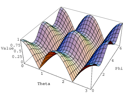
Figure 15: The low-frequency angular dependence to the $+$ polarization for the Virgo interferometer

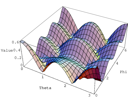
Figure 16: The angular dependence to the $+$ polarization for the Virgo interferometer at 8000 Hz

Figure 17: The low-frequency angular dependence to the $+$ polarization for the LIGO interferometer

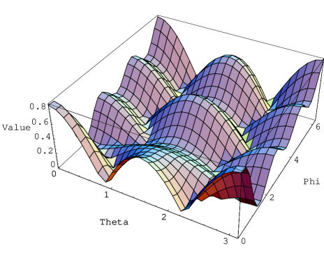
Figure 18: The angular dependence to the $+$ polarization for the LIGO interferometer at 8000 Hz

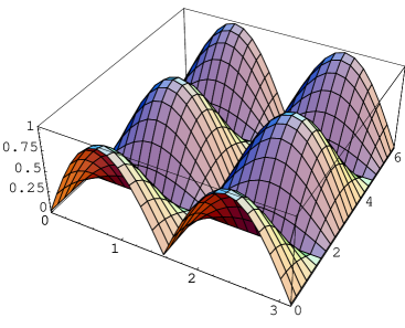
Figure 19: The low-frequency angular dependence to the $\times$ polarization for the Virgo interferometer

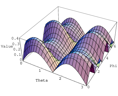
Figure 20: The angular dependence to the $\times$ polarization for the Virgo interferometer at 8000 Hz

Figure 21: The low-frequency angular dependence to the $\times$ polarization for the LIGO interferometer

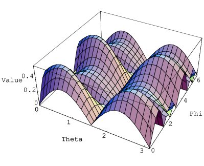
Figure 22: The angular dependence to the $\times$ polarization for the LIGO interferometer at 8000 Hz

Seeing the Figures 16 and 18 of eq. (84) and 20 and 22 of (91) at 8000 Hz, one sees that the magnetic component of GWs cannot extend the frequency range of interferometers. This is because, even if magnetic contributions grow with frequency, as it is shown from eq. (60), the division between “electric” and “magnetic” contributions breaks down at high frequencies, thus one has to perform computations using the full theory of gravitational waves. The correspondent response functions which are obtained do not grow which frequency.

11 Conclusions

Recently, arising from an enlighting analysis of Baskaran and Grishchuk in [24], some papers in the literature have shown the presence and importance of the so-called “magnetic” components of GWs, which have to be taken into account in the context of the total response functions of interferometers for GWs propagating from arbitrary directions. In [25] and [26] accurate response functions for the Virgo and LIGO interferometers have been analysed.

However, some results which have been shown in [25] look in contrast with the results which have been shown in[26]. In fact, in [25] it was claimed that the “magnetic” component of GWs could, in principle, extend the frequency range of Earth based interferometers, while in [26] such a possibility has been banned.

This contrast has been partially solved in [27].

The aim of this review paper has been to re-analyse all the framework of the “magnetic” components of GWs with the goal of solving the mentioned contrast in definitive way.

Accurate response funtions for the Virgo and LIGO interferometers have been re-discussed in detail too.

References

• [1] F. Acernese et al. (the Virgo Collaboration) - Class. Quant. Grav. 24, 19, S381-S388 (2007)
• [2] C. Corda - Astropart. Phys. 27, No 6, 539-549 (2007);
• [3] C. Corda - Int. J. Mod. Phys. D 16, 9, 1497-1517 (2007)
• [4] B. Willke et al. - Class. Quant. Grav. 23 8S207-S214 (2006)
• [5] D. Sigg (for the LIGO Scientific Collaboration) - www.ligo.org/pdf_public/P050036.pdf
• [6] B. Abbott et al. (the LIGO Scientific Collaboration) - Phys. Rev. D 72, 042002 (2005)
• [7] M. Ando and the TAMA Collaboration - Class. Quant. Grav. 19 7 1615-1621 (2002)
• [8] D. Tatsumi, Tsunesada Y and the TAMA Collaboration - Class. Quant. Grav. 21 5 S451-S456 (2004)
• [9] C. Corda - J. Cosmol. Astropart. Phys. JCAP04009 (2007)
• [10] C. Corda - Int. Journ. Mod. Phys. A 23, 10, 1521-1535 (2008)
• [11] G. Allemandi, M. Francaviglia, M. L. Ruggiero and A. Tartaglia - Gen. Rel. Grav. 37 11 (2005)
• [12] S. Capozziello and C. Corda - Int. J. Mod. Phys. D 15, 1119 -1150 (2006)
• [13] S. Capozziello, M. F. De Laurentis and M. Francaviglia - Astropart. Phys. 2, No 2, 125-129 (2008)
• [14] C. Corda- Astropart. Phys. 28, 247-250 (2007)
• [15] Allemandi G, Capone M, Capozziello S and Francaviglia M - Gen. Rev. Grav. 38 1 (2006)
• [16] Capozziello S and Francaviglia M - arXiv:0706.1146, to appear in Gen. Rel. Grav. (2007)
• [17] M. E. Tobar , T. Suzuki and K. Kuroda Phys. Rev. D 59 102002 (1999)
• [18] K. Nakao, T. Harada , M. Shibata, S. Kawamura and T. Nakamura - Phys. Rev. D 63, 082001 (2001)
• [19] C. Corda and M. F. De Laurentis - Proceedings of the 10th ICATPP Conference on Astroparticle, Particle, Space Physics, Detectors and Medical Physics - Applications, Villa Olmo, Como, Italy (October 8-12 2007)
• [20] C. Corda - Mod. Phys. Lett. A No. 22, 16, 1167-1173 (2007)
• [21] S. Capozziello, C. Corda and M. F. De Laurentis - Mod. Phys. Lett. A 22, 15, 1097-1104 (2007)
• [22] C. Corda - Mod. Phys. Lett. A No. 22, 23, 1727-1735 (2007)
• [23] C. Brans and R. H. Dicke - Phys. Rev. 124, 925 (1961)
• [24] D. Baskaran and L. P. Grishchuk - Class. Quant. Grav. 21 4041-4061 (2004)
• [25] C. Corda - Int. Journ. Mod. Phys. A 22, 13, 2361-2381 (2007)
• [26] C. Corda - Int. J. Mod. Phys. D 16, 9, 1497-1517 (2007)
• [27] C. Corda - Proceedings of the XLIInd Rencontres de Moriond, Gravitational Waves and Experimental Gravity, p. 95, Ed. J. Dumarchez and J. T. Tran, Than Van, THE GIOI Publishers (2007)
• [28] Misner CW, Thorne KS and Wheeler JA - “Gravitation” - W.H.Feeman and Company - 1973
• [29] Tinto M, Estabrook FB and Armstrong JW - Phys. Rev. D 65 084003 (2002)
• [30] Thorne KS - 300 Years of Gravitation - Ed. Hawking SW and Israel W Cambridge University Press p. 330 (1987)
• [31] Saulson P - Fundamental of Interferometric Gravitational Waves Detectors - World Scientific, Singapore (1994)