Dynamics of magnetization in frustrated spin-chain systems: Ca₃Co₂O₆

Abstract

The magnetization dynamics of the triangular lattice of Ising spin chains is investigated in the framework of a two-dimensional model. The rigid chains are assumed to interact with the nearest neighboring chains, an external magnetic field, and a heat reservoir that causes the chains to change their states randomly with time. A probability of a single spin-flip process is assumed in a Glauber-like form. This technique allows describing properly the steps in the magnetization curves observed in Ca₃Co₂O₆ and their dependence on a magnetic field sweep rate and temperature. A transition from a low-temperature to high-temperature phase is also observed.

Ising spin-chains packed into a two-dimensional (2D) frustrated lattice demonstrate a complex magnetic behavior due to a combination of a low dimensionality and frustration. There are few groups of compounds in which the triangular lattice is formed by antiferromagnetic (AFM) Ising spin chains, e.g. CsCoCl₃, CsCoBr₃ Mekata (1977), or ferromagnetic (FM) ones like Ca₃Co₂O₆ Aasland et al. (1997); Maignan et al. (2004). A spin-chain system Sr₅Rh₄O₁₂ discovered recently has a complex magnetic structure of chains Cao et al. (2007). An interaction between the nearest neighboring chains in the lattice is of the AFM type and much weaker than the intrachain one. However, it causes the frustration and a large variety of magnetic structures Mekata (1977); Aasland et al. (1997); Maignan et al. (2004); Cao et al. (2007); Kudasov (2006, 2007).

A step-like magnetization curve in Ca₃Co₂O₆ has drawn recently considerable attention Hardy et al. (2004a); Maignan et al. (2004); Hardy et al. (2004b, 2003); Maignan et al. (2000); Kudasov (2006, 2007); Petrenko et al. (2005); Kageyama et al. (1997); Fresard et al. (2004). The number of the steps depends on a sweep rate of the external magnetic field and temperature Maignan et al. (2004); Hardy et al. (2004b); Maignan et al. (2000). Two steps become apparent in the temperature range from 12 K to 24 K Maignan et al. (2000). The first step takes place at the zero magnetic field. Then a plateau at about $1/3$ of the full magnetization stretches up to the magnetic field of 3.6 T where the second step to the saturated FM state occurs. At least four equidistant steps are clearly visible below 12 K at a moderate magnetic field sweep rate Maignan et al. (2004); Hardy et al. (2004b). At an extremely low sweep rate the magnetization curve becomes close to the two-step shape, similar to that is observed at the high temperatures Hardy et al. (2004b). A response to alternating magnetic fields and its dependence on the temperature and magnetic field were investigated carefully in Ref.Hardy et al. (2004a). The experimental results show that there exist two characteristic time scales of the magnetization dynamics. The first is of order of 1 s and the second reaches a few hours.

A crystal structure of Ca₃Co₂O₆ consists of Co₂O₆ chains running along the $c$ axis. The Ca ions are situated between them and are not involved in magnetic interactions. The chains are made up of alternating face-sharing CoO₆ trigonal prisms and CoO₆ octahedra. The crystalline electric field splits the energy level of Co³⁺ ions into the high-spin ($S=2$) and low-spin ($S=0$) states. The chains form triangular lattice in the $ab$ plane that is perpendicular to the chains. An in-chain exchange interaction between high-spin cobalt ions through the octahedra with low-spin cobalt ions is ferromagnetic. The parameter of the FM in-chain coupling ($J_{F}$) was found from the magnetic susceptibility at high temperatures Kageyama et al. (1997), specific heat Hardy et al. (2003), and theoretical calculations Fresard et al. (2004). These estimations are in a reasonable agreement with each other ($J_{F}\approx 25$K). The weak AFM interchain interaction causes the partially disordered AFM (PDAFM) structure of chains (or honeycomb magnetic structure) below $T_{C1}$=24 K. At $T_{C2}\approx 12$ K another magnetic transition takes place Hardy et al. (2003); Petrenko et al. (2005). It should be mentioned that the topology of the magnetic net in Ca₃Co₂O₆ is rather complex, e.g. there exist helical paths Fresard et al. (2004).

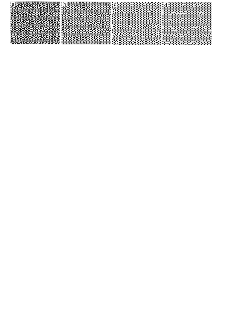
Figure 1: Fragments of the triangular lattice during the simulation at $T=4$ K and 1 T/min (from left to right): the initial state $B=0$ T, $B=0.768$ T, $B=1.824$ T, and $B=2.784$ T. The white and black circles stand for spin-up and spin-down chains.

Taking into account the strong intrachain interaction one can assume the chains to be in two ordered states (spin-up or spin-down) at low temperatures. This is a basic assumption of a rigid-chain model Kudasov (2006). Then the problem is reduced to the AFM triangular Ising model Wannier (1950); Kudasov (2006):

$$H=J\sum_{<ij>}{\sigma_{i}\sigma_{j}}-B\sum_{i}{\sigma_{i}}$$ (1)

where $\sigma_{i}=\pm{1}$ is the $c$-axis projection of the $i$-th chain spin, $J>0$ is the parameter of the AFM interchain coupling, $B$ is the external magnetic field, $<ij>$ denotes the summation over all the nearest-neighbor pairs on the triangular lattice.

A second assumption of the rigid-chain model is that even at a very low magnetic field sweep rate the system is out of equilibrium, i.e. it is in a metastable state rather than in the ground state Kudasov (2006). The large hysteresis loop and strong dependence of magnetization curve on the magnetic field sweep rate favor this point. Conditions of the metastability of the system can be formulated in the following form Kudasov (2006)

$$\sigma_{i}h_{i}\leq 0$$ (2)

where $h_{i}=J\sum_{<ij>}{\sigma_{j}}-B$ is the effective field for the $i$-th chain. This inequality should be satisfied for all the chains. Following the single-flip technique for the nonequilibrium Ising model Kim et al. (2003) the probability $W_{i}$ of a spin-flip event at the $i$-th chain was formulated as

$$W_{i}=\left\{\begin{array}[]{cc}0&\text{ if }\sigma_{i}h_{i}<0,\\ 1&\text{ if }\sigma_{i}h_{i}\geq 0.\end{array}\right.$$ (5)

The rigid-chain model describes properly the four-step magnetization curve in Ca₃Co₂O₆. On the other hand one should keep in mind that once the system occurs in a metastable state it will dwell in this state for an arbitrarily long time, i.e. this is a frozen metastability approximation.

Recently, static magnetization curves in Ca₃Co₂O₆ were investigated by means of Monte Carlo technique Yao et al. (2006). It was observed that the perfect triangular lattice of the rigid spins produces the two-step magnetization curve even at low temperatures. To overcome this problem the nearest-neighbor interactions were radomized. The magnetization curves demonstrated the four-step behavior on such imperfect lattice. However, it should be pointed out that these two types of the magnetization curves were observed experimentally on the same sample at different sweep rates Hardy et al. (2004b). Therefore the four-step magnetization curve can not originate from the lattice imperfection.

In the present paper, we generalize the rigid-chain model to include dynamical aspects of the problem. Following to the Glauber theory Glauber (1963) we assume that the chains interact not only with the nearest neighbors and external magnetic field but also with a heat reservoir. In this case the probability of a spin flip of the $i$-th chain per time unit can be written down as

$$W_{i}=\frac{\alpha}{2}\left[1-\sigma\cdot\tanh\left(-\frac{J}{kT}\sum_{<ij>}\sigma{{}_{j}}+\frac{\mu B}{kT}\right)\right]$$ (6)

where $\alpha$ is the constant of the interaction of a chain with the heat reservoir, $k$ is the Boltzmann constant, $T$ is the temperature, $\mu$ is the chain magnetization. It should be mentioned that the ratio $J/\mu$ do not depend on the chain length. It is determined by the plateau length in the magnetization curve ($\Delta B=1.2$ T for Ca₃Co₂O₆). In effect a temperature behavior of the system is related to the effective temperature $kT/N$ where $N$ is the length of the chain (number of magnetic ions).

One can see that if $T\rightarrow 0$ the expression (6) goes to the function (5), i.e. the model of Ref.Kudasov (2006) is the low-temperature limit of the present one. In the opposite case $T\rightarrow\infty$ the probability of a spin-flip event is independent on the magnetic field and interchain coupling. At finite temperatures the probability depends on the ratio of the effective field to the temperature and is nonzero even if $\sigma_{i}h_{i}<0$. That is why, an evolution of metastable states exists within this model.

We have performed a numerical simulation of the magnetization evolution on a rhombic $96{\times}\,96$ supercell of the triangular lattice with periodic boundary conditions. Few periodic structures can appear during the simulation. To avoid artificial domain boundaries the length of the supercell should be multiple of a periodicity of these structures. In order to satisfy this condition for any three- or two-sublattice ordering the length was chosen to be multiple of 6. Preliminary calculations on $24{\times}\,24$, $48{\times}\,48$ , and $192{\times}\,192$ supercells showed a good convergence of the results. The best coincidence of the theoretical and experimental data occurred at $\alpha=0.21$ s^-1 and $N=30$ which are reasonable values. They were used in all further calculations.

The simulation started with preparation of an initial state. As it was discussed in Ref.Kudasov (2006) the PDAFM structure is rather close to the ground state of the AFM triangular Ising model. That is why, the initial state was obtained by an evolution of the PDAFM phase at the zero magnetic field. When the duration of this preliminary evolution was more than $5\alpha^{-1}$, results of the simulation became practically independent on the initial state. The typical duration of the preliminary evolution in our calculations was about $100\alpha^{-1}$. A fragment of the initial state is shown in Fig.1a. It should be mentioned that one can prepare the initial state from an arbitrary random state. However it requires a longer period to get the initial state.

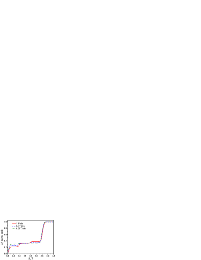
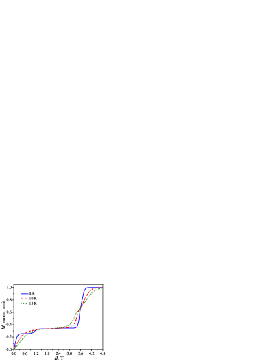
Figure 2: The magnetization curves in the increasing magnetic field at different sweep rates and $T=4$ K (left) and at different temperatures with the constant magnetic field field sweep rate of $0.1$ T/min (right).

After obtaining the initial state the magnetic field was switched on at a constant sweep rate. We adjusted the magnetic field sweep rates to the experimental values of Ref.Hardy et al. (2004b). A typical number of time steps was about $2\cdot 10^{6}$ per a full cycle (increasing-field and decreasing-field branches).

Fig. 2 demonstrates an average magnetic moment as a function of magnetic field $M(B)$ calculated for different magnetic field sweep rates at a constant temperature (in the left panel) and for different temperatures at a constant sweep rate (in the right panel). One can see that the second and third steps in the magnetization curve vanish with decreasing of the magnetic field sweep rate or with increasing the temperature. This general tendency and shape of the magnetization curves are in a very good agreement with the experimental observations Hardy et al. (2004b).

To clarify an origin of such behavior we present specimens of configurations at different magnetic fields corresponding to the plateaus in the magnetization curves at the highest magnetic field sweep rate (see Fig.1). One can clearly see domains in the figures. The ferrimagnetic state is formed by three sublattice. It is obviously three-fold degenerate. While the magnetic field sweep rate is sufficiently fast the ferrimagnetic phase starts growing at a number of nucleation centers. This causes the domain formation. With a decrease of the sweep rate the domains expand and for the extremely slow sweep rate the domain walls almost disappear. It is easy to see that the single-domain ferrimagnetic state leads to the two-step magnetization curve because all the spin-down chains are encircled by six spin-up chains. The dotted curve in the left panel of Fig.2 corresponding to the extremely low magnetic field sweep rate is similar to that was obtained by the Monte Carlo technique Yao et al. (2006).

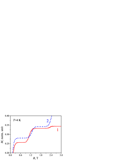
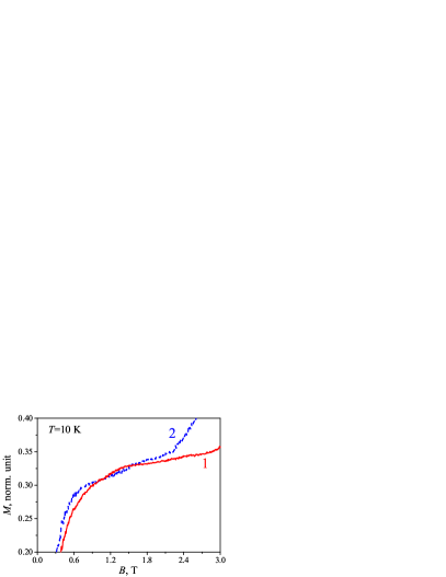
Figure 3: Enlargements of hysteresis loops with a sweep rate of $0.1$ T/min at $4$ K and $10$ K. The solid lines and dashed lines are the field-increasing and field-decreasing branches, respectively.

Domain boundaries contain chains with other environments and cause appearance of the two additional steps in the magnetization curve. For instance, at the first plateau (Fig.1b) there are spin-down chains with 2 spin-down and 4 spin-up nearest neighbors. Their critical spin-flip field is 1.2 T. At the second plateau (Fig.1c) there exist spin-down chains with 1 spin-down and 5 spin-up nearest neighbors. Their critical spin-flip field is 2.4 T. The higher the magnetic field sweep rate is, the smaller the domains become and the more apparent the additional magnetization steps are.

Here we should mention that the chains in the domain boundaries as well as the internal chains are in metastable states at the plateaus, that is, they are oriented along the effective fields. The spin-flip probability in the form of Eq.(6) allows some fraction of exited states that, in their turn, leads to a creep of the domain wall. This is a new important ingredient which appears in the present theory. It explains the existence of two characteristic times in Ca₃Co₂O₆. The first one is related to a single spin-flip evens and specifies the fast processes of about 1 s. The second is due to the creep of the domain boundaries (up to 10⁴ s).

As it was argued in Ref.Kudasov (2007) the transition from the low-temperature to high-temperature regime stems from disordering of a fraction of the chains. This mechanism is essentially three-dimensional. That is why, the observation of this transition within the present 2D model is surprising. The present interpretation of the transition differs from that was assumed in Ref.Kudasov (2007). It arises due to a drastic increase of a domain boundary mobility at high temperatures that leads to establishing of the single-domain ferrimagnetic state during a short time.

Another interesting features that were observed experimentally are crossings of field-increasing and field-decreasing branches of the magnetization curve Hardy et al. (2004b). As one can see in Fig.3 they are also reproduced by the simulations.

In conclusion, in the present paper we go beyond the frozen metastability approximation of Ref.Kudasov (2006). The simulation of the nonequilibrium evolution was performed by means of a Glauber-like form of the spin-flip probability that allows us investigating the dependence of the magnetization curves on the temperature and magnetic field sweep rate in a good agreement with the experimental data. At the extremely low magnetic field sweep rate the results of the 2D simulation are similar to that was obtained by the Monte Carlo technique Yao et al. (2006). The present model gives reasonable values of both the critical temperatures: $T_{C2}\approx 10$ K and $T_{C1}\approx 20$ K. Although it is not valid at high temperatures ($T\gtrsim 15$ K) since the intrachain disorder becomes essential Kudasov (2007). An experimental feature that escapes the 2D simulation is a drastic increase of the hysteresis loop at a very low temperature ($T=2$ K) as compared to moderate temperatures ($T\sim 5$ K). Most probably it is related to an intrachain dynamics of the magnetization and requires a 3D simulation to be describe properly.

The work was supported by ISTC (project # 3501), RFBR (projects 08-02-97018-r-povolzhje-a, 08-02-00508-a), and Federal Agency of Science and Innovations of Russian Federation. D.A.M. acknowledges a support of the “Dynasty” foundation.

References

- Mekata (1977) M. Mekata, J. Phys. Soc. Jpn. 42, 76 (1977).
- Aasland et al. (1997) S. Aasland, H. Fjellvag, and B. Hauback, Sol. St. Comm. 101, 187 (1997).
- Maignan et al. (2004) A. Maignan, V. Hardy, S.Hebert, M. Drillon, M. R. Lees, O. Petrenko, D. M. K. Paul, and D. Khomskii, J. Mater. Chem. 14, 1231 (2004).
- Cao et al. (2007) G. Cao, V. Durairaj, S. Chikara, S. Parkin, and P. Schlottmann, Phys. Rev. B 75, 134402 (2007).
- Kudasov (2006) Y. B. Kudasov, Phys. Rev. Lett. 96, 27212 (2006).
- Kudasov (2007) Y. B. Kudasov, EPL 78, 57005 (2007).
- Hardy et al. (2004a) V. Hardy, D. Flahaut, M. R. Lees, and O. A. Petrenko, Phys. Rev. B 70, 214439 (2004a).
- Hardy et al. (2004b) V. Hardy, M. R. Lees, O. A. Petrenko, D. M. K. Paul, D. Flahaut, S.Hebert, and A. Maignan, Phys. Rev. B 70, 64424 (2004b).
- Hardy et al. (2003) V. Hardy, S. Lambert, M. R. Lees, and D. M. K. Paul, Phys. Rev. B 68, 14424 (2003).
- Maignan et al. (2000) A. Maignan, C. Michel, A. C. Masset, C. Martin, and B. Raveau, Europ. Phys. Jour. B 15, 657 (2000).
- Kageyama et al. (1997) H. Kageyama, K. Yoshimura, K. Kosuge, H. Mitamura, and T. Goto, J. Phys. Soc. Jpn. 66, 3996 (1997).
- Fresard et al. (2004) R. Fresard, C. Laschinger, T. Kopp, and V. Eyert, Phys. Rev. B 69, 140405 (2004).
- Petrenko et al. (2005) O. A. Petrenko, J. Wooldridge, M. R. Lees, P. Manuel, and V. Hardy, Eur. Phys. Jour. B 47, 79 (2005).
- Wannier (1950) G. H. Wannier, Phys. Rev. 79, 357 (1950).
- Kim et al. (2003) E. Kim, B. Kim, and S. Lee, Phys. Rev. E 68, 66127 (2003).
- Yao et al. (2006) X. Yao, S. Dong, and J.-M. Liu, Phys. Rev. B 73, 212415 (2006).
- Glauber (1963) R. Glauber, Jour. Mat. Phys 2, 294 (1963).