Second-order shaped pulses for solid-state quantum computation

Abstract

We present the construction and detailed analysis of highly-optimized self-refocusing pulse shapes for several rotation angles. We characterize the constructed pulses by the coefficients appearing in the Magnus expansion up to second order. This allows a semi-analytical analysis of the performance of the constructed shapes in sequences and composite pulses by computing the corresponding leading-order error operators. Higher orders can be analyzed with the numerical technique suggested by us previously. We illustrate the technique by analyzing several composite pulses designed to protect against pulse amplitude errors, and on decoupling sequences for potentially long chains of qubits with on-site and nearest-neighbor couplings.

I Introduction

The implementation of quantum algorithms using NMR on molecules in liquidVandersypen et al. (2001), solidLeskowitz et al. (2003), and liquid crystalsYannoni et al. (1999) has demonstrated in principle that pulse-based control methods can be useful for quantum information processingVandersypen and Chuang (2004) (QIP). The technique has long been a staple in NMR spectroscopy, where complex molecules like proteins are analyzed with the help of long sequences of precisely designed radiofrequency pulsesSlichter (1992). Related techniques for coherent manipulation of many-body quantum systems have emerged as an important tool in many areas of science and technology.

A useful quantum computer should contain hundreds, if not thousands of qubits. The only hope of scaling to such system sizes is with the help of multiple levels of quantum error correction (QEC). For this to work, the benefits due to each additional level of encoding should outweigh the corresponding overhead of additional errors. This leads to various threshold theoremsKnill et al. (1998); Fowler et al. (2004), estimating the maximum error rate for which such concatenated encoding can be beneficial. The corresponding thresholds are rather stringent, meaning that for scalability one needs very accurate elementary gates.

Even for relatively small $n$-body systems, the number of states scales exponentially with $n$, and the accuracy required for QIP is high. As demonstrated in several recent experiments in NMR QIP, required accuracy can be reached with the help of strongly-modulating pulses, where entire single- or few-qubit gates are designed numerically for a given moleculePrice et al. (2000); Boulant et al. (2003) [also see Sanders et al., 1999; Hodgkinson et al., 2000; Niskanen et al., 2003; Steffen and Koch, 2007]. While the technique indeed offers unprecedentedly accurate, fast gates (which also helps to avoid relaxation), it obviously cannot be generalized to larger systems.

In contrast, the traditional pulse and sequence design rely on the Magnus (cumulant) expansionSlichter (1992). The expansion is done around the evolution in the applied controlling fields, while the chemical shiftsWarren (1984); Bauer et al. (1984); Geen and Freeman (1991) (resonant-frequency offsets) and inter-qubit couplings are treated perturbatively. The main advantage of the Magnus expansion is its locality. Namely, when local qubit couplings are dominant, the control fields accurate to a given order can be designed by analyzing relatively small clusters. The results remain exact independent of the system size, or even in the limit of infinite system. One can thus characterize pulse-based method for designing control fields as scalable to large system sizes. Goswami (2003).

A scheme to systematically construct high-order self-refocusing pulses and pulse sequences was developed by the authors in Ref. Sengupta and Pryadko, 2005. Specifically, we constructed “soft” NMR-styleWarren (1984); Freeman (1998) second-order self-refocusing inversion ($\pi$) pulses and several high-order sequences based on such pulses for refocusing qubits arranged in spin chains with on-site chemical shifts and XXZ nearest-neighbor coupling. The main technical advance which enabled the calculationsSengupta and Pryadko (2005) was the efficient numerical algorithm for computing high-order terms of the Magnus expansion. The algorithm is based on the usual time-dependent perturbation theory; the direct computation of multiple integrals entering higher-order cumulants would be totally impossible.

In this paper we present highly-optimized self-refocusing pulse shapes for rotation angles $\phi_{0}$ other than 180^∘. For such pulses, we extend the results of Ref. Pryadko and Quiroz, 2007 and construct the analytical expansion of the evolution operator for an arbitrary coupled qubit. While the expansion is more complicated than that for the inversion pulses with $\phi_{0}=180^{\circ}$, to second order, it is still characterized by only three coefficients, two of which we suppress by pulse shaping. This allows us to compute the error operators associated with a given control sequence semi-analytically, by evaluating the leading order terms in the corresponding products of the evolution operators. We illustrate the technique on several newly-constructed decoupling sequences for a chain of qubits with on-site and nearest-neighbor couplings, as well as with the composite pulses protecting against amplitude errors.

II Problem setup

II.1 Dynamical Decoupling

In principle, the simplest type of control pulses consist of short, intense bursts of coherent, resonant electromagnetic radiation, popularly known as “hard” or “bang-bang” pulses. In this limit, for the duration $\tau$ of the pulse one can totally ignore all other couplings of the qubit(s). Then, a pulse sequence can be viewed as a series of free evolution intervals [unitary evolution operators $U_{f}(t)=\exp(-itH_{S})$, where $H_{S}$ is the system Hamiltonian] intercalated with pulse operators. For example, with single-qubit control Hamiltonian,

$$H_{C}={1\over 2}\sum_{a}V^{\mu}_{a}(t)\sigma^{\mu}_{a},$$ (1)

where $\sigma^{\mu}_{a}$, $\mu=x,y,z$ are the Pauli matrices for $a$-th qubit and $V^{\mu}_{a}(t)$ are the corresponding control fields (or, more precisely, the envelopes of the control fields applied at the resonant frequency of the corresponding qubit), the pulse operator is the product of those for individual qubits, $P=\prod_{a}P_{a}(\phi_{0}^{(a)},\hat{\bf n}_{a})$,

$$P_{a}(\phi_{0},{\bf n})=\cos{\phi_{0}\over 2}-i\hat{\bf n}\cdot\vec{\sigma}_{a}\sin{\phi_{0}\over 2}.$$ (2)

Here $\hat{\bf n}$ is the unit vector that determines the spin rotation axis and $\phi_{0}$ is the corresponding angle,

$$\phi_{0}\,\hat{\bf n}^{\mu}=\int_{0}^{\tau}dt\,V^{\mu}(t).$$

The corresponding pulse algebra is straightforward. For example, for a single spin with the chemical shift Hamiltonian,

$$H_{S}={\Delta\over 2}\,\sigma^{z},$$ (3)

the sequence of two equally-spaced inversion pulses ($\phi_{0}=\pm\pi$) in $x$-direction is equivalent to a unitary,

$$P(\pi,\hat{\bf x})\,U_{f}(t)\,P(-\pi,\hat{\bf x})\,U_{f}(t)$$ (4)

$$=(-i\sigma^{x})\,\exp\Bigl{(}-i{t\Delta\over 2}\sigma^{z}\Bigr{)}(i\sigma^{x})\,\exp\Bigl{(}-i{t\Delta\over 2}\sigma^{z}\Bigr{)}$$

$$=\exp\Bigl{(}+i{t\Delta\over 2}\sigma^{z}\Bigr{)}\exp\Bigl{(}-i{t\Delta\over 2}\sigma^{z}\Bigr{)}=\openone,$$

which is, of course, the formal identity behind the well-known spin-echo sequenceHahn (1950).

In reality, the pulse duration $\tau$ is always finite. Thus, during the pulse application, the rotation actually happens around the axis determined by the sum of the system and control Hamiltonians; one gets finite-pulse-duration errors. Generically, such errors scale linearly with pulse duration. These errors are especially dangerous in systems where one cannot reduce the pulse duration indefinitely, e.g., because of the need for spectral addressing in homonuclear NMR, or in order to avoid exciting levels outside the qubit state in Josephson phase qubitsSteffen et al. (2003). Yet, even in systems with optical qubit coupling where $\tau$ could be in the sub-picosecond range, the finite-pulse-duration errors can be significant if one targets the accuracy necessary for achieving the scalability thresholdsChen et al. (2001).

The finite-pulse-duration errors can be significantly reduced by suppressing the leading-order error operators. The errors would scale with a higher power of the pulse duration, which makes them much more manageable. This can be achieved either by designing special sequences (which typically doubles or quadruples the number of pulses), or by using specially designed self-refocusing pulse shapesWarren (1984). Typically, the latter strategy is more efficientSengupta and Pryadko (2005); besides, the self-refocusing pulses can often be used as drop-in replacements for corresponding $\delta$-pulsesSengupta and Pryadko (2005); Pryadko and Quiroz (2007).

II.2 Model

We consider the following simplified Hamiltonian

$$H(t)=H_{\rm C}(t)+H_{\rm S}+H_{V}(t)+H_{\sigma},$$ (5)

with the first (main) term due to individual control fields,

$$H_{\rm C}(t)={1\over 2}\sum_{n}\bigl{[}V^{x}_{n}(t)\,\sigma^{x}_{n}+V^{y}_{n}(t)\,\sigma^{y}_{n}\bigr{]},$$ (6)

where $\sigma_{n}^{\mu}$, $\mu=x,y,z$, are the usual Pauli matrices for the $n$-th qubit (spin) of the 1D chain. The other terms include the native Hamiltonian of the system

$$H_{\rm S}={1\over 2}\sum_{n}\Delta_{n}^{\mu}\sigma_{n}^{\mu}+{1\over 4}\sum_{n<m}J_{nm}^{\mu\nu}\sigma_{n}^{\nu}\sigma_{m}^{\mu}+\ldots$$ (7)

describing the constant qubit couplings and the interactions between the qubits, and the coupling with the oscillator thermal bath,

$$H_{V}(t)={\textstyle\sum}_{n\mu}A_{n}^{\mu}\,V_{n}^{\mu}(t),\quad H_{\sigma}={1\over 2}{\textstyle\sum}_{n}B_{n}^{\mu}\,\sigma^{\mu}_{n}.$$ (8)

In Eq. (8), $A_{n}^{\mu}\equiv A_{n}^{\mu}(p_{i},q_{i})$ account for the possibility of a direct coupling of the controlling fields $V_{n}^{\mu}$ with the bath variables $q_{i}$, $p_{i}$, while $B_{n}^{\mu}\equiv B_{n}^{\mu}(p_{i},q_{i})$ describe the usual coupling of the spins with the oscillator bath. Already in the linear response approximation, the bath couplings (8) produce a frequency-dependent renormalization of the control Hamiltonian $H_{\rm C}(t)$ [Eq. (6)], as well as the thermal bath heating via the dissipative part of the corresponding response function. Both effects become more of a problem with increased spectral width of the controlling signals $V_{n}^{\mu}$. In this work we do not specify the explicit form of the coupling $H_{V}(t)$. Instead, we minimize the spectral width of the constructed pulses.

While the Hamiltonian (7) is a generic spin Hamiltonian, we will also consider specifically the Hamiltonian of XXZ model with additional on-site fields,

$$H_{\rm S}^{XXZ} = {1\over 4}\sum_{\langle n,n^{\prime}\rangle}\bigl{[}J_{n,n^{\prime}}^{z}\sigma^{z}_{n}\sigma^{z}_{n^{\prime}}+J_{n,n^{\prime}}^{\perp}(\sigma^{x}_{n}\sigma^{x}_{n^{\prime}}+\sigma^{y}_{n}\sigma^{y}_{n^{\prime}})\bigr{]}$$ (9)

$$+{1\over 2}\sum_{n,\mu}\Delta_{n}^{\mu}\sigma_{n}^{\mu}.$$

II.3 Magnus expansion

In a qubit-only system with the Hamiltonian

$$H(t)=H_{\rm C}(t)+H_{\rm S},$$ (10)

the effect of the applied fields is fully described by the evolution operator $U(t)$,

$$U(t)\equiv T\exp\Biglb(-i\int_{0}^{t}dt^{\prime}\,H(t^{\prime})\Bigrb),\quad$$ (11)

where $T$ is the Dyson time ordering operator.

For pulses with finite width, any desired unitary transformation can only be implemented approximately. A widely used framework to design pulses to effect a desired unitary transformation (or, equivalently, remove the effect of undesired terms in the Hamiltonian) is the MagnusMehring (1983) expansion and the average Hamiltonian theoryWaugh et al. (1968a, b). The expansion is done with respect to the evolution due to the control fields alone,

$$U_{0}(t)=T\exp\Biglb(-i\int_{0}^{t}dt^{\prime}\,H_{C}(t^{\prime})\Bigrb),$$ (12)

by defining the system Hamiltonian in the interaction representation (the “rotating-frame Hamiltonian”),

$${\tilde{H}}_{S}(t) = U_{0}^{\dagger}(t)H_{S}U_{0}(t).$$ (13)

For a periodic control field, $H_{1}(t+\tau_{c})=H_{1}(t)$, such that the zeroth-order driven evolution is also periodic, $U_{0}(t+\tau_{c})=U_{0}(t)$, one has the following expansion in powers of $\tau_{c}$:

$$U(n\tau_{c}) = \exp(-i{\bar{H}}\,n\tau_{c}),$$ (14)

$$\bar{H} = {\bar{H}}^{(0)}+{\bar{H}}^{(1)}+{\bar{H}}^{(2)}+\ldots,$$ (15)

where

$${\bar{H}}^{(0)}\tau_{c} = \int_{0}^{\tau_{c}}dt\,{\tilde{H}}_{1},$$ (16)

$${\bar{H}}^{(1)}\tau_{c} = -{i\over 2}\int_{0}^{\tau_{c}}dt_{2}\int_{0}^{t_{2}}dt_{1}\,[{\tilde{H}}_{2},{\tilde{H}}_{1}],$$ (17)

$${\bar{H}}^{(2)}\tau_{c} = -{1\over 6}\int_{0}^{\tau_{c}}dt_{3}\int_{0}^{t_{3}}dt_{2}\int_{0}^{t_{2}}dt_{1}$$ (19)

$$\times\left([{\tilde{H}}_{3},[{\tilde{H}}_{2},{\tilde{H}}_{1}]]+[{\tilde{H}}_{1},[{\tilde{H}}_{2},{\tilde{H}}_{3}]]\right).$$

Generally, the term ${\bar{H}}^{(k-1)}$ contains a $k$-fold integration of the commutators of the rotating-frame Hamiltonian $\tilde{H}_{i}\equiv\tilde{H}_{\rm S}(t_{i})$ at different time moments $t_{i}$ and scales as $\|{\bar{H}}^{(k)}\|\tau_{c}\propto\|\tau_{c}H_{\rm S}\|^{k}$. Note that for small enough $\tau_{c}$, the expansion parameter remains small even for long evolution time.

The Magnus expansion thus offers a basis for constructing successful approximations towards the desired unitary evolution. With the simpler problem of decoupling, the goal is to have no evolution. A $K$-th order refocusing sequence can be defined as that where there is no evolution to $K$-th order, that is,

$$\bar{H}^{(0)}=\bar{H}^{(1)}=\ldots=\bar{H}^{(K-1)}=0.$$ (20)

Respectively, at time $n\tau_{c}$, the error in the unitary evolution operator would scale as $\|U(n\tau_{c})-\openone\|\propto n\|\tau_{c}H_{\rm S}\|^{K+1}$, and the corresponding fidelity $F(t)$ differs from unity by

$$1-F(n\tau_{c})\propto n^{2}\|\tau_{c}H_{\rm S}\|^{2K+2}.$$ (21)

A crucial advantage of the cumulant expansion is that the cumulants do not contain the disconnected terms arising from different parts of the system (cluster theoremDomb and Green (1974); G. A. Baker (1990)). For an arbitrary lattice model of the form (9), with bonds representing the qubit interactions, the terms contributing to $k$-th order can be represented graphically as connected clusters involving up to $k$ lattice bonds; for a chain of qubit such clusters cannot have more than $n=k+1$ vertices. Thus, to obtain the exact form of the expansion up to and including $K$-th order, one needs to analyze all distinct chain clusters with up to $K+1$ vertices.

II.4 Time dependent perturbation theory

While the Magnus expansion is conceptually straightforward, it is cumbersome to implement and, most importantly, the repeated integrations are very expensive computationally already at the second order, see Eq. (17). An alternative strategy for evaluating high-order terms of the Magnus expansion was suggested by the present authors in Ref. Sengupta and Pryadko, 2005. Instead of working with the cumulants, the technique is based on the time-dependent perturbation theory (TDPT). The expansion is done around the non-perturbed evolution due to control fields alone, see Eq. (12). However, for actual computations, it is more convenient to use the differential equation

$$\dot{U}_{0}(t)=-iH_{C}(t)\,U_{0}(t),\quad U_{0}(0)=\openone.$$ (22)

The slow evolution operator

$$R(t)=U_{0}^{\dagger}(t)\,U(t).$$ (23)

obeys the equation

$$\dot{R}(t)=-i\tilde{H}_{S}(t)R(t),\quad\tilde{H}_{\rm S}(t)\equiv U_{0}^{\dagger}(t)\,H_{\rm S}\,U_{0}(t),$$ (24)

which can be iterated to construct the standard expansion $R(t)=\mathbb{I}+R_{1}(t)+R_{2}(t)+\ldots$ in powers of $(t\,H_{\rm S})$,

$$\dot{R}_{k}(t)=-i\tilde{H}_{S}(t)R_{k-1}(t),\quad R_{0}(t)={\mathbb{I}}.$$ (25)

The successive terms can be evaluated by solving, at each step, a set of coupled first order ODE’s simultaneously. For a finite system of $n$ qubits and a given maximum order $K$ of the expansion, one needs to solve Eqs. (22) and (25) with $1\leq k\leq K$. These are total of $(K+1)$ coupled systems of first order ordinary differential equations for the $2^{n}\times 2^{n}$ matrices $U_{0}$, $R_{1}$, $R_{2}$, …, $R_{K}$, and can be integrated efficiently. Computationally, this is a much less challenging job than that of evaluating repeated integrals (17), (19), and higher order terms. For a given system, solving the full set of equations (24) is simpler by a factor of at least $(K+1)$. However, it is the analysis of the perturbative expansion that is the key for achieving the scalability of the results.

Given the set of computed $R_{k}(\tau_{c})\equiv R_{k}$, the standard Magnus expansion can be readily obtained by taking the logarithm of the series,

$$-iH^{(0)}\tau_{c} = R_{1},$$ (26)

$$-iH^{(1)}\tau_{c} = R_{2}-{1\over 2}R_{1}^{2},$$ (27)

$$-iH^{(2)}\tau_{c} = R_{3}-{1\over 2}\bigl{[}R_{1}R_{2}+R_{2}R_{1}\bigr{]}+{1\over 3}R_{1}^{3},\,\ldots.$$ (28)

Obviously, the order-$K$ universal self-refocusing condition (20) is formally equivalent to

$$R_{1}(\tau_{c})=R_{2}(\tau_{c})=\ldots=R_{K}(\tau_{c})=0.$$ (29)

The matrices $R_{k}$ in the latter condition are much easier to evaluate numerically using Eqs. (22), (25). Importantly, the benefits of the cluster theorem are retained: to $K$-th order only clusters with up to $K+1$ vertices need to be analyzed.

III Pulse design and analysis

III.1 Pulse design using TDPT

The shapes of NMR-style one-dimensional pulsesWarren (1984), self-refocusing to a given order, can be found by analyzing the single-spin dynamics with the system Hamiltonian (3) and the control Hamiltonian

$$H_{C}(t)={1\over 2}\sigma^{x}V(t).$$ (30)

Specifically, we encoded the trial pulse shapes in terms of their Fourier coefficients,

$${V(t)}={\phi_{0}\over\tau}+\Omega\sum_{m}A_{m}\cos\biglb(m\Omega(t-\tau/2)\bigrb),$$ (31)

where $\tau$ is the pulse duration, $\Omega\equiv 2\pi/\tau$ is the corresponding angular frequency, and $\phi_{0}$ is the requested rotation angle of the pulse. Note that the form (31) guarantees the symmetry of the pulse, $V(\tau-t)=V(t)$. In addition, in order to reduce the spectral width of the control fields, we also constrained a certain number of derivatives of the function (31) to vanish at $t=0$ and $t=\tau$, $V^{(l)}(0)=0$, $l=0,1,\ldots,2L-1$.

We implemented the computational algorithm described in the previous section using the standard fourth-order Runge-Kutta algorithm for solving coupled differential equations  (22), (25), and the GSL libraryGalassi et al. (2003) for matrix operations. The coefficient optimization was done using a combination of simulated annealing and the steepest descent method. The target function for single-pulse optimization included the sum of the magnitudes squared of the matrix elements of the matrices $R_{k}\equiv R_{k}(\tau)$, $k=1,\ldots,K$, as well as the weighed sum of the squares of the coefficients $A_{m}$,

$$f_{K}=\left(\sum_{k=1}^{K}\mathop{\rm tr}R_{k}^{\dagger}R_{k}\right)^{1/2}+\epsilon\sum_{m=1}^{M}m^{2}A_{m}^{2}.$$ (32)

The second sum serves to provide some suppression of the higher Fourier harmonics of the pulse. In our simulations, the minimization was considered as having converged only after the first term evaluated to zero with numerical precision (typically, eight digits or better). For such a minimum to exist, the coefficient $\epsilon$ in Eq. (32) should be sufficiently small (we used $\epsilon=10^{-4}$).

For given pulse order $K$ and the given number of additional constraints $L$, there is a minimum number of harmonics $M_{\mathrm{min}}(K,L)$ necessary for convergence. However, we found that the shapes obtained with $M=M_{\mathrm{min}}(K,L)$ tend be over constrained and simply do not look nice. Our solution was to add one or two additional Fourier harmonics by increasing $M$.

III.2 Pulse shapes

Previously, in Ref. Sengupta and Pryadko, 2005, we gave the coefficients of the first-order self-refocusing ($K=1$) inversion ($\phi_{0}=\pi$) pulse shapes $S_{L}$, as well as the second-order ($K=2$) inversion shapes $Q_{L}$, $L=1,2$. Here $L$ is the parameter that indicates the number of constraints at the ends of the interval: the value of the function and its derivatives up to $(2L-1)$st vanish at the ends of the interval [note that all odd derivatives are suppressed automatically due to the symmetry of the function, see Eq. (31)].

In this work, we extend the list of constructed pulses to rotation angles $\phi_{0}=10^{\circ}$, $20^{\circ}$, …, $180^{\circ}$. In Table  1, we list the coefficients for the pulses used in the simulations. The coefficients for all of the constructed pulses are available upon request.

	$A_{0}$	$A_{1}$	$A_{2}$	$A_{3}$	$A_{4}$	$A_{5}$
$S_{1}(2\pi)$	1.0	-0.0237996956	-0.6226198703	-0.3535804341
$S_{2}(2\pi)$	1.0	-0.0294359406	-1.1741824154	-0.2097531295	0.4133714855
$Q_{1}(2\pi)$	1.0	2.1406171699	-2.3966480505	-0.6474844418	-0.0964846776
$Q_{2}(2\pi)$	1.0	1.4818894659	-2.6971749102	-0.4384679067	0.3434236044	0.3103297466
$S_{1}\equiv S_{1}(\pi)$	0.5	-1.2053193822	0.4796467863	0.2256725959
$S_{2}\equiv S_{2}(\pi)$	0.5	-1.1950692860	0.7841592117	0.0737326786	-0.1628226043
$Q_{1}\equiv Q_{1}(\pi)$	0.5	-1.1374072085	1.5774920785	-0.6825355002	-0.2575493698
$Q_{2}\equiv Q_{2}(\pi)$	0.5	-1.0964843348	1.5308987822	-1.1472441408	0.0025173181	0.2103123753
$S_{1}(\pi/2)$	0.25	-1.8963102551	1.1337663752	0.5125438801
$S_{2}(\pi/2)$	0.25	-1.9049987341	1.9858884053	0.1063314501	-0.4372211211
$Q_{1}(\pi/2)$	0.25	-1.8948543589	0.5873324062	0.5970352560	0.4604866969
$Q_{2}(\pi/2)$	0.25	-2.1145695246	0.6415685732	1.6854185871	0.4511145740	-0.9135322049

Table 1: Fourier coefficients for the constructed pulses, see Eq. (31). Shapes $S_{L}(\phi_{0})$ and $Q_{L}(\phi_{0})$ are the pulse shapes for rotation angle $\phi_{0}$, respectively first ($K=1$) and second ($K=2$) order for the Hamiltonian (3). These shapes have $2L$ derivatives vanishing at the ends of the interval.

(a)
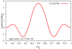
(b)
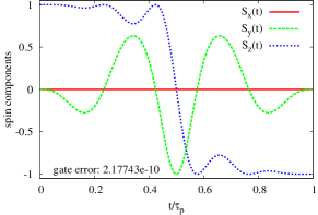
(c)

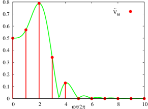
Figure 1: A single-spin second-order inversion ($\pi$) pulse $Q_{1}(\pi)$. (a) Pulse profile over a complete period, (b) Evolution of the spin beginning with $s_{z}=1$. (c) The power spectrum of the pulse. The vertical lines denote the location of the harmonics. As seen, the spectral weight is almost entirely confined to $\omega<5\omega_{0}$.

(a)
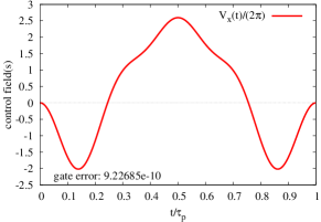
(b)
(c)

Figure 2: As in Fig. 1, but for the single-spin second-order $\pi/2$ pulse $Q_{1}(\pi/2)$.

Figure 3: (color online) Pulse shapes for $\phi_{0}=\pi/2$. Solid lines represent $Q_{L}(\pi/2)$, dashed lines correspond to $S_{L}(\pi/2)$. Pulse shapes with $L=1$ are drawn with thin blue lines, while those with $L=2$ are drawn with thick red lines. The black doted line shows the Gaussian shape $G_{010}(\pi/2)$.

Figure 4: (color online) As in Fig. 3 but for the inversion pulses, $\phi_{0}=\pi$. Note that the 1st order pulses ($S_{L}(\pi)$, dashed lines) actually have a smaller power than the Gaussian pulse.

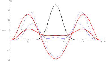
Figure 5: (color online) As in Fig. 3 but for the pulses with $\phi_{0}=2\pi$. The pulse shapes appear to resemble those of a pair of consecutive $\pi$ pulses. Second-order pulses happen to have the smallest power.

III.3 Pulse shape analysis

The pulse shapes $Q_{L}(\phi_{0})$, $S_{L}(\phi_{0})$ are constructed as first- or second-order self-refocusing pulses for the chemical shift Hamiltonian, Eq. (3). We would like, however, to have a universally good pulse shape that would work in most settings. To analyze the performance of the constructed pulses in most general circumstances, we construct the Magnus expansion of the evolution operator for the most general system Hamiltonian,

$$H_{S}=A_{0}+A_{x}\sigma^{x}+A_{y}\sigma^{y}+A_{z}\sigma^{z},$$ (33)

where $A_{\mu}$ are the operators responsible for coupling with the outside worlds, and $A_{0}$ is the external Hamiltonian. The analysis of the inversion pulses with $\phi_{0}=\pi$ appeared previously in Ref. Pryadko and Quiroz, 2007; here we extend it to $\phi_{0}\neq\pi$.

III.3.1 Driven evolution

The control Hamiltonian (30) alone [to zeroth order in $H_{S}$] produces the following unitary evolution operator [cf. Eq. (12)]

$$U_{0}(t)=e^{-i\sigma^{x}\phi(t)/2},\quad\phi(t)\equiv\int_{0}^{t}dt^{\prime}\,V(t^{\prime}).$$ (34)

When acting on the spin operators, this is just a rotation, $U_{0}^{\dagger}(t)\sigma^{y}U_{0}(t)=\sigma^{y}\cos\phi(t)-\sigma^{z}\sin\phi(t)$. Consequently, the system Hamiltonian in the interaction representation has the form

$$\tilde{H}_{S}(t) = A_{0}+\sigma^{x}A_{x}+\sigma^{y}(A_{y}\cos\phi+A_{z}\sin\phi)$$ (35)

$$+\sigma^{z}(A_{z}\cos\phi-A_{y}\sin\phi).$$

III.3.2 Leading-order average Hamiltonian

The zeroth order average Hamiltonian (17) is just the average of Eq. (35) over the pulse duration. We assume $V(t)$ represents a symmetric pulse, $V(\tau_{p}-t)=V_{x}(t)$. Then, $\phi(t)$ is antisymmetric, $\phi(\tau_{p}-t)=\phi_{0}-\phi(t)$, where $\phi_{0}\equiv\phi(\tau_{p})$ is the overall notation angle. It is convenient to introduce the symmetrized rotation angle,

$$\varphi(t)\equiv\phi(t)-\phi_{0}/2,$$ (36)

such that $\varphi(\tau_{p}-t)=-\varphi(\tau_{p})$. Then, the average of the sine over the pulse duration vanishes, $\langle\sin\varphi\rangle=0$. This implies that the averages of the cosine and sine of the original rotation angle are

$$\overline{\tt c} \equiv \langle\cos\phi\rangle=\cos(\phi_{0}/2)\langle\cos\varphi\rangle,$$ (37)

$$\overline{\tt s} \equiv \langle\sin\phi\rangle=\sin(\phi_{0}/2)\langle\cos\varphi\rangle,$$ (38)

where

$$\langle f(t)\rangle\equiv{1\over\tau_{p}}\int_{0}^{\tau_{p}}dt\,f(t).$$ (39)

If we denote

$$\upsilon\equiv\langle\cos\varphi\rangle=\int_{0}^{\tau_{p}}{dt\over\tau_{p}}\cos\varphi(t),$$ (40)

then the zeroth order average Hamiltonian for a one-dimensional pulse becomes

$$\bar{H}^{(0)} = A_{0}+\sigma^{x}A_{x}+\upsilon\Bigr{[}\sigma^{y}\Bigl{(}A_{y}\cos{\phi_{0}\over 2}+A_{z}\sin{\phi_{0}\over 2}\Bigr{)}$$ (41)

$$+\sigma^{z}\Bigl{(}A_{z}\cos{\phi_{0}\over 2}-A_{y}\sin{\phi_{0}\over 2}\Bigr{)}\Bigr{]}.$$

For the special case of the chemical-shift Hamiltonian (3), we have $A_{0}=A_{x}=A_{y}=0$, $A_{z}=\Delta/2$, and Eq. (41) gives

$$\bar{H}^{(0)}=\upsilon{\Delta\over 2}\left(\sigma^{z}\cos{\phi_{0}\over 2}+\sigma^{y}\sin{\phi_{0}\over 2}\right).$$ (42)

Clearly, the 1st-order self-refocusing condition corresponds to $\upsilon=0$. For such pulses the full zeroth-order average Hamiltonian is given just by the two first terms in Eq. (42).

III.3.3 1st-order average Hamiltonian

The 1st-order average Hamiltonian (17) is given by a double integral of the commutator of the system Hamiltonian in the interaction representation (35) evaluated at two different times. We note that every term in Eq. (35) can be classified as either time-independent [proportional to $e(t)\equiv 1$], proportional to $c(t)\equiv\cos\phi(t)$, or to $s(t)\equiv\sin\phi(t)$. Therefore, most generally, the second-order terms in the evolution operator can contain the following nine integrals,

$$\overline{\tt ee}\equiv\langle 1^{\prime}1\rangle={1\over 2}, \!\!\overline{\tt ec}\equiv\langle 1^{\prime}\cos\phi\rangle,\quad\overline{\tt es}\equiv\langle 1^{\prime}\sin\phi\rangle,$$

$$\!\!\overline{\tt ce}\equiv\langle\cos\phi^{\prime}\,1\rangle,\quad\overline{\tt se}\equiv\langle\sin\phi^{\prime}\,1\rangle,$$

$$\overline{\tt cc}\equiv\langle\cos\phi^{\prime}\cos\phi\rangle, \!\!\overline{\tt cs}\equiv\langle\cos\phi^{\prime}\sin\phi\rangle,$$

$$\overline{\tt sc}\equiv\langle\sin\phi^{\prime}\cos\phi\rangle, \!\!\overline{\tt ss}\equiv\langle\sin\phi^{\prime}\sin\phi\rangle,$$ (43)

where we used the notation

$$\langle f(\phi^{\prime})g(\phi)\rangle\equiv{1\over\tau^{2}}\int_{0}^{\tau}dt^{\prime}\,f\biglb(\phi(t^{\prime})\bigrb)\int_{0}^{t^{\prime}}dt\,g\biglb(\phi(t)\bigrb),$$ (44)

and $1\equiv e(t)$ or $1^{\prime}\equiv e(t^{\prime})$ indicate an identity factor at the corresponding position of the average. However, because of the commutator structure in Eq. (17), only the following antisymmetric combinations appear in the expression for the corresponding term in the average Hamiltonian theory, $H^{(1)}$,

$${\alpha\over 2}\equiv{\overline{\tt sc}-\overline{\tt cs}\over 2},\quad\zeta_{C}\equiv{\overline{\tt ec}-\overline{\tt ce}\over 2},\quad\zeta_{S}\equiv{\overline{\tt es}-\overline{\tt se}\over 2},$$ (45)

where

$$\alpha\equiv{1\over 2\tau_{p}^{2}}\int_{0}^{\tau_{p}}dt^{\prime}\int_{0}^{t^{\prime}}dt\,\sin\biglb(\phi(t^{\prime})-\phi(t)\bigrb)$$ (46)

In fact, the coefficients $\zeta_{C}$ and $\zeta_{S}$ can be reduced further,

$$\zeta_{C}=\zeta\sin{\phi_{0}\over 2},\quad\zeta_{S}=-\zeta\cos{\phi_{0}\over 2},$$ (47)

where [see Eq. (36) for the definition of $\varphi(t)$]

$$\zeta\equiv\int_{0}^{\tau_{p}}{dt^{\prime}\over\tau_{p}}\Bigl{(}{t\over\tau_{p}}-{1\over 2}\Bigr{)}\sin\varphi(t).$$ (48)

Thus, to second order, the average Hamiltonian of a symmetric angle-$\phi_{0}$ one-dimensional pulse is determined by only three dimensionless coefficients, $\upsilon$, $\alpha$, and $\zeta$, see Eqs. (40), (46), and (48). These coefficients contain all the relevant information about the shape of the pulse.

An explicit calculation of the 1st-order average Hamiltonian gives

$$H^{(1)} = \alpha\tau_{p}(i[A_{z},A_{y}]-\sigma^{x}(A_{y}^{2}+A_{z}^{2}))$$

$$+ \zeta\tau_{p}\cos{\phi_{0}\over 2}\Biglb(\sigma^{y}(i[A_{z},A_{0}]+\{A_{x},A_{y}\})+\sigma^{z}(i[A_{0},A_{y}]+\{A_{x}.A_{z}\})\Bigrb)$$

$$- \zeta\tau_{p}\sin{\phi_{0}\over 2}\Biglb(\sigma^{y}(i[A_{y},A_{0}]-\{A_{x},A_{z}\})+\sigma^{z}(i[A_{z},A_{0}]+\{A_{x},A_{y}\})\Bigrb).\hskip 216.81pt$$

For the Hamiltonian (3), the terms with $\zeta$ disappear, and we have, simply

$$H^{(1)}=-\alpha\sigma_{x}{\Delta^{2}\tau_{p}\over 4}.$$ (49)

Thus, the second-order self-refocusing pulses have both $\upsilon=0$ and $\alpha=0$.

The actual parameters for the pulses with $\phi_{0}=\pi/2$, $\pi$, and $2\pi$ are listed in TAB. 2.

pulse	$\phi_{0}$	$\upsilon\equiv\langle\cos\varphi\rangle$	$\alpha$	$\zeta$
$\phi_{0}\delta(t-\tau_{p}/2)$	$\phi_{0}$	$\displaystyle\cos{\phi_{0}\over 2}$	$\displaystyle{\sin\phi_{0}\over 4}$	$\displaystyle{1\over 4}\sin{\phi_{0}\over 2}$
$\displaystyle{\pi\over 2}\delta(t-\tau_{p}/2)$	$\pi/2$	$\sqrt{2}/2$	$1/4$	$\sqrt{2}/8$
$G_{0.05}[90]$	${\pi}/{2}$	$0.730111$	$0.398519$	$0.175999$
$G_{0.1}(90)$	${\pi/2}$	$0.753116$	$0.420275$	$0.173665$
$S_{1}(90)$	$\pi/2$	$0$	$-0.013067$	$0.198719$
$S_{2}(90)$	$\pi/2$	$0$	$-0.0294665$	$0.182109$
$Q_{1}(90)$	$\pi/2$	$0$	$0$	$0.202067$
$Q_{2}(90)$	$\pi/2$	$0$	$0$	$0.161658$
$\displaystyle{\pi}(t-\tau_{p}/2)$	$\pi$	$0$	$0$	$1/4$
$G_{0.05}(180)$	$\pi$	$0.0744894$	$0.0377451$	$0.249476$
$G_{0.1}(180)$	$\pi$	$0.148979$	$0.0764911$	$0.247905$
$S_{1}(180)$	$\pi$	$0$	$0.0332661$	$0.238227$
$S_{2}(180)$	$\pi$	$0$	$0.0250318$	$0.241378$
$Q_{1}(180)$	$\pi$	$0$	$0$	$0.239888$
$Q_{2}(180)$	$\pi$	$0$	$0$	$0.242209$
$\displaystyle{2\pi}(t-\tau_{p}/2)$	$2\pi$	$-1$	$0$	$0$
$G_{0.05}(360)$	$2\pi$	$-0.896959$	$0.402852$	$0.00291436$
$G_{0.1}(360)$	$2\pi$	$-0.793918$	$0.317488$	$0.0116577$
$S_{1}(360)$	$2\pi$	$0$	$0.0739621$	$0.113233$
$S_{2}(360)$	$2\pi$	$0$	$0.0612747$	$0.0811486$
$Q_{1}(360)$	$2\pi$	$0$	$0$	$0.00403872$
$Q_{2}(360)$	$2\pi$	$0$	$0$	$0.00734526$

Table 2: Parameters of several common pulse shapes. The first line represents the “hard” $\delta$-function pulse applied at the center of the interval of duration $\tau$, $G_{001}$ denotes the Gaussian pulse with the width $0.01\tau_{p}$, while $S_{n}$ and $Q_{n}$ denote the 1st and 2nd-order self-refocusing pulses from Tab. 1.

IV Open systems

In this work we concentrate on the performance of high-order pulses and pulse sequences in closed quantum systems. However, it turns out that such sequences also remain efficient in open systems, in the presence of low-frequency bath modesPryadko and Sengupta (2006); Pryadko and Quiroz (2007).

The analysis is done in general form with the help of an assumption that the bath couplings have the same form as the existing terms in the system Hamiltonian (7), which are assumed to be suppressed to order $K=1$ or $K=2$. The bath modes are assumed to be low-frequency; in addition to the expansion in powers of the corresponding couplings, one needs a low frequency expansion in powers of the adiabaticity parameter $\tau_{c}/\tau_{0}$, where $\tau_{c}$ is the decoupling cycle duration and $\tau_{0}$ is the bath correlation time.

With $K=1$ decoupling, the effect in the open system is a suppression of direct decay ($T_{1}$) processes, as well as the reduction of the dephasing rate ($T_{2}$) by the factor of order of the adiabaticity parameter $\tau_{c}/\tau_{0}$. The former result can be understood by analyzing the spectral properties of the driven systemKofman and Kurizki (2001, 2004), while the latter can be viewed as due to a reduction of the time step for phase diffusion. With second-order decoupling, $K=2$, the decoherence rate is additionally suppressed, and with time-reversal invariant bath coupling all orders of the expansion in powers of adiabaticity parameter may vanish, in which case the leading-order dephasing term becomes exponentially small and dephasing would likely be determined by terms of higher order in bath coupling. Along with the decoherence rates characterizing the exponential decay of quantum correlations with time, the corresponding prefactor, which determines the “visibility” (or “initial decoherence”Facchi et al. (2005)), was also analyzedPryadko and Sengupta (2006). While for generic refocusing sequences with $K\geq 1$ the initial decoherence is quadratic in $\tau_{c}$ and does not scale with the thermal bath correlation time $\tau_{0}$, for symmetric pulse sequences it is reduced by an additional power of the adiabaticity parameter $(\tau/\tau_{0})$. These results were originally derived for a generic featureless bath, but they also hold in a vicinity of a sharp resonance as long as the effective (i.e., renormalized as in the average Hamiltonian) coupling to the corresponding mode is small compared to its widthPryadko and Quiroz (2007).

V Application examples.

V.1 Decoupling sequences for a chain of qubits

Decoupling sequences are designed to prevent quantum evolution from happening. Thus, we want to construct a sequence such that the resulting evolution operator over the period $\tau_{c}$ is identity, $U(\tau_{c})=\openone$. We illustrate the scalability of dynamical decoupling to large system sizes by considering linear chains of qubits with either Ising or XXZ n.n. random-valued couplings [only $J_{n,n+1}^{z}$ or both $J_{n,n+1}^{z}$ and $J_{n,n+1}^{x}=J_{n,n+1}^{y}$ in Eq. (7)], plus the local fields either along $z$ axis or in arbitrary direction [$\Delta^{z}_{n}\neq 0$ or $\Delta^{\mu}_{n}\neq 0$ for $\mu=x,y,z$ in Eq. (7)].

With such a system Hamiltonian, zeroth-order average Hamiltonian (16) contains only individual qubits or pairs of neighboring qubits, the largest clusters contributing to the 1st-order average Hamiltonian (17) originate from two bonds sharing a site (three qubits), and in general $\bar{H}^{(n)}$ contains terms spanning contiguous clusters of up to $n+1$ bonds, that is, $n+2$ qubits. Thus, to design a $K$-th order decoupling sequence, one needs to consider individual clusters of up to $K+1$ qubits.

With nearest-neighbor and local couplings only, the decoupling can be implemented by simultaneously applying pulses on either odd or even sublattice. We note that in our setup there is no gap between subsequent pulses, the pulses follow back to back with the repetition period $\tau$. The system is “focused” at the end of each cycle consisting of several pulses of length $\tau$. Such a scheme with a common “clock” time $\tau$ is convenient, e.g., for parallel execution of quantum gates in different parts of the system. For each qubit, various pulses (or intervals of no signal) can be executed in sequence.

In this work we consider the following two sequences from Ref. Sengupta and Pryadko, 2005, $\mathbf{4}={\rm X}_{1}{\rm Y}_{2}\bar{\rm X}_{1}\bar{\rm Y}_{2}$ and its symmetrized version $\mathbf{8}={\rm X}_{1}{\rm Y}_{2}\bar{\rm X}_{1}\bar{\rm Y}_{2}\bar{\rm Y}_{2}\bar{\rm X}_{1}{\rm Y}_{2}{\rm X}_{1}$, which provide universal refocusing of the couplings between the sublattices, and also suppress the on-site chemical shifts $\Delta_{n}^{z}$. Here, ${\rm X}_{1}$ is a $\pi_{x}$ pulse simultaneously applied on all odd sites, $\bar{\rm Y}_{2}$ is a $(-\pi)_{y}=\pi_{-y}$ pulse applied on all even sites, etc. These sequences are “best” sequences at given length for all pulse shapes found by exhaustive search (high-order sequencesBrown et al. (2004a); Khodjasteh and Lidar (2005) equivalent for hard pulses do not necessarily have equal orders here). The fact that such a brute-force optimization approach works is entirely due to the efficiency of the numerical method.

In addition, we constructed two longer sequences, $\mathbf{16}={\rm X}_{1}{\rm Y}_{2}{\rm Y}_{1}0\bar{\rm X}_{1}{\rm X}_{2}{\rm Y}_{1}0{\rm X}_{1}\bar{\rm Y}_{2}{\rm Y}_{1}0\bar{\rm X}_{1}{\rm X}_{2}{\rm Y}_{1}0$, and its symmetrized version 32, constructed by running the sequence 16 first directly and then in reverse order. Here $0$ denotes zero pulse, an empty interval of duration $\tau$. These two sequences provide universal decoupling both for any couplings between the sublattices and for arbitrary on-site fields ($\Delta_{n}^{\mu}\neq 0$).

In addition to the system Hamiltonian, the effectiveness of a sequence application depends on the quality of the pulses. In Table 3, we list orders of the sequences when applied with different pulse shapes, computed using the numerical time-dependent perturbation theory as described in sec. II.4. The term $R_{k}(\tau_{c})$ was considered to be zero if its norm vanished with numerical precision, typically $10^{-8}$ or better, compared to typical values of order one for orders where $R_{k}(\tau_{c})\neq 0$. The orders $K$ do not depend on the chain length; we verified this statement on chains up to $n=7$ qubits. Also, the computed orders are the same for all self-refocusing pulse shapes of particular order; we believe that the results will remain valid for other symmetric pulse shapes of the same order as indicated in the 1st column of Table 3.

	model	Ising	I+$\Delta^{z}_{i}$	XXZ	XXZ+$\Delta^{z}_{i}$	XXZ+$\vec{\Delta}_{i}$
pulse	sequence
$Q_{L}$,	4	5	2	1	1	0
all $K=2$	8	6	3	2	2	0
pulses	16	2	2	1	1	1
($\upsilon=\alpha=0$)	32	3	3	2	2	2
$S_{L}$, Herm [Warren, 1984]	4	3	1	1	1	0
all $K=1$	8	4	1	1	1	0
pulses	16	1	1	1	1	1
($\upsilon=0$)	32	1	1	1	1	1
Gauss [Bauer et al., 1984]	4	1	0	0	0	0
	8	2	1	1	1	0
	16	0	0	0	0	0
	32	1	1	1	1	1

Table 3: Order $K$ for several decoupling sequences used with different pulse shapes upon different spin chains with nearest-neighbor and local couplings. Order $K$ means that the first non-zero term in the average Hamiltonian (14) is $\bar{H}^{(K)}$, so that for small enough $\tau$ the mismatch in the unitary evolution operator after $n$ decoupling cycles (evolution time $t=n\tau_{c}$) scales as $\|U-\openone\|\propto t\tau_{c}^{K}$, and the corresponding infidelity $1-F\propto t^{2}\tau_{\mathrm{cycle}}^{2K}$. Sequence 8 a sequence of $8$ pulses applied intermittently on odd or even sublattices, see text for actual definitions.

V.2 Error scaling

We illustrate the predicted power laws in Fig. 6, where the average infidelity (59) is computed for different ratios of $t/\tau$, where $t$ is the fixed evolution time and the pulse duration $\tau$ was reduced to accommodate a different number of decoupling cycles. The simulation is done for chains of $n=4$ qubits with randomly chosen but fixed parameters corresponding to different chain models as indicated. The steepest lines correspond to largest order $K$ of the sequence decoupling order. For symmetric sequence 8 with Ising chain, $K=2$ for Gaussian pulses, Fig. 6(a), $K=4$ for 1st-order pulses, Fig. 6(b), and $K=6$ for 2nd-order pulses, Fig. 6(c). The corresponding infidelities for fixed evolution time scale as $\propto(J_{z}\tau)^{4}$, $\propto(J_{z}\tau)^{8}$, and $\propto(J_{z}\tau)^{12}$. Larger values of $K$ can improve accuracy by orders of magnitude, or, at fixed required fidelity, substantially reduce the number of decoupling cycles.

(a)
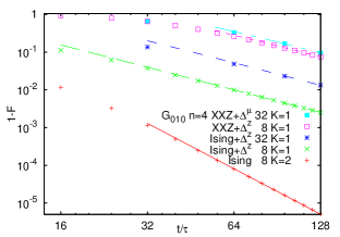
(b)
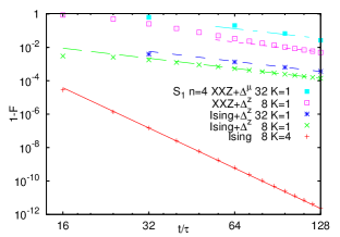
(c)

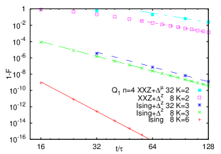
Figure 6: (color online) Illustration of decoupling accuracy with sequences 8 and 32 for chains of $n=4$ qubits with different couplings as indicated on the plots. The plots show average infidelity [see Eq. (59)] computed at fixed time $t$ as the pulse duration $\tau$ was reduced to accommodate a different number of sequences. The values of model parameters were randomly chosen and remained the same for all simulations. Symbols are the data points, lines are the single-parameter fits of the mismatch $\delta$ [see Eq. (58)] to $\delta=b\tau^{K}$, where the values of $K$ indicated on the plots correspond to those in Tab. 3. (a) Gaussian pulses; (b) 1st-order pulses $S_{1}$; (c) 2nd-order pulses $Q_{1}$.

We saw that with order-$K$ decoupling in multi-qubit systems with local couplings, the decoupling error operators can be represented as connected clusters of up to $K+1$ bonds. For a linear chain, these involve up to $K+2$ qubits, and the number of such operators scales linearly with the total number $n$ of qubits, as long as $n>K+2$. In an $n$-qubit system, each of such operators can be written as an outer product of the cluster contribution, and the identity operators for the remaining qubits. As a result, the square of the Frobenius norm of the error operators scales linearly with the size of the Hilbert space, that is, exponentially with the number of qubits. However, this exponential scaling is suppressed when we compute the infidelity [see Eq. (59)], so that the infidelity scales only linearly with the number of clusters, that is, linearly with the number of qubits. The same scaling with the system size is expected in higher dimensional arrangements of qubits (planar, 3D).

We illustrate the scaling of decoupling errors with the qubit number $n$ in Fig. 7. The plots show the scaling of the average infidelity at the end of the interval in Fig. 6 and other data with the chain length $n$.

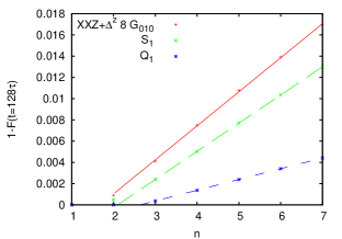
Figure 7: (color online) Scaling of the infidelity $1-F$ at $t/\tau=128$ with the chain length $n$ for a particular realization of an XXZ chain with on-site disorder $\Delta^{z}_{i}$, decoupling sequence 8, pulse shapes as indicated. (Data for the pulse $G_{010}$ divided by 10 to fit with the other data.) While the unitary matrix mismatch $\delta^{2}$ [see Eq. (58)] grows exponentially with the chain length $n$, $\delta^{2}\propto 2^{n}$, the leading-order contribution to the corresponding infidelity $(1-F)$ represents the probability of error in one of the clusters, and it scales only linearly, as also seen in the plots.

V.3 Composite pulses

Composite pulses are, in fact, pulse sequences designed to replace a single pulse and specially designed to compensate for some particular systematic errors, including off-resonance application, pulse amplitude, and pulse phase errorsZhang et al. (1990); Wimperis (1994); Cummins et al. (2003); Hugh and Twamley (2005); Brown et al. (2004b); Hedin and Furó (2002?); Schmidt-Kaler et al. (2003); Jones ; Mignon et al. (2004).

The off-resonance errors appear when the carrier frequency of the applied pulse is off the transition frequency between the $|0\rangle$ and $|1\rangle$ state of a qubit. In the rotating reference frame this is equivalent to a non-zero chemical shift Hamiltonian (3), with $\Delta$ equal to the corresponding frequency bias. We note that our 1st and 2nd-order self-refocusing pulse shapes already offer a degree of stability against such errors.

For this reason we concentrate on the pulse amplitude errors, where the correct pulse shape is applied with the wrong amplitude, producing an incorrect rotation angle $\tilde{\phi}_{0}\neq\phi_{0}$. Note that no one-dimensional pulse shaping can compensate for this kind of errors, since the modified rotation angle is simply proportional to the pulse amplitude, $\tilde{\phi}_{0}=(1+f)\phi_{0}$.

On the other hand, one can expect that the pulse amplitude offset $f$ remains the same for all the pulses applied at a particular frequency. This uniformity is utilized in several composite pulses designed so that the net rotation would be insensitive to such uniform errors.

V.3.1 SCROFULOUS

The three-pulse sequence SCROFULOUSCummins et al. (2003) is based on the sequence originally proposed by TyckoTycko (1983); Tycko et al. (1984). Particularly, an improved $\pi$ pulse is obtained by applying three $\pi$ pulses, at $60^{\circ}$, $300^{\circ}$, and again at $60^{\circ}$, or just $\pi_{60}\pi_{300}\pi_{60}$. In the case of ideal $\delta$-pulses, the resulting pulse compensates for pulse amplitude errors to linear order. With finite-width shaped pulses, an additional error is generated due to the presence of the system Hamiltonian. In particular, for the chemical-shift Hamiltonian (3), the expansion of a unitary operator applied along $x$ axis has the form [see Eqs. (42), (49)]

$$U_{x} = \cos\frac{\phi_{0}}{2}-i\sigma_{x}\sin\frac{\phi_{0}}{2}$$ (50)

$$-i{\tau\Delta\upsilon\over 2}\left(\cos\phi_{0}\sigma_{z}-\sigma_{y}\sin\phi_{0}\right)$$

$$+{\tau^{2}\Delta^{2}\upsilon^{2}\over 8}\left(i\sigma_{x}\sin\frac{\phi_{0}}{2}-\cos\frac{\phi_{0}}{2}\right)$$

$$+{\tau^{2}\Delta^{2}\alpha\over 4}\left(i\sigma_{x}\cos\frac{\phi_{0}}{2}+\sin\frac{\phi_{0}}{2}\right)+{\cal O}(\tau)^{3}.\quad$$

Combining the corresponding expressions appropriately rotated in the $x$-$y$ plane, and expanding the result to quadratic power in the relative amplitude offset $f$, we obtain for the composite pulse $\pi_{60}\pi_{300}\pi_{60}$,

$$U_{\mathrm{SCR}}=-i\sigma_{x}+i{\tau\Delta\tilde{\upsilon}}\sigma_{z}-{i}{\sqrt{3}\pi^{2}f^{2}\over 8}\sigma_{y}+\ldots,$$ (51)

where $\tilde{\upsilon}\equiv\tilde{\upsilon}(f)=\upsilon+\upsilon^{\prime}f+{\cal O}(f^{2})$ is the parameter $\upsilon$ [Eq. (40)] but for the pulse with rescaled amplitude, and the further terms are of order $f\tilde{\upsilon}\tau\Delta$, $\tilde{\upsilon}^{2}\tau^{2}\Delta^{2}$, $\tilde{\alpha}f\tau^{2}\Delta^{2}$. Clearly, with Gaussian or other pulse shape such that $\upsilon\neq 0$, the error is linear in $\tau\Delta$ and quadratic in the amplitude shift $f$ (although generally there will also be a cross-term $\propto f\tau\Delta$). This situation is illustrated in Fig. 8(a), where the average infidelity is plotted for the SCROFULOUS sequence with pulses $G_{010}$ on the plane $\Delta\tau$–$f$. The region for $1-F=10^{-5}$ is a narrow vertical line which corresponds to great sensitivity to frequency shift. With 1st-order self-refocusing pulses such that $\upsilon=0$, $\tilde{\upsilon}(f)\propto f$, the error is dominated by the term $\propto f\tau\Delta$. The corresponding region corresponds to a diamond-like shape in the center of Fig. 8(b). We have also generated self-refocusing pulse shapes such that both $\upsilon=0$ and $\upsilon^{\prime}=0$. Then, by symmetry, $\upsilon^{\prime\prime}=0$, and generically $\tilde{\upsilon}\propto f^{3}$. Then, for 1st-order pulses, $\alpha\neq 0$, the errors are dominated by the term omitted in Eq. (51); they scale as ${\cal O}(f^{2})$, ${\cal O}(\upsilon^{\prime\prime\prime}\Delta f^{3})$, ${\cal O}(\alpha\Delta^{2})$, while for second-order pulses the last two terms become ${\cal O}(\Delta^{3})$, ${\cal O}(\alpha^{\prime}f^{2}\Delta^{2})$. Plots for such shapes are shown in Figs. 8(c) and 8(d) respectively; the result of improved pulse stability is a much wider region of high fidelity.

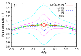
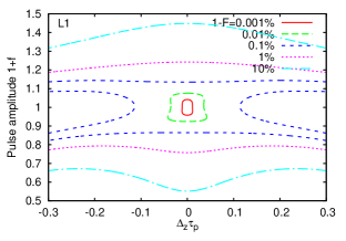
(a)
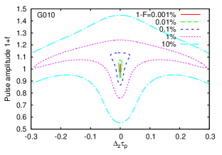
(b) (c) (c)

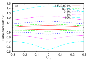
Figure 8: (color online) Contour plots of the average fidelity for the composite pulse SCROFULOUS $\pi_{60}\pi_{300}\pi_{60}$ with (a) Gaussian pulses $G_{010}$; (b) 1-st order self-refocusing pulses $S_{1}$ (the plots for pulses $Q_{1}$ look similarly but symmetric with respect to horizontal axis); (c) 1st-order pulse with amplitude correction $\upsilon=\upsilon^{\prime}=\upsilon^{\prime\prime}=0$; (d) 2nd-order pulse with amplitude correction, $\upsilon=\upsilon^{\prime}=\upsilon^{\prime\prime}=\alpha=0$. The axes are the relative frequency mismatch $\tau\Delta$ and the relative pulse amplitude $(1+f)$, see text.

V.3.2 BB₁ and related pulses

A longer but more accurate composite pulse known as BB₁ was originally proposed by WimperisWimperis (1994). For target angle $\theta=\pi$, the pulse can be written as BB${}_{1}^{(W)}=\pi_{0}\pi_{\phi}(2\pi)_{3\phi}\pi_{\phi}$, where $\phi=-\cos^{-1}(-1/4)\approx 104.5^{\circ}$. For ideal $\delta$-pulses, this cancels errors of both 1st and 2nd order in the relative pulse amplitude bias $f$. A related symmetrized sequence BB${}_{1}^{(CLJ)}=(\pi/2)_{0}\pi_{\phi}(2\pi)_{3\phi}\pi_{\phi}(\pi/2)_{0}$ was proposed in Ref. Cummins et al., 2003 [see also Ref. Hugh and Twamley, 2005]; because of the symmetry it leads to some additional error cancellation at higher order. With shaped pulses, we have also analyzed variants of these sequences with the $2\pi$ pulses replaced by two $\pi$ pulses, BB${}_{1}^{(W^{\prime})}=\pi_{0}\pi_{\phi}(\pi)_{3\phi}(\pi)_{3\phi}\pi_{\phi}$ and BB${}_{1}^{(CLJ^{\prime})}=(\pi/2)_{0}\pi_{\phi}(\pi)_{3\phi}(\pi)_{3\phi}\pi_{\phi}(\pi/2)_{0}$.

Computing the products of versions of Eq. (50) appropriately rotated in the $x$-$y$ plane, for on-resonance application of any version of the BB₁ sequence,

$$U_{{\rm BB}_{1}}^{(\Delta=0)}=-i\sigma_{x}-{f^{3}\pi^{3}\over 64}(5-i15^{1/2}\sigma_{z})+{\cal O}(f^{4}).$$ (52)

We note that to achieve the level of infidelity of, say, $1-F=10^{-4}$, the frequency mismatch should satisfy $|f|<0.136$, compared with $|f|<0.090$ for the SCROFULOUS sequence. Thus, even though order of the BB₁ family of composite pulses is higher (and thus, for small $|f|$ their performance is much better asymptotically), at this level of infidelity their performance is comparable.

We now turn to off-resonance correction terms which differ between implementations of the BB₁ sequence. In particular, with generic pulses such that $\upsilon\neq 0$, already at $f=0$, all of these sequences acquire linear corrections scaling with $\tau\Delta$. For example, the expansion of the sequence BB${}_{1}^{(W)}$ at $f=0$ can be written as

$$U_{{\rm BB}_{1}}^{(W,f=0)}=-i\sigma_{x}+i\frac{\tau\Delta}{2}\left(\sigma_{z}\upsilon_{1}-\sigma_{y}\upsilon_{2}\right)$$ (53)

$$+\frac{\tau^{2}\Delta^{2}}{16}\left(2i\sigma_{x}\upsilon^{2}+6\upsilon_{2}\upsilon_{1}+\alpha+i\sqrt{15}\sigma_{z}\left(\alpha-2\upsilon_{1}\upsilon_{2}\right)\right)$$

$$+{\cal O}(\Delta^{3}\tau^{3}),$$

where $\alpha\equiv 2\alpha_{1}-\alpha_{2}$, $\upsilon^{2}\equiv\upsilon_{1}^{2}+\upsilon_{2}^{2}$, and the parameters $\upsilon_{1}$, $\alpha_{1}$ and $\upsilon_{2}$, $\alpha_{2}$ correspond to the $\pi$ and $2\pi$ pulses respectively. Notice that the second-order coefficients $\alpha_{i}$ enter only in the combination $2\alpha_{1}-\alpha_{2}$. Not surprisingly, if we replace the $2\pi$-pulse with two $\pi$ pulses, the coefficients $\alpha$ cancel out,

$$U_{{\rm BB}_{1}}^{(W^{\prime},f=0)} = -i\sigma_{x}+i\frac{\tau\Delta\upsilon_{1}}{2}\sigma_{z}+i\frac{\tau^{2}\Delta^{2}\upsilon_{1}^{2}}{8}\sigma_{x};$$ (54)

thus second-order accuracy can be obtained already with 1st order pulses, $\upsilon_{1}=0$. Now, when both the amplitude and the resonant frequency bias are present, $f\neq 0$ and $\Delta\neq 0$, there is an additional source of error due to dependence of the pulse parameters on the amplitude, $\upsilon,\alpha\to\tilde{\upsilon}(f),\tilde{\alpha}(f)$. For regular self-refocusing pulses, $\tilde{\upsilon}(f)=\upsilon^{\prime}f+{\cal O}(f^{2})$, and the 1st order terms in Eqs. (53), (54) and their analogs for the other variants of the BB₁ pulse dominate the error $\propto f\tau\Delta$. Respectively, the average infidelity scales as $\propto(f\tau\Delta)^{2}$, resulting in characteristic diamond-like shape on the contour plots of infidelity, see Figs. 9(a,b), 10(a).

With specially designed pulses such that both $\upsilon=0$ and $\upsilon^{\prime}=0$, due to pulse symmetry, also $\upsilon^{\prime\prime}=0$, so that $\upsilon(f)=\upsilon^{\prime\prime\prime}f^{3}+{\cal O}(f^{4})$. Then, for sequences other than BB${}_{1}^{(W^{\prime})}$, with 1st-order pulses the error is dominated by the terms quadratic in $\tau\Delta$ due to coefficients $\alpha_{i}$ [cf. Eq. (53)]. As a result, the high-fidelity regions in Figs. 9(c), 10(b), and 11(a) have much more rounded shape. With 2nd-order pulses with amplitude correction, such that $\alpha_{i}=0$ but $\alpha_{i}^{\prime}\neq 0$, the leading-order error scales as ${\cal O}(f\tau^{2}\Delta^{2})$, which extends the high-fidelity regions out to larger values of $\tau\Delta$ in a characteristic “smile” pattern. For the sequence BB${}_{1}^{(W^{\prime})}$ these terms cancel out, and the leading-order error term comes from the non-zero $\upsilon^{\prime\prime\prime}$, the errors scale as $\propto f^{3}\tau\Delta$,

$$U_{{\rm BB}_{1}}^{(W^{\prime})}=U_{{\rm BB}_{1}}^{(W^{\prime},f=0)}+i{f^{3}\tau\Delta\,\upsilon_{1}^{\prime\prime\prime}\over 2}\sigma_{z}+{\cal O}(\tau^{3}\Delta^{3}).$$ (55)

This error has the same order in $f$ as that in Eq. (52), and it can compensate or increase the contribution linear in $\sigma_{z}$. The result is a somewhat skewed in the center high-fidelity region widely stretched horizontally.

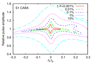
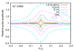
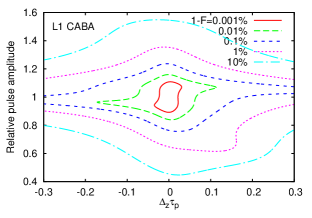
(a) (b) (c) (d)

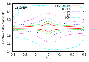
Figure 9: (color online) Contour plots of the average infidelity $1-F$ for the composite pulse BB${}_{1}^{(W)}$ [$\pi_{0}\pi_{\phi}(2\pi)_{3\phi}\pi_{\phi}$] with (a) 1st-order self-refocusing pulses $S_{1}$; (b) 2nd-order pulses $Q_{1}$; (c) 1st-order pulses with amplitude correction; (d) 2nd-order pulses with amplitude correction. The axes are the relative frequency mismatch $\tau\Delta$ and the relative pulse amplitude $(1+f)$, see text.

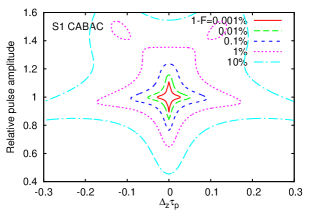
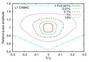
(a) (b) (c)

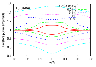
Figure 10: (color online) As in Fig. 9 but for the symmetrized sequence BB${}_{1}^{(CLJ)}$ [$(\pi/2)_{0}\pi_{\phi}(2\pi)_{3\phi}\pi_{\phi}(\pi/2)_{0}$]. The pulse shapes are (a) 1st-order pulses $S_{1}$ (the fidelity for the 2nd-order pulses $Q_{1}$ is similar); (b) 1st-order pulses with amplitude correction; (c) 2nd-order pulses with amplitude correction. Note how regular are the shapes of high-fidelity regions.

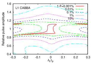
(a) (b)

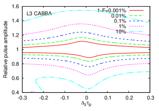
Figure 11: (color online) As in Fig. 9 but for the sequence BB${}_{1}^{W^{\prime}}$ [$\pi_{0}\pi_{\phi}\pi_{3\phi}\pi_{3\phi}\pi_{\phi}$] using only $\pi$-pulses. (a) 1st-order pulses with amplitude correction; (b) 2nd-order pulses with amplitude correction. The absence of the error terms linear in $\alpha$ [see Eqs. (54), (55)] produces a much wider high-fidelity region already with 1st-order pulses.

V.4 Stability of decoupling against amplitude errors

We now return to the problem of decoupling for a chain of qubits, but now consider the effect of the amplitude errors. This needs a separate study since single-qubit errors with composite pulses have structure different from those due to, say, finite pulse width.

In Fig. 12(a) we present the results of simulations for a particular 4-qubit Ising chain with on-site chemical potential shifts $\Delta^{z}_{i}$ over time interval $t=128\tau$ (exactly the same parameters as in Figs. 6, 7). Specifically, we plot the infidelity $(1-F)$ in units of $10^{-4}$, as a function of the fractional pulse amplitude $1+f$. In the first half of the symmetric sequence $\textbf{8}={\rm X}_{1}{\rm Y}_{2}\bar{\rm X}_{1}\bar{Y}_{2}\,\bar{Y}_{2}\bar{\rm X}_{1}{\rm Y}_{2}{\rm X}_{1}$, we used the original BB${}_{1}^{(W)}$ pulse ${\rm X}\to\pi_{0}\pi_{\phi}(2\pi)_{3\phi}\pi_{\phi}$ for $\pi_{x}$, rotated appropriately to implement ${\rm Y}\to\pi_{\pi/2}\pi_{\phi+\pi/2}(2\pi)_{3\phi+\pi/2}\pi_{\phi+\pi/2}$ as well as $\bar{\rm X}\equiv{\rm X}_{\pi}$, while in the second part of the sequence we used the same decomposition but backwards, e.g., ${\rm X}\to\pi_{\phi}(2\pi)_{3\phi}\pi_{\phi}\pi_{0}$. Here $\phi=-\cos^{-1}(-1/4)\approx 104.5^{\circ}$. With no amplitude mismatch, thus constructed decoupling sequence has order $K=1$ with 1st-order pulses, and an almost-2nd order “$1$*” with 2nd-order pulses, with the norm of the 2nd-order term reduced by three orders of magnitude compared to 1st-order pulses. These should be compared with $K=1$ and $K=3$ respectively for the regular 8-pulse sequence [Tab. 3].

It is seen from Fig. 12(a) that regular 1st- and 2nd-order pulses $S_{1}$ and $Q_{1}$ perform in the BB₁-corrected composite sequence almost as well as the self-refocusing pulses with additional amplitude protection (1st-order $L_{1}$ and 2nd-order $L_{3}$). In addition, the 2nd-order pulses with amplitude protection ($L_{3}$) work almost as well in the regular 8-pulse sequence. All of these allow to achieve the infidelity level of $10^{-4}$ at amplitude mismatch of $3\%$ or higher (up to $6\%$ with pulses $L_{3}$ in the sequence 8BB₁). With the regular 8-pulse sequence, the region of high fidelity shrinks substantially for pulses $Q_{1}$ and $L_{1}$, and it all but disappears for the pulse S₁ [the coefficient $\alpha$ for the pulse $L_{1}$ happens to be a few times smaller than that for $S_{1}$].

The results of analogous calculation for a particular 4-qubit XXZ chain with on-site chemical potential shifts $\Delta^{z}_{i}$ over time interval $t=128\tau$ (exactly the same parameters as in Figs. 6, 7) are presented in Fig. 12(b). However, it turns out that the BB₁ composite pulses lose accuracy when used with XXZ chain. Even in the absence of amplitude errors, there are linear errors in $\tau J^{\perp}$ [the zeroth order average Hamiltonian is non-zero]. Thus, we only present the results for the regular 8-pulse sequence. With this sequence, the decoupling orders for 1st- and 2nd-order pulses are $K=1$ and $K=2$ respectively [Tab. 3]. Compared with Ising-only couplings, with the particular parameters chosen, this increases the infidelity by some five orders of magnitude with pulses Q₁ [Fig. 6(c)], and by some two orders of magnitude for pulses $S_{1}$ [Fig. 6(b)]. As for the Ising chain, the effect of the amplitude errors is weaker with specially-designed pulses $L_{1}$ and $L_{3}$ such that the 1st-order coefficient $\tilde{\upsilon}(f)$ scales as a higher power of $f$. With the pulse $L_{1}$, the 2nd-order coefficient $\alpha$ is non-zero but small; it is seen from Fig. 12(b) that its effect is to introduce a linear term $1-F\propto f$ which tends to skew the infidelity minimum away from $f=0$. We should also note that with the Gaussian pulses G₀₁₀ (not shown), even the on-resonance infidelity is out of range of the plots Fig. 12.

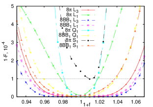
(a) (b)

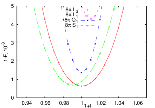
Figure 12: (color online) Decoupling errors as a function of relative pulse amplitude for a chain of $n=4$ qubits with different decoupling schemes as indicated. (a) Ising chain in the presence of individual chemical shifts $\Delta^{z}_{i}$. 8-pulse sequence with BB₁ composite pulses offers the best accuracy, which remains essentially the same whether the sequence is used with regular 1st- or 2nd- order pulses or with the pulses stabilized against amplitude errors (1st-order pulses $L_{1}$ and 2nd-order pulses $L_{3}$). However, the pulse $L_{3}$ works well enough even with regular 8-pulse sequence. While the details of the amplitude scaling differ, at the level of $1-F=10^{-4}$, the 1st-order amplitude-protected pulses $L_{1}$ and regular 2nd-order pulses $Q_{1}$ have comparable accuracy. The use of 1st-order pulses show relatively poor performance even on resonance. (b) XXZ chain in the presence of individual chemical shifts $\Delta^{z}_{i}$. With XXZ coupling, The BB₁ composite pulse is no longer accurate, as the errors appear already in the linear order in $\tau J^{\perp}$ (not shown). With the regular 8-pulse sequence 8, the best accuracy is obtained for the pulses with amplitude correction.

VI Conclusions

We presented a comprehensive study targeting pulse and sequence design and analysis based on a consistent high-order average Hamiltonian expansion. The numerical technique for expanding the evolution operator was originally introduced by us in Ref. Sengupta and Pryadko, 2005, and a complimentary analytical technique was developed for $\pi$-pulses by one of the authors in Ref. Pryadko and Quiroz, 2007.

The overall approach is to start with a closed system described by a finite-dimensional Hamiltonian $H_{S}$ and design a sequence of shaped pulses such that the evolution operator would be accurate to a given order $K$ in powers of $H_{S}$. The key to this approach are the NMR-style 1st- and 2nd-order self-refocusing one-dimensional pulses constructed for a single-qubit chemical-shift Hamiltonian (3). In this work we designed a number of such shapes for different rotation angles $\phi_{0}$, and presented a careful analytical analysis of the first two leading orders of the average Hamiltonian theory for driven qubit evolution with the most general system Hamiltonian $H_{S}$. While any symmetric one-dimensional pulse shape is characterized by only three parameters, two of these can be set to zero by pulse shaping. The remaining parameter is also non-zero for an ideal “hard” $\delta$-function pulse. This leads to an important conclusion that the constructed pulses can be used as drop-in replacement for hard pulses; with proper pulse placement the results should be identical to first two orders. The structure of errors appearing in higher orders of the evolution operator can be understood by analyzing the numerical time-dependent perturbation series for the evolution operator of a closed system.

An important advantage of this approach is that the expansion order offers a natural classification of the error operators. As a result, (i) the convergence regions have regular shapes as a function of parameters [see Figs. 10(c,d) and 11(b,c)]. Furthermore, with local two- (or few-)qubit couplings dominant, (ii) the error operators can be placed on connected clusters of up to $k+1$ qubits for terms of order $k$, which allows one to understand their structure in terms, e.g., the direct products of up to $(k+1)$ Pauli matrices. Once their structure understood, the convergence can be readily improved by suppressing the error operators, as in our analysis of pulse-amplitude errors. We emphasize, that such an analysis can be performed even for very large qubit systems. Thus, (iii) this approach is characterized by scalability with the system size, as we illustrated by analyzing decoupling infidelity with the system size [Fig. 7]. Although in this work we concentrated on the dynamics of closed systems, another important advantage is that (iv) the high-order control sequences result in lower decoherence in the presence of slow environmental modesPryadko and Sengupta (2006); Pryadko and Quiroz (2007).

Most obvious application of highly-optimized shaped pulses of the sort presented in this work is in solid-state quantum computation, where the bandwidth available for quantum gates is typically limited. Our techniques based on analytical and numerical high-order average Hamiltonian theory offers a systematic scalable approach for constructing gates for such multi-qubit systems, without need of solving their full dynamics. However, even if the bandwidth does not appear to be at premium, simple pulse shaping (e.g., using 1st-order pulses) can still offer a substantial improvement of control accuracy.

VII Acknowledgments.

This research was supported in part by the NSF grant No. 0622242 (LP). LANL is supported by US DOE under Contract No. W-7405-ENG-36. NHMFL is supported by the DOE, the NSF, and the state of Florida.

Appendix A Average fidelity

Here we discuss the calculation of the fidelity averaged over the initial state, in the case of unitary evolution with known evolution matrix $U$, while the desired evolution matrix is $U_{0}$. Let us write the density matrix of the initial pure state as $\rho_{0}=\psi\psi^{\dagger}$, where $\psi$ is an $N$-component complex vector. Then the actual density matrix is $\rho=U\psi\psi^{\dagger}U^{\dagger}$, while the desired density matrix is $\rho_{\mathrm{ideal}}=U_{0}\psi\psi^{\dagger}U_{0}^{\dagger}$. The fidelity with the given initial state

$$F_{\psi} \equiv \mathop{\rm tr}(\rho_{\mathrm{ideal}}\rho)=\mathop{\rm tr}(U_{0}\psi\psi^{\dagger}U_{0}^{\dagger}U\psi\psi^{\dagger}U^{\dagger})$$ (56)

$$= \sum_{ijkl}\psi_{i}\psi_{j}^{*}(U_{0}^{\dagger}U)_{ik}\psi_{k}\psi^{*}_{l}(U_{0}^{\dagger}U)^{*}_{jl}.$$

The only condition on the components $\psi_{i}$ of the wavefunction is the normalization, $1=\psi^{\dagger}\psi=\sum_{i}|\psi_{i}|^{2}$. Generally, this means that the average of the product in Eq. (56) can only depend on the identity tensor $\delta_{ij}$. By symmetry, $\langle\psi_{i}\psi_{j}^{*}\psi_{k}\psi^{*}_{l}\rangle=A(\delta_{ij}\delta_{kl}+\delta_{il}\delta_{kj})$, where the unknown coefficient $A$ can be computed from the normalization by tracing over $i=j$, $k=l$. We obtain $1=A(N^{2}+N)$, so that the average fidelity

$$F={N+|\mathop{\rm tr}V|^{2}\over N+N^{2}},\quad 1-F={N^{2}-|\mathop{\rm tr}V|^{2}\over N+N^{2}},$$ (57)

where $V\equiv U_{0}^{\dagger}U$. Numerically, with $V$ close to identity matrix, the loss of precision can be avoided by expressing the infidelity $1-F$ in terms of the modified mismatch,

$$\delta^{2}=\mathop{\rm tr}(\openone-\tilde{V})^{\dagger}(\openone-\tilde{V}),\quad\tilde{V}=V{|\mathop{\rm tr}V|\over\mathop{\rm tr}V}.$$ (58)

Namely, since $\delta^{2}=2N-2|\mathop{\rm tr}V|$, the average infidelity can be written as

$$1-F={\delta^{2}(4N-\delta^{2})\over 4(N+N^{2})}.$$ (59)

References

- Vandersypen et al. (2001) L. M. K. Vandersypen, M. Steffen, G. Breyta, C. S. Yannoni, M. H. Sherwood, and I. L. Chuang, Nature 414, 883 (2001).
- Leskowitz et al. (2003) G. M. Leskowitz, N. Ghaderi, R. A. Olsen, and L. J. Muller, J. Chem. Phys. 119, 1643 (2003).
- Yannoni et al. (1999) C. S. Yannoni, M. H. Sherwood, D. C. Miller, I. L. Chuang, L. M. K. Vandersypen, and M. G. Kubinec, App. Phys. Lett. 75, 3563 (1999).
- Vandersypen and Chuang (2004) L. M. K. Vandersypen and I. L. Chuang, Reviews of Modern Physics 76, 1037 (2004).
- Slichter (1992) C. P. Slichter, Principles of Magnetic Resonance (Springer-Verlag, New York, 1992), 3rd ed.
- Knill et al. (1998) E. Knill, R. Laflamme, and W. H. Zurek, Science 279, 342 (1998).
- Fowler et al. (2004) A. G. Fowler, C. D. Hill, and L. C. L. Hollenberg, Phys. Rev. A 69, 042314 (2004).
- Price et al. (2000) M. D. Price, T. F. Havel, and D. G. Cory, New J. Phys. 2, 10 (2000).
- Boulant et al. (2003) N. Boulant, K. Edmonds, J. Yang, M. A. Pravia, and D. G. Cory, Phys. Rev. A 68, 032305 (2003).
- Sanders et al. (1999) G. D. Sanders, K. W. Kim, and W. C. Holton, Phys. Rev. A 59, 1098 (1999).
- Hodgkinson et al. (2000) P. Hodgkinson, D. Sakellariou, and L. Emsley, Chem. Phys. Lett. (2000).
- Niskanen et al. (2003) A. O. Niskanen, J. J. Vartiainen, and M. M. Salomaa, Phys. Rev. Lett. 90, 197901 (2003).
- Steffen and Koch (2007) M. Steffen and R. H. Koch, Phys. Rev. A 75, 062326 (2007).
- Warren (1984) W. S. Warren, J. Chem. Phys. 81, 5437 (1984).
- Bauer et al. (1984) C. Bauer, R. Freeman, T. Frenkiel, J. Keeler, and A. J. Shaka, J. Mag. Res. 58, 442 (1984).
- Geen and Freeman (1991) H. Geen and R. Freeman, J. Mag. Res. 93, 93 (1991).
- Goswami (2003) D. Goswami, Phys. Rep. 374, 385 (2003).
- Sengupta and Pryadko (2005) P. Sengupta and L. P. Pryadko, Phys. Rev. Lett. 95, 037202 (2005).
- Freeman (1998) R. Freeman, Progr. NMR Spectr. 32, 59 (1998).
- Pryadko and Quiroz (2007) L. P. Pryadko and G. Quiroz, Phys. Rev. A 77, 012330/1 (2007).
- Hahn (1950) E. L. Hahn, Phys. Rev. 80, 580 (1950).
- Steffen et al. (2003) M. Steffen, J. M. Martinis, and I. L. Chuang, Phys. Rev. B 68 (2003).
- Chen et al. (2001) P. Chen, C. Piermarocchi, and L. J. Sham, Phys. Rev. Lett. 87, 067401 (2001).
- Mehring (1983) M. Mehring, Principles of high-resolution NMR in solids (Springer-Verlag, New York, 1983).
- Waugh et al. (1968a) J. S. Waugh, L. M. Huber, and U. Haeberlen, Phys. Rev. Lett. 20, 180 (1968a).
- Waugh et al. (1968b) J. S. Waugh, C. H. Wang, L. M. Huber, and R. L. Vold, J. Chem. Phys. 48, 652 (1968b).
- Domb and Green (1974) C. Domb and M. S. Green, eds., Phase transitions and critical phenomena, vol. 3 (Academic, London, 1974).
- G. A. Baker (1990) J. G. A. Baker, Quantitative theory of critical phenomena (Academic, San Diego, 1990).
- Galassi et al. (2003) M. Galassi, J. Davies, J. Theiler, B. Gough, G. Jungman, M. Booth, and F. Rossiet, GNU Scientific Library Reference Manual, 2nd ed. (2003), Network Theory Ltd., http://www.gnu.org/software/gsl/.
- Pryadko and Sengupta (2006) L. P. Pryadko and P. Sengupta, Phys. Rev. B 73, 085321 (2006).
- Kofman and Kurizki (2001) A. G. Kofman and G. Kurizki, Phys. Rev. Lett. 87, 270405 (2001).
- Kofman and Kurizki (2004) A. G. Kofman and G. Kurizki, Phys. Rev. Lett. 93, 130406 (2004).
- Facchi et al. (2005) P. Facchi, S. Tasaki, S. Pascazio, H. Nakazato, A. Tokuse, and D. A. Lidar, Phys. Rev. A 71, 022302 (2005).
- Brown et al. (2004a) K. R. Brown, A. W. Harrow, and I. L. Chuang, Phys. Rev. A 70, 052318 (2004a).
- Khodjasteh and Lidar (2005) K. Khodjasteh and D. A. Lidar, Phys. Rev. Lett. 95, 180501 (2005).
- Zhang et al. (1990) S. Zhang, X. Wu, and M. Mehring, Chem. Phys. Lett. 173, 481 (1990).
- Wimperis (1994) S. Wimperis, J. Magn. Res., Ser. A 109, 221 (1994).
- Cummins et al. (2003) H. K. Cummins, G. Llewellyn, and J. A. Jones, Phys. Rev. A 67, 042308 (2003).
- Hugh and Twamley (2005) D. M. Hugh and J. Twamley, Phys. Rev. A 71, 012327 (2005).
- Brown et al. (2004b) K. R. Brown, A. W. Harrow, and I. L. Chuang, Phys. Rev. A 70, 052318 (2004b).
- Hedin and Furó (2002?) N. Hedin and I. Furó, JMRE p. ? (2002?).
- Schmidt-Kaler et al. (2003) F. Schmidt-Kaler, H. Häffner, M. Riebe, S. Gulde, G. P. T. Lancaster, T. Deuschle, C. Becher, C. F. Roos, J. Eschner, and R. Blatt, Letters to Nature 422, 408 (2003).
- (43) J. A. Jones, arXiv:quant-ph/0301019v1, http://arxiv.org/abs/quant-ph/0301019.
- Mignon et al. (2004) C. Mignon, Y. Millot, and P. P. Man, C. R. Chimie 7, 425 (2004).
- Tycko (1983) R. Tycko, Phys. Rev. Lett. 51, 775 (1983).
- Tycko et al. (1984) R. Tycko, H. M. Cho, E. Schneider, and A. Pines, J. Magn. Reson. (1984).