On the Capacity Equivalence with Side Information at Transmitter and Receiver

Abstract

In this paper, a channel that is contaminated by two independent Gaussian noises $S\sim\mathcal{N}(0,Q)$ and ${Z_{0}}\sim\mathcal{N}(0,N_{0})$ is considered. The capacity of this channel is computed when independent noisy versions of ${S}$ are known to the transmitter and/or receiver. It is shown that the channel capacity is greater then the capacity when ${S}$ is completely unknown, but is less then the capacity when ${S}$ is perfectly known at the transmitter or receiver. For example, if there is one noisy version of ${S}$ known at the transmitter only, the capacity is $\frac{1}{2}\log(1+\frac{P}{Q(N_{1}/(Q+N_{1}))+N_{0}})$, where $P$ is the input power constraint and $N_{1}$ is the power of the noise corrupting $S$. Further, it is shown that the capacity with knowledge of any independent noisy versions of $S$ at the transmitter is equal to the capacity with knowledge of the statistically equivalent noisy versions of $S$ at the receiver.

I INTRODUCTION

Consider a channel in which the received signal, $\mathbf{Y}$ is corrupted by two independent additive white Gaussian noise (AWGN) sequences, $\mathbf{S}\sim\mathcal{N}(0,Q\mathbf{I}_{n})$ and $\mathbf{Z}_{0}\sim\mathcal{N}(0,N_{0}\mathbf{I}_{n})$, where $\mathbf{I}_{n}$ is the identity matrix of size $n$. The received signal is of the form,

$$\mathbf{Y}=\mathbf{X}+\mathbf{S}+\mathbf{Z}_{0},$$ (1)

where $\mathbf{X}$ is the transmitted sequence for $n$ uses of the channel. Let the transmitter and receiver each has knowledge of independent noisy observations of one of the noises, $\mathbf{S}$. We quantify the benefit of this additional knowledge by computing the capacity of the channel in (1) and presenting the coding scheme that achieves capacity. Our result indicates that the capacity is of the form $\frac{1}{2}\log(1+\frac{P}{\mu Q+N_{0}})$, where $0\leq\mu\leq 1$ is the residual fraction (explicitly characterized in Section II) of the interference power, $Q$, that can not be canceled with the noisy observations at the transmitter and receiver.

One special case of our model is when a noisy version of $\mathbf{S}$ is known only to the transmitter; our result in this case is a generalization of Costa’s celebrated result [1]. In [1], it is shown that the achievable rate when the noise $\mathbf{S}$ is perfectly known at the transmitter is equivalent to the rate when $\mathbf{S}$ is known at the receiver, and this rate does not depend on the variance of $\mathbf{S}$. A new coding strategy to achieve this capacity was also introduced in [1] and is popularly referred to as dirty paper coding (DPC). We generalize Costa’s result to the case of noisy interference knowledge. We show that the capacity with knowledge of a noisy version of $\mathbf{S}$ at the transmitter is equal to the capacity with knowledge of a statistically equivalent noisy version of $\mathbf{S}$ at the receiver. However, unlike [1] where the capacity does not depend on the variance of $\mathbf{S}$, in the general noisy side information case, the capacity decreases as the variance of $\mathbf{S}$ increases.

We also compute the capacity when multiple independent noisy observations of $\mathbf{S}$ are available at the transmitter and receiver. We show that in this case, it is sufficient for the transmitter and receiver to each compute maximum-likelihood estimates of $\mathbf{S}$ based on their observations and then use these estimates to achieve capacity using the coding strategy proposed in Section II-C. Further, it is shown that the capacity of a Gaussian channel with multiple independent observations of $\mathbf{S}$ known at the transmitter is equal to the capacity with statistically similar observations known at the receiver.

The proposed model can have several potential applications. For instance, consider the following scenario. Node A is transmitting to node B, but whose signal is also received at nodes C and D who are communicating with each other. Thus, nodes C and D can use the noisy estimate of user A’s signal to improve the rate at which they communicate.

In [1], Costa adopted the random coding argument given by Gel’fand and Pinsker [2] and El Gamal and Heegard [3]. In [2], the capacity of a discrete memoryless channel with side information at the encoder is derived and the result has been extended to the case when each of the encoder and decoder has one of two correlated side information [4]. Based on the channel capacity $C=\max_{p(u,x|s)}\{I(U;Y)-I(U,S)\}$ given in [2, 3], Costa constructed the auxiliary variable ${U}$ as a linear combination of ${X}\sim\mathcal{N}(0,P)$ and ${S}\sim\mathcal{N}(0,Q)$ and showed that this simple construction of ${U}$ achieves capacity. In our proof for achievability, we also follow the arguments from [2, 3]. Further, similar to [1], the optimal auxiliary variable in our case is also a linear combination of ${X}$ and the noisy observations of ${S}$ at the encoder. Thus, our coding scheme can be viewed as a variation of DPC.

Following the pioneering work of Costa, several extensions of DPC have been studied, e.g., colored Gaussian noise [5], arbitrary distributions of $\mathbf{S}$ [6] and deterministic sequences [7]. In [8], DPC has been applied to the AWGN and jitter channel and the rate loss due to imperfect synchronization at the decoder has been evaluated. DPC has also been extensively applied to watermarking or information embedding [9, 10] applications and for the Gaussian broadcast channel [11, 12]. In [13] the authors consider the case when $\mathbf{S}$ is perfectly known to the encoder and a noisy version is known to the decoder. Most of the analysis in [13] is for discrete memoryless channels and also causal knowledge of interference. The only result in [13] for Gaussian channel shows that there is no additional gain due to the presence of the noisy estimate at the decoder, since perfect knowledge is available at the encoder and a DPC can be constructed. In contrast, in this paper we study the case when only noisy knowledge of $\mathbf{S}$ is available at both transmitter and receiver.

Throughout this paper we only consider the case of non-causal knowledge of the interference. Causal extensions to these should be studied in future work. The rest of this paper is organized as follows: Section II introduces the system model and also gives the main capacity result. Extensions of the result to single and multiple noisy observations are evaluated in Section III. Brief concluding remarks are given in Section IV.

II SYSTEM MODEL, CAPACITY and ACHIEVABILITY

In this section, we first introduce the channel model and then compute the capacity of this channel.

II-A Channel Model

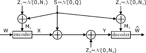
Figure 1: Channel model.

The channel model is depicted in Fig. 1. The communication problem is to send an index, $W\in\{1,2,\ldots,K\}$, to the receiver in $n$ uses of the channel. The transmission rate is $R=\frac{1}{n}\log_{2}K$ bits per transmission. The output of the channel is given in (1) and is contaminated by two independent AWGN sequences, $\mathbf{S}\sim\mathcal{N}(0,Q\mathbf{I}_{n})$ and $\mathbf{Z}_{0}\sim\mathcal{N}(0,N_{0}\mathbf{I}_{n})$. Side information $\mathbf{M}_{1}=\mathbf{S}+\mathbf{Z}_{1}$, which is noisy observations of the interference is assumed to be available at the transmitter for all $n$ uses of the channel. Similarly, noisy side information $\mathbf{M}_{2}=\mathbf{S}+\mathbf{Z}_{2}$, is assumed to be available at the receiver for all $n$ uses of the channel. The noise vectors are distributed as $\mathbf{Z}_{1}\sim\mathcal{N}(0,N_{1}\mathbf{I}_{n})$ and $\mathbf{Z}_{2}\sim\mathcal{N}(0,N_{2}\mathbf{I}_{n})$.

Based on the index $W$ and the observation $\mathbf{M_{1}}$, the encoder transmits one codeword, $\mathbf{X}$, from a $(2^{nR},n)$ code book. The codeword $\mathbf{X}$ must satisfy an average power constraint of the form, $\frac{1}{n}\|\mathbf{X}\|^{2}\leq P$. Let $\hat{W}$ be the estimate at the receiver of the transmitted index; an error occurs if $\hat{W}\neq W$.

II-B Channel Capacity

Theorem 1

Consider a channel of the form (1) with an average transmit power constraint $P$. Let independent noisy observations $\mathbf{M}_{1}=\mathbf{S}+\mathbf{Z}_{1}$ and $\mathbf{M}_{2}=\mathbf{S}+\mathbf{Z}_{2}$ of the interference $\mathbf{S}$ be available, respectively, at the transmitter and receiver. The noise vectors have the following distributions: $\mathbf{Z}_{i}\sim\mathcal{N}(0,N_{i}\mathbf{I}_{n})$, $i=0,1,2$ and $\mathbf{S}\sim\mathcal{N}(0,Q\mathbf{I}_{n})$. The capacity of this channel equals $\frac{1}{2}\log\left(1+\frac{P}{\mu Q+N_{0}}\right)$, where $0\leq\mu=\frac{1}{1+\frac{Q}{N_{1}}+\frac{Q}{N_{2}}}\leq 1$.

Remark: It is clear that $\mu=0$ when either $N_{1}=0$ or $N_{2}=0$. Consequently, the capacity is $\frac{1}{2}\log\left(1+\frac{P}{N_{0}}\right)$, which is consistent with the result in [1]. Further, $\mu=1$ when $N_{1}\rightarrow\infty$ and $N_{2}\rightarrow\infty$, and the capacity is $\frac{1}{2}\log\left(1+\frac{P}{Q+N_{0}}\right)$, which is the capacity of a Gaussian channel with noise variance $Q+N_{0}$. Thus, one can interpret $\mu$ as the residual fractional power of the interference that cannot be canceled by the noisy observations at the transmitter and receiver.

Proof: We first compute an outer bound on the capacity of this channel. It is clear that the channel capacity can not exceed $\max_{p(x|m_{1},m_{2})}I(X;Y|M_{1},M_{2})$, which is the capacity when both $M_{1}$ and $M_{2}$ are known at the transmitter and receiver. Thus, a capacity bound of the channel can be calculated as

$$~{}I(X;Y|M_{1},M_{2})=I(X;Y,M_{1},M_{2})-I(X;M_{1},M_{2})$$

$$\leq ~{}I(X;Y,M_{1},M_{2})$$ (2)

$$= ~{}H(X)+H(Y,M_{1},M_{2})-H(X,Y,M_{1},M_{2})$$

$$= ~{}{\frac{1}{2}\log(2\pi e)^{4}P\left|\begin{array}[]{ccc}P+Q+N_{0}&Q&Q\\ Q&Q+N_{1}&Q\\ Q&Q&Q+N_{2}\end{array}\right|}$$ (6)

$$~{}-{\frac{1}{2}\log(2\pi e)^{4}\left|\begin{array}[]{cccc}P&P&0&0\\ P&P+Q+N_{0}&Q&Q\\ 0&Q&Q+N_{1}&Q\\ 0&Q&Q&Q+N_{2}\\ \end{array}\right|}$$ (11)

$$= ~{}\frac{1}{2}\log\left(1+\frac{P}{\mu Q+N_{0}}\right).$$ (12)

where $\mu=\frac{1}{1+\frac{Q}{N_{1}}+\frac{Q}{N_{2}}}$. Note that the inequality in (2) is actually a strict equality since $I(X;M_{1},M_{2})=0$.

II-C Achievability of Capacity

We now prove that the capacity computed in (12) is achievable. The codebook generation and encoding method we use follows the principles introduced in [2, 3]. The construction of auxiliary variable is similar to [1].

Random codebook generation:

1. Generate $2^{nI(U;Y,M_{2})}$ i.i.d. length-$n$ codewords $\mathbf{U}$, whose elements are drawn i.i.d. according to $U\sim\mathcal{N}(0,P+\alpha^{2}(Q+N_{1}))$, where $\alpha$ is a coefficient to be optimized.

2. Randomly place the $2^{nI(U;Y,M_{2})}$ codewords $\mathbf{U}$ into $2^{nR}$ cells in such a way that each of the cells has the same number of codewords. The codewords and their assignments to the $2^{nR}$ cells are revealed to both the transmitter and the receiver.

Encoding:

1. Given an index $W$ and an observation, $\mathbf{M_{1}}=\mathbf{M_{1}}(i)$, of the Gaussian noise sequence, $\mathbf{S}$, the encoder searches among all the codewords $\mathbf{U}$ in the $W^{th}$ cell to find a codeword that is jointly typical with $\mathbf{M_{1}}(i)$. According to the joint asymptotic equipartition property (AEP) [14], it is easy to show that if the number of codewords in each cell is larger than or equal to $2^{nI(U,M_{1})}$, the probability of finding such a codeword $\mathbf{U}=\mathbf{U}(i)$ exponentially approaches $1$ as $n\rightarrow\infty$.

2. Once a jointly typical pair $(\mathbf{U}(i),\mathbf{M_{1}}(i))$ is found, the encoder calculates the codeword to be transmitted as $\mathbf{X}(i)=\mathbf{U}(i)-\alpha\mathbf{M_{1}}(i)$. With high probability, $\mathbf{X}(i)$ will be a typical sequence which satisfies $\frac{1}{n}\|\mathbf{X}(i)\|^{2}\leq P$.

Decoding:

1. Given $\mathbf{X}(i)$ is transmitted, the received signal is $\mathbf{Y}(i)=\mathbf{X}(i)+\mathbf{S}+\mathbf{Z_{0}}$. The decoder searches among all $2^{nI(U;Y,M_{2})}$ codewords $\mathbf{U}$ for a sequence that is jointly typical with $\mathbf{Y}(i)$. By joint AEP, the decoder will find $\mathbf{U}(i)$ as the only jointly typical codeword with probability approaching 1.

2. Based on the knowledge of the codeword assignment to the cells, the decoder estimates $\hat{W}$ as the index of the cell that $\mathbf{U}(i)$ belongs to.

Proof of achievability:

Let $U=X+\alpha M_{1}=X+\alpha(S+Z_{1})$, $Y=X+S+Z_{0}$ and $M_{2}=S+Z_{2}$, where $X\sim\mathcal{N}(0,P)$, $S\sim\mathcal{N}(0,Q)$ and $Z_{i}\sim\mathcal{N}(0,N_{i}),~{}i=0,1,2$ are independent Gaussian random variables. To ensure that with high probability, in each of the $2^{nR}$ cells, at least one jointly typical pair of $\mathbf{U}$ and $\mathbf{M_{1}}$ can be found. The rate, $R$, which is a function of $\alpha$, must satisfy

$$R(\alpha)\leq I(U;Y,M_{2})-I(U;M_{1}).$$ (13)

The two mutual informations in (13) can be calculated respectively as

$$~{}I(U;Y,M_{2})$$

$$= ~{}H(U)+H(Y,M_{2})-H(U,Y,M_{2})$$

$$= ~{}\frac{1}{2}\log 2\pi e\left[P+\alpha^{2}(Q+N_{1})\right]$$

$$~{}+\frac{1}{2}\log(2\pi e)^{2}\left|\begin{array}[]{cc}P+Q+N_{0}&Q\\ Q&Q+N_{2}\end{array}\right|$$ (16)

$$~{}-\frac{1}{2}\log(2\pi e)^{3}\cdot$$

$$~{}~{}~{}~{}\left|\begin{array}[]{ccc}P+\alpha^{2}(Q+N_{1})&P+\alpha Q&\alpha Q\\ P+\alpha Q&P+Q+N_{0}&Q\\ \alpha Q&Q&Q+N_{2}\end{array}\right|$$ (20)

$$= ~{}\frac{1}{2}\log\left(\frac{\left[P+\alpha^{2}(Q+N_{1})\right]\left|\begin{array}[]{cc}P+Q+N_{0}&Q\\ Q&Q+N_{2}\end{array}\right|}{\left|\begin{array}[]{ccc}P+\alpha^{2}(Q+N_{1})&P+\alpha Q&\alpha Q\\ P+\alpha Q&P+Q+N_{0}&Q\\ \alpha Q&Q&Q+N_{2}\end{array}\right|}\right)$$ (26)

and

$$I(U;M_{1})=\frac{1}{2}\log\left(\frac{P+\alpha^{2}(Q+N_{1})}{P}\right).$$ (27)

Substituting (26) and (27) into (13), we find

$$R(\alpha)\leq\frac{1}{2}\log P[(Q+P+N_{0})(Q+N_{2})-Q^{2}]$$

$$-\frac{1}{2}\log\left\{\alpha^{2}[Q(P+N_{0})(N_{1}+N_{2})+(Q+P+N_{0})N_{1}N_{2}]\right.$$

$$\left.-2\alpha QPN_{2}+P(QN_{0}+QN_{2}+N_{0}N_{2})\right\}.$$ (28)

We can now find the optimal coefficient $\alpha^{*}$ that maximizes the right hand side of (28) using the extreme value theorem. After simple algebraic manipulations, the optimal coefficient is computed as

$$\alpha^{*}=\frac{QP{{N_{2}}}}{Q(P+N_{0})({N_{1}}+{N_{2}})+(Q+P+N_{0}){N_{1}N_{2}}}.$$ (29)

Substituting for $\alpha^{*}$ into (13), the maximal rate is found to be

$$R(\alpha^{*})=\frac{1}{2}\log\left(1+\frac{P}{\mu Q+N_{0}}\right)$$ (30)

with $\mu=\frac{1}{1+\frac{Q}{N_{1}}+\frac{Q}{N_{2}}}$, which is exactly the upper bound on capacity (12).

III SPECIALIZATION AND GENERALIZATION

The coding scheme to achieve capacity in Section II-C can be easily specialized to the case when a single observation is available at either the encoder or decoder. Further, it can be generalized to the scenario when multiple independent observations are available at the encoder and decoder.

III-A Single Observation

III-A1 Noisy estimate at receiver only

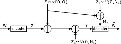
Figure 2: Channel model with an observation of $\mathbf{S}$ at the receiver.

Fig. 2 shows the channel model when the observation of $\mathbf{S}$ is only available at the receiver. This channel is equivalent to our original model when $N_{1}\rightarrow\infty$. The capacity of the channel is given by

$$I(X;Y,M_{2})=\frac{1}{2}\log\left(1+\frac{P}{Q\left(\frac{N_{2}}{Q+N_{2}}\right)+N_{0}}\right).$$ (31)

III-A2 Noisy estimate at transmitter only: Generalization of Dirty Paper Coding

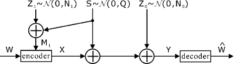
Figure 3: Channel model with an observation of $\mathbf{S}$ at transmitter.

Fig. 3 shows the channel model when the observation of $\mathbf{S}$ is only available at the transmitter. This is a special case of our original model with $N_{2}\rightarrow\infty$. The capacity of the channel is

$$I(X;Y|M_{1})=\frac{1}{2}\log\left(1+\frac{P}{Q\left(\frac{N_{1}}{Q+N_{1}}\right)+N_{0}}\right).$$ (32)

The achievability can be easily shown following the same steps as in Section II-C with $N_{2}\rightarrow\infty$. Note that when $N_{1}=0$, the channel model further reduces to Costa’s dirty paper coding channel model [1].

Remarks:

1) In [1], Costa showed the surprising fact that the channel capacity with additive Gaussian interference known to the transmitter only is the same as the channel capacity with the interference known to the receiver only. This paper extends that result to the case of noisy interference. Indeed, by setting $N_{1}=N_{2}$ in (31) and (32), we can see that the capacity with noisy interference known to transmitter only equals the capacity with a statistically similar noisy interference known to receiver only.

2) From (32), one may intuitively interpret the effect of knowledge of $M_{1}$ at the transmitter. Indeed, a fraction $\frac{Q}{Q+N_{1}}$ of the interfering power can be canceled using the proposed coding scheme. The remaining $\frac{N_{1}}{Q+N_{1}}$ fraction of the interfering power, $Q$, is treated as ‘residual’ noise. Thus, unlike Costa’s result [1], the capacity in this case depends on the power $Q$ of the interfering source: For a fixed $N_{1}$, as $Q$ increases, the capacity decreases. The capacity approaches $\frac{1}{2}\log\left(1+\frac{P}{N_{1}+N_{0}}\right)$ with $Q\rightarrow\infty$.

III-B Multiple Independent Observations

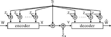
Figure 4: Channel model with multiple independent observations of $\mathbf{S}$.

Let there be $n_{1}$ independent observations $\mathbf{M}_{1},\mathbf{M}_{2},\ldots,$ $\mathbf{M}_{n_{1}}$ of $\mathbf{S}$ at the transmitter and $n_{2}$ independent observations $\mathbf{M}_{n_{1}+1},\mathbf{M}_{n_{1}+2},\ldots,\mathbf{M}_{n_{1}+n_{2}}$ at the receiver, as shown in Fig. 4. Similar to Section II-B, an upper bound on the capacity of this channel can be computed as

$$~{}I(X;Y|M_{1},M_{2},\ldots,M_{n_{1}+n_{2}})$$

$$\leq ~{}I(X;Y,M_{1},M_{2},\ldots,M_{n_{1}+n_{2}})$$

$$= ~{}H(X)+H(Y,M_{1},M_{2},\ldots,M_{n_{1}+n_{2}})\quad\quad\quad~{}\quad\quad\quad$$

$$-H(X,Y,M_{1},M_{2},\ldots,M_{n_{1}+n_{2}})$$

$$= ~{}\frac{1}{2}\log(2\pi e)^{n_{1}+n_{2}+2}\cdot$$

$$~{}P\left|\begin{array}[]{cccc}P+Q+N_{0}&Q&\cdots&Q\\ Q&Q+N_{1}&\ddots&\vdots\\ \vdots&\ddots&\ddots&Q\\ Q&\cdots&Q&Q+N_{n_{1}+n_{2}}\end{array}\right|$$ (37)

$$-\frac{1}{2}\log(2\pi e)^{n_{1}+n_{2}+2}\cdot$$

$$~{}\left|\begin{array}[]{ccccc}P&P&0&\cdots&0\\ P&P+Q+N_{0}&Q&\cdots&Q\\ 0&Q&Q+N_{1}&\ddots&\vdots\\ \vdots&\vdots&\ddots&\ddots&Q\\ 0&Q&\cdots&Q&Q+N_{n_{1}+n_{2}}\end{array}\right|$$ (43)

$$= ~{}\frac{1}{2}\log\left(1+\frac{P}{\hat{\mu}Q+N_{0}}\right)$$ (44)

where $\hat{\mu}=\frac{1}{1+\frac{Q}{N_{1}}+\frac{Q}{N_{2}}+\cdots+\frac{Q}{N_{n_{1}+n_{2}}}}$ and $N_{1},N_{2},\ldots,N_{n_{1}+n_{2}}$ are the variances of the Gaussian noise variables, $Z_{1},Z_{2},\ldots,Z_{n_{1}+n_{2}}$, corresponding to the $n_{1}+n_{2}$ observations.

Achievability of capacity: To show the achievability, the coding process follows the same random coding argument as in Section II-C. The main difference is that in this case, we first construct one estimate of the interference at the transmitter (similarly at the receiver) based on the multiple noisy observations and then use this estimate in the coding process. Thus, we omit the detailed development and show only the main steps.

At the transmitter, upon receipt of the $n_{1}$ independent observations, the encoder makes a maximum likelihood estimation (MLE) of $\mathbf{S}$, which is given as

$$\hat{S}_{1}=\arg{\underset{S}{\max}}f_{S}(M_{1},M_{2},\ldots,M_{n_{1}}|S)$$ (45)

where

$$f_{S}(M_{1},M_{2},\ldots,M_{n_{1}}|S)=\prod_{l=1}^{n_{1}}\frac{1}{\sqrt{2\pi N_{l}}}\exp\left(-\frac{(M_{l}-S)^{2}}{2N_{l}}\right).$$ (46)

Taking logarithm on both side of (46) and differentiating with respect to $S$, the estimate, $\hat{S}_{1}$, which maximizes $f_{S}$ is found to be

$$\hat{S}_{1}=\sum_{l=1}^{n_{1}}\frac{M_{l}}{\sum_{k=1}^{n_{1}}\frac{N_{l}}{N_{k}}}=S+\sum_{l=1}^{n_{1}}\frac{Z_{l}}{\sum_{k=1}^{n_{1}}\frac{N_{l}}{N_{k}}}.$$ (47)

Thus, the variance of the estimation error at the transmitter can be computed as

$$\hat{N}_{1}=\text{Var}\left(\sum_{l=1}^{n_{1}}\frac{Z_{l}}{\sum_{k=1}^{n_{1}}\frac{N_{l}}{N_{k}}}\right)=\frac{1}{\sum_{l=1}^{n_{1}}\frac{1}{N_{l}}}.$$ (48)

Similarly, at the receiver, the decoder also computes the MLE, $\hat{S}_{2}$ of $S$ based on the $n_{2}$ independent observations. The variance of the estimation error at the receiver is given by

$$\hat{N}_{2}=\frac{1}{\sum_{l=n_{1}+1}^{n_{1}+n_{2}}\frac{1}{N_{l}}}.$$ (49)

Thus, using MLE, the multiple observations is equivalent to one observation each at the transmitter and receiver with estimation noise variance $\hat{N}_{1}$ and $\hat{N}_{2}$. Essentially, the construction of the auxiliary variable ${U}$ is similar to that in Section II-C using $\hat{N}_{1}$ and $\hat{N}_{2}$, i.e., ${U}=X+\alpha\hat{S}_{1}$. The achievable rate, $R^{*}$, can then be found by substituting $\hat{N}_{1}$ and $\hat{N}_{2}$ instead of $N_{1}$ and $N_{2}$, respectively, in (30) and is given by,

$$R^{*}=\frac{1}{2}\log\left(1+\frac{P}{\hat{\mu}Q+N_{0}}\right)$$ (50)

where $\hat{\mu}=\frac{1}{1+\frac{Q}{\hat{N}_{1}}+\frac{Q}{\hat{N}_{2}}}=\frac{1}{1+\frac{Q}{N_{1}}+\frac{Q}{N_{2}}+\cdots+\frac{Q}{N_{n_{1}+n_{2}}}}$. Clearly, $R^{*}$ is the same as the upper bound on capacity given in (44).

Remark: It is easy to see that the capacity expression is symmetric in the noise variances at the transmitter and receiver. In other words, having all the $n_{1}+n_{2}$ observations at the transmitter would result in the same capacity. Thus, the observations of $\mathbf{S}$ made at the transmitter and the receiver are equivalent in achievable rate, as long as the corrupting Gaussian noises have the same statistics. Further, if there is an extra independent observation of $\mathbf{S}$ with corrupting noise variance $N_{n_{1}+n_{2}+1}$, the fraction $\hat{\mu}$ in (50) decreases to $\frac{1}{1+\frac{Q}{N_{1}}+\frac{Q}{N_{2}}+\cdots+\frac{Q}{N_{n_{1}+n_{2}}}+\frac{Q}{N_{n_{1}+n_{2}+1}}}$. Thus, the irremovable part of the noise power $Q$ decreases and the achievable rate increases. It is clear that it does not matter whether this extra observation is obtained at the transmitter or the receiver.

IV CONCLUSION

In this paper, we derived the capacity region for a Gaussian noise channel with additive Gaussian interference, when noisy estimates of the interference are known at the transmitter and receiver. Our results indicate that knowledge of the interference at the transmitter gives the same capacity as knowledge of statistically similar interference at the receiver. As noted earlier, all results in this paper are derived assuming non-causal knowledge of the noisy interference. Studying capacity with causal knowledge of the interference should be investigated in future work.

References

- [1] M. H. M. Costa, “Writing on dirty paper,” IEEE Trans. Inform. Theory, vol. 29, pp. 439–441, May 1983.
- [2] S. I. Gel’fand and M. Pinsker, “Coding for channel with random parameters,” Problems of Control and Inform. Theory, vol. 9, no. 1, pp. 19–31, 1980.
- [3] A. E. Gamal and C. Heegard, “On the capacity of computer memories with defects,” IEEE Trans. Inform. Theory, vol. 29, pp. 731–739, Sept. 1983.
- [4] T. M. Cover and M. Chiang, “Duality between channel capacity and rate distortion with two-sided state information,” IEEE Trans. Inform. Theory, pp. 1629–1638, June 2002.
- [5] W. Yu, A. Sutivong, D. Julian, T. M. Cover, and M. Chiang, “Writing on colored paper,” in Proc. of IEEE ISIT, p. 302, June 2001.
- [6] A. S. Cohen and A. Lapidoth, “Generalized writing on dirty paper,” in Proc. of IEEE ISIT, p. 227, June-July 2002.
- [7] U. Erez, S. Shamai, and R. Zamir, “Capacity and lattice strategies for cancelling known interference,” IEEE Trans. Inform. Theory, pp. 3820–3833, Nov. 2005.
- [8] V. Licks, F. Ourique, R. Jordan, and G. Hekleman, “Performance loss of dirty-paper codes in additive white Gaussian noise and jitter channels,” IEEE Workshop on Statistical Signal Processing, pp. 230–233, Sept.-Oct. 2003.
- [9] B. Chen and G. W. Wornell, “Quantization index modulation: a class of provably good methods for digital watermarking and information embedding,” IEEE Trans. Inform. Theory, pp. 1423–1443, May 2001.
- [10] A. S. Cohen and A. Lapidoth, “The Gaussian watermarking game,” IEEE Trans. Inform. Theory, pp. 1639–1667, June 2002.
- [11] G. Caire and S. Shamai, “On achievable rates in a multi-antenna Gaussian broadcast channel,” in Proc. of IEEE ISIT, p. 147, June 2001.
- [12] W. Yu and J. M. Cioffi, “Trellis precoding for the broadcast channel,” in Proc. of IEEE GlobeCom, pp. 1344–1348, Nov. 2001.
- [13] M. Mazzotti and Z. Xiong, “Effects of noisy side information at the decoder in dirty-paper and dirty-tape coding,” in Proc. of Inform. Theory Workshop, pp. 390–394, Oct. 2006.
- [14] T. M. Cover and J. A. Thomas, Elements of Information Theory. Wiley-Interscience, 2nd ed., 2006.