A Fresh Look into the Neutron EDM and Magnetic Susceptibility

Abstract

We reexamine the estimate of the neutron Electric Dipole Moment (NEDM) from chiral and QCD spectral sum rules (QSSR) approaches. In the former, we evaluate the pion mass corrections which are about 5% of the leading Log. results. However, the chiral estimate can be affected by the unknown value of the renormalizaton scale $\nu$. For QSSR, we analyze the effect of the nucleon interpolating currents on the existing predictions. We conclude that previous QSSR results are not obtained within the optimal choice of these operators, which lead to an overestimate of these results by about a factor 4. The weakest upper bound $|\theta|\leq 2\times 10^{-9}$ for the strong $CP$-violating angle is obtained from QSSR, while the strongest upper bound $|\theta|\leq 1.3\times 10^{-10}$ comes from the chiral approach evaluated at the scale $\nu=M_{N}$. We also re-estimate the proton magnetic susceptibility, which is an important input in the QSSR estimate of the NEDM.

1 Introduction

The Lagrangian of Yang-Mills theory contains, in addition to the usual term, also a topological term:

$${\cal L}=-\frac{1}{4}F^{a}_{\mu\nu}F^{a\mu\nu}-\theta q(x)~{},$$ (1)

where $q(x)$ is the topological charge density given by:

$$q(x)=\frac{g^{2}}{32\pi^{2}}F_{\mu\nu}^{a}{\tilde{F}}^{a\mu\nu}~{}~{}~{}:~{}~{}~{}{\tilde{F}}^{\mu\nu}=\frac{1}{2}\epsilon^{\mu\nu\rho\sigma}F_{\rho\sigma}~{}.$$ (2)

The additional term violates the invariance under $CP$. This is called strong $CP$ violation [1] to distinguish it from the $CP$ violation present in the weak and electromagnetic sector of the Standard Model. Experiments, however, do not show any violation of strong $CP$ and require a very small value for $|\theta|<2\times 10^{-9}$ as we shall see later on. In this paper we shall determine the dependence of physical quantities on $\theta$ and study the processes that violate strong $CP$. For this purpose, we reevaluate the neutron electric dipole moment (NEDM) which depends on the $\pi NN$ coupling which violates CP.

2 Improved chiral estimate of the NEMD

An elegant way of doing this is to use the low energy effective Lagrangian of QCD that contains the fields of the pseudoscalar mesons and baryons instead of the original quarks and gluons. This is due to the fact that in the effective Lagrangian the effect of the axial $U(1)$ anomaly is explicitly displayed and because of this the amplitudes for the hadronic processes can be easily computed. This Lagrangian cannot be explicitly derived from the fundamental QCD Lagrangian as in the $CP^{N-1}$ model (see e.g. Ref. [2, 3] and References therein), but can only be constructed requiring that it has the same anomalous and non-anomalous symmetries of the fundamental QCD Lagrangian. The expressions of the QCD effective Lagrangian describing pseudoscalar mesons and including the $U(1)$ anomaly are given in [4, 5, 6, 7, 8, 9, 10, 11] and the review in Ref. [2, 3].

$\bullet~{}$Estimate of the $\pi NN$ couplings

The $\pi NN$ couplings are defined as :

$${\cal L}_{\pi NN}=\sqrt{2}\pi\bar{N}{\bf\tau}\left(i\gamma_{5}g_{\pi NN}+\bar{g}_{\pi NN}\right)N~{},$$ (3)

where ${\bf\tau}$ are isospin Pauli matrices.

The $CP$-conserving coupling is well measured :

$$g_{\pi NN}=13.4.$$ (4)

The $CP$-violating coupling $\bar{g}_{\pi NN}$ can be obtained using an effective Lagrangian approach, though this approach for estimating the coupling can be questionable. It reads [7, 3]:

$${\bar{g}}_{\pi NN}=-\frac{m_{u}m_{d}\theta}{f_{\pi}(m_{u}+m_{d})(m_{s}-m)}\left(m_{\Xi}-m_{\Sigma}\right)\times$$

$$\left[1+\frac{3m(m_{\Sigma}-m_{\Lambda})}{2(m_{s}-m)m_{N}}\right]$$ (5)

with: $2m\equiv(m_{u}+m_{d})$. We shall use the ChPT mass ratio [15]:

$$r_{3}\equiv\frac{2m_{s}}{(m_{u}+m_{d})}=24.4\pm 1.5~{},$$ (6)

which is confirmed by the QSSR estimates of the quark mass absolute values in units of MeV [12, 13]:

$$m_{u}(2)=(2.8\pm 0.2)~{},~{}~{}~{}m_{d}(2)=(5.1\pm 0.4)~{},$$ (7)

and:

$$~{}~{}~{}m_{s}(2)=(96.3\pm 17.5)~{}.$$ (8)

Using $f_{\pi}=92.46$ MeV, one can deduce:

$$\bar{g}_{\pi NN}=(0.0282\pm 0.0071)\theta~{},$$ (9)

which is relatively small compared to $g_{\pi NN}$. One can also note that the chiral correction is about 0.5% of the leading order expression given in Ref. [7]. We have added an error of about 25% as a guess of the systematics of the method based on its deviation for predicting the value of the measured $CP$-conserving coupling .

$\bullet~{}$The NEDM from chiral and ChPT approaches

To first order in $\theta$, the neutron electric dipole moment (NDEM) $D_{N}$ is given by:

$$V_{\mu} \equiv {\cal T}\langle n(p_{f})|J_{\mu}(0)~{}i\int d^{4}x\delta{\cal L}_{CP}(x)|n(p_{i})\rangle$$ (10)

$$= -\left(iD_{N}\right)\bar{u}(p_{f})\sigma_{\mu\nu}k^{\nu}\gamma_{5}u(p_{i})+{\cal O}(k^{2})~{},$$

where : $k\equiv p_{f}-p_{i}$ is the photon momentum and:

$$\delta{\cal L}_{CP}(x)=\bar{q}(i\gamma_{5}){\cal A}q~{},$$ (11)

with A a 3-dimension hermitian matrix acting on the flavour space (u, d, s) and $\sigma_{\mu\nu}\equiv({1/2})\left(\gamma_{\mu}\gamma_{\nu}-\gamma_{\nu}\gamma_{\mu}\right)~{}.$ In order to extract $D_{N}$, we use the Gordon decomposition for the axial current:

$$\bar{u}(p+k)\gamma_{5}\sigma_{\mu\nu}k^{\nu}u(p)=...+\bar{u}(p+k)\gamma_{5}(2p+k)_{\mu}u(p).$$ (12)

The lowest order contribution to $D_{N}$ comes from the diagrams in Figs 1 and 2. Using the expression of the $\pi\pi\gamma$ vertex :

$$\langle\pi^{-}(p+k)|J_{\mu}|\pi^{-}(p)\rangle=-(2p+k)_{\mu}+{\cal O}(k^{2})~{},$$ (13)

the evaluation of the previous diagrams can be expressed as:

$$D_{N}= (-1)^{3}\bar{g}_{\pi NN}g_{\pi NN}\left({2M_{N}\over M_{N}^{2}}\right)\left({1\over 16\pi^{2}}\right)\times$$ (14)

$$2\left\{I^{(1)}+I^{(2)}\right\}$$

where $I^{(n)}$ are integrals over Feynman parameters coming from Figs 1 and 2. Fig 1 gives:

$$I^{(1)} \equiv \int_{0}^{1}xdx\int_{0}^{1}dy~{}{x(1-y)\over x^{2}(1-y)^{2}+a\Big{[}1-x(1-y)\Big{]}}$$ (15)

$$= -1-{\log{a}\over 2}\left(1-a\right)+f(a)$$

with:

$$f(a) = {a\left(3-a\right)\over\sqrt{a(4-a)}}\Big{\{}\arctan{\Big{[}{2-a\over\sqrt{a(4-a)}}\Big{]}}+$$ (16)

$$\arctan{\Big{[}{a\over\sqrt{a(4-a)}}\Big{]}}\Big{\}}$$

$$\simeq {3\over 4}\left(\pi\sqrt{a}-a\right)-{5\over 32}\pi a^{3/2}+\ldots~{},$$

and where:

$$a\equiv\left(m_{\pi}/M_{N}\right)^{2}~{}.$$ (17)

One can notice that the term $\log{a}$ appears naturally in the unexpanded full expression without an arbitrary choice of the cut-off $M_{N}$. One can also note the non-analytic terms $\sqrt{a}$ and $a^{3/2}$. In the same way, Fig 2 gives:

$$I^{(2)} \equiv \int_{0}^{1}xdx\int_{0}^{1}dy{x\over x^{2}+a(1-x)}$$ (18)

$$= 1+{(-2+a)a\over\sqrt{(4-a)a}}\Big{\{}\arctan{(2-a)\over\sqrt{(4-a)a}}-$$

$$\arctan{a\over\sqrt{(4-a)a}}\Big{\}}-{a\over 2}\log{a}$$

$$= 1-{\pi\over 2}\sqrt{a}+{a\over 2}\left(3-\log{a}\right)+{3\over 16}\pi a^{3/2}.$$

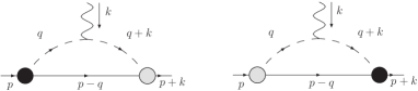
Figure 1: 1st class of diagrams contributing to $D_{N}$.

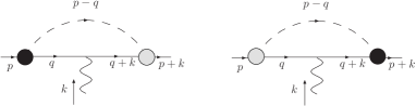
Figure 2: 2nd class of diagrams contributing to $D_{N}$.

$\bullet~{}$Results and discussions

Adding the previous Feynman integrals $I^{(1)}$ and $I^{(2)}$ [ Eqs. (15) and (18)] into the expression of NEDM in Eq. (14), the NEDM from chiral approach reads:

$$D_{N}|_{\rm chiral} = {\bar{g}_{\pi NN}g_{\pi NN}\over M_{N}}\left({1\over 4\pi^{2}}\right)\times\Bigg{\{}-{\log{a}\over 2}+$$ (19)

$$0+{1\over 4}\left(\pi\sqrt{a}+3a\right)+\ldots\Bigg{\}}~{}.$$

The leading-log term agrees with the original result in Ref  [7]. The cancellation of the constant terms have been also noticed in [16]. In addtion, we also have a cancellation of the $a\log{a}$ term, which implies small mass corrections (about 5%). Our result demonstrates the accuracy of the leading-log approximation used in Ref. [7]. It also shows that the scale, appearing in the leading-$\log{a}$ term, is the mass of the nucleon but not any arbitrary cut-off scale, because this term appears before the expansion in $a$ [see Eq. (15)]. This leads to the prediction:

$$D_{N}|_{\rm chiral} = (20\pm 5)\times 10^{-3}\theta~{}{\rm GeV}^{-1}~{},$$ (20)

$$= (40\pm 10)\times 10^{-17}\theta~{}{\rm cm}~{}.$$

However, within Chiral Perturbation Theory (ChPT), the addition of counterterms in the effective Lagrangian induces a $\log(M_{N}/\nu)^{2}$-term and leads to the (renormalized) NEDM expression [16]:

$$D_{N}(\nu)|_{\rm ChPT}={\bar{g}_{\pi NN}g_{\pi NN}\over M_{N}}\left({1\over 4\pi^{2}}\right)\Bigg{\{}\log{\nu\over m_{\pi}}+k\Bigg{\}}$$ (21)

where $\nu$ is an arbitrary hadronic scale and $k$ an unknown constant. This result indicates that, only the coefficient of the $\log m_{\pi}$ term is model independent.

For a conservative estimate and for a model independent result, we keep only the $\log m_{\pi}$ term and move, like in [16], the scale $\nu$ above $m_{\pi}$ from the value of the constituent quark mass, which we take to be about $(M_{N}/3)$ (within a 30% error), to $M_{N}=940$ MeV. Using the values of the parameters in Eqs. (4) and (9), one obtains, in units of the electric charge $e$:

$$D_{N}(\nu) = (2.7\sim 23.8)\times 10^{-3}\theta~{}{\rm GeV}^{-1}~{},$$ (22)

$$= (5.4\sim 47.6)\times 10^{-17}\theta~{}{\rm cm}~{},$$

where the range takes into account the assumed 25% systematic uncertainties for estimating $\bar{g}_{\pi NN}$ and the assumed 30% one for the value of the quark constituent mass. The value in Eq. (20) corresponds to the value $\nu=M_{N}$ and where the small chiral mass corrections have been included. One can notice that the width of the range depends strongly on the unknown value of $\nu$, and where a fine tuning is obtained for its low values.

3 NEDM and Magnetic Susceptibility from QSSR

Alternative estimates of the NEDM have been done using QCD spectral sum rules [17]. We shall re-examine these results in this section and present some alternative new sum rules.
The analysis is based on the baryon two-point correlator put in a background with nonzero $\theta$ and electromagnetic field $F_{\mu\nu}$:

$$S(q^{2})|_{\theta,~{}F}=i\int d^{4}x~{}e^{iqx}\langle 0|{\cal T}N(x)\bar{N}(0)|0\rangle|_{\theta,~{}F}$$ (23)

$N$ is the nucleon operators which can be written in general as  :

$$N(x)\equiv 2\left\{\left(\psi C\gamma^{5}\psi\right)\psi+b\left(\psi C\psi\right)\gamma^{5}\right\}~{},$$ (24)

where $C$ is the charge conjugate; $\psi$ is the quark field; $b$ is (a priori) an arbitrary mixing between the two operators: $b=0$ in the non-relativistic limit, which is the choice used in different lattice calculations [18]. Originally, Ioffe [19] has used the choice $b=-1$ in the 1st QSSR applications to the nucleon channel, which he has justified for a better convergence of the QCD series in the OPE. In [20, 21] , a more general analysis has been performed by letting $b$ as a free parameter and then looks for the $b$-value where the result is less sensitive to the variation of $b$. From the overall fit using different form of the sum rules, the optimal result for the nucleon mass and residue have been obtained for $b=-1/5$, which can be qualitatively understood by taking the zero of the derivative in $b$ when retaining only the lowest order contribution.
For the analysis of the NEDM, Ref. [17] has used a value $b=1$, which differs completely from the previous choices. Within this choice, the authors impose the zero coefficient of an non-analytic mass- Log. in the next $1/Q^{2}$-corrections $(q^{2}\equiv-Q^{2})$ to the lowest order contribution. However, the vanishing of the mass- Log. to leading order does not (a priori) guarantee the absence of this contribution to higher orders. In the following, we shall test the stability of the existing results versus the variation of $b$.

$\bullet~{}$Expression of the two-point correlator

For the forthcoming analysis, we shall keep the coefficient of the term $\{\tilde{F}_{\mu\nu}\sigma^{\mu\nu},\gamma_{\mu}q^{\mu}\}~{},$ in the Lorentz decomposition of the nucleon two-point correlator given in Eq. (3) (some alternative choices are also possible). The QCD expression reads [17] :

$$S(Q^{2})|_{\theta,~{}F}^{\rm th}=-\theta m^{*}\langle\psi\psi\rangle\left({1\over 32\pi^{2}}\right)\Bigg{\{}-\chi C_{0}\ln{Q^{2}\over\nu^{2}}+$$

$$\Big{[}C_{2a}\left(\ln{Q^{2}\over\nu_{\chi}^{2}}-1\right)+C_{2b}\Big{]}{1\over Q^{2}}+{\cal O}\left({1\over Q^{4}}\right)\Bigg{\}}$$ (25)

$\nu$ and $\nu_{\chi}$ correspond to an UV and a small mass arbitrary subtractions; $\langle\bar{\psi}\psi\rangle$ is the quark condensate. The coefficient-functions are:

$$C_{0}=(b+1)^{2}(4e_{d}-e_{u})~{},$$

$$C_{2a}=-4(b-1)^{2}e_{d}\left(1+{1\over 4}(2\kappa+\xi)\right)~{},$$

$$C_{2b}=-{\xi\over 2}\Big{[}(4b^{2}-4b+2)e_{d}+(3b^{2}+2b+1)e_{u}\Big{]}~{},$$ (26)

where $e_{u},~{}e_{d}$ are the electric charge of the $u$ and $d$ quarks in units of e. $\chi,~{}\zeta,~{}\xi$ are the magnetic susceptibilities of the QCD condensates which encode the electromagnetic field dependence of the two-point correlator. In units of $e$, they are defined as [22]:

$$\langle 0|\bar{\psi}\sigma_{\mu\nu}\psi|0\rangle|_{F} = e_{q}\chi F_{\mu\nu}\langle\bar{\psi}\psi\rangle~{},$$

$$g\langle 0|\bar{\psi}{\lambda_{a}\over 2}G^{a}_{\mu\nu}\psi|0\rangle|_{F} = e_{q}\kappa F_{\mu\nu}\langle\bar{\psi}\psi\rangle~{},$$

$$g\langle 0|\bar{\psi}\gamma_{5}{\lambda_{a}\over 2}G^{a}_{\mu\nu}\psi|0\rangle|_{F} = ie_{q}\xi F_{\mu\nu}\langle\bar{\psi}\psi\rangle~{},$$ (27)

where $g$ is the QCD coupling and $G^{a}_{\mu\nu}$ the gluon field strength. The size of these magnetic susceptibilities have been estimated in the literature using different methods. The values [23] :

$$\kappa\simeq-(0.34\pm 0.10)~{},~{}~{}~{}~{}~{}~{}~{}~{}\xi\simeq-(0.74\pm 0.2)~{},$$ (28)

induce (a posteriori) small numerical corrections in the present analysis and will not be reconsidered. On the contrary, the dominant contribution comes from $\chi$, which is not known with a good accuracy:

$$\chi[{\rm GeV}^{-2}]= -8=-{N_{c}\over 4\pi^{2}f_{\pi}^{2}}:~{}{\rm Triangle~{}anomaly}\cite[cite]{[\@@bibref{}{VAIN}{}{}]}$$ (29)

$$-8,~{}-6~{}~{}{\rm Laplace~{}SR(LSR)}\cite[cite]{[\@@bibref{}{IOFFE2,WYLER}{}{}]}$$

$$-3.3~{}~{}{\rm Light~{}cone~{}SR}\cite[cite]{[\@@bibref{}{BALL}{}{}]}~{},$$

which we shall reconsider later on. Our analysis gives the value in Eq. (43), which is in better agreement with the one obtained in [22, 24].

The phenomenological part of the correlator can be parametrized in the zero width approximation by:

$$S(q^{2})|_{\theta,~{}F}^{exp} = {\lambda_{N}^{2}M_{N}D_{N}\over(q^{2}-M^{2}_{N})^{2}}+{A\over q^{2}-M_{N}^{2}}+$$ (30)

$$``{\rm QCD~{}continuum}"~{},$$

where $\lambda_{N}$ is the nucleon coupling to its corresponding current; A is an arbitrary coupling which parametrizes the single pole contributions; “QCD continuum” stands from the QCD smearing of excited state contributions and comes from the discontinuity of the QCD expression.

$\bullet~{}$Estimate of the Magnetic susceptibility

Considering the nucleon two-point correlator in Eq. (3) in presence of an external electromagnetic field, one can derive the following LSR (neglecting anomalous dimensions) for each invariants related to the structure $(\sigma_{\mu\nu}\hat{p}+\hat{p}\sigma_{\mu\nu})$ and $i(p_{\mu}\gamma_{\nu}-p_{\nu}\gamma_{\mu})$ [22] (hereafter referred as IS):

$${\cal L}^{\sigma}_{p} \equiv e_{u}M^{4}(1-\rho_{1})+{a^{2}\over 3M^{2}}\Bigg{\{}-(e_{d}+{2\over 3}e_{u})+$$ (31)

$${1\over 3}e_{u}(\kappa-2\zeta)-2e_{u}\chi(M^{2}-{1\over 8}M_{0}^{2})\Bigg{\}}$$

$$= {1\over 4}\tilde{\lambda}_{N}^{2}e^{-M_{N}^{2}/M^{2}}\left({\mu_{p}\over M^{2}}+A_{p}\right)~{},$$

$${\cal L}^{\gamma}_{p} \equiv aM_{N}\Bigg{\{}e_{u}+{1\over 2}e_{d}+$$ (32)

$${1\over 3}e_{d}\chi M^{2}\Big{[}(1-\rho_{0})+{b\over 24M^{4}}\Big{]}\Bigg{\}}$$

$$= {1\over 4}\tilde{\lambda}_{N}^{2}e^{-M_{N}^{2}/M^{2}}\left({\mu^{a}_{p}\over M^{2}}+B_{p}\right)~{},$$

where $M^{2}\equiv 1/\tau$ is the SR variable; $M_{N}=0.946$ GeV is the proton mass; $a\equiv 4\pi^{2}|\langle 0|\bar{\psi}\psi|0\rangle|$; $b=4\pi\langle 0|\alpha_{s}G^{2}|0\rangle\simeq 0.87$ GeV⁴ [29, 13] are the quark and gluon condensates; $M^{2}_{0}=0.8$ GeV² [19, 20, 21, 30, 13] parametrizes the mixed quark-gluon condensate: $\langle 0|\bar{\psi}\sigma_{\mu\nu}(\lambda^{a}/2)G_{a}^{\mu\nu}\psi|0\rangle=M^{2}_{0}\langle 0|\bar{\psi}\psi|0\rangle$; The QCD continuum contribution from a threshold $t_{c}$ is quantified as:

$$\rho_{n}=e^{-t_{c}\tau}\left(1+t_{c}\tau+{(t_{c}\tau)^{2}\over 2}+...+{(t_{c}\tau)^{n}\over n!}\right)~{};$$ (33)

$A_{p},~{}B_{p}$ are the single proton pole coupling to the two-point correlator, while $\tilde{\lambda}_{N}^{2}\equiv 32\pi^{4}\lambda^{2}_{N}$ is the coupling of the double proton pole; $\kappa$, $\zeta$ and $\chi$ have been defined in Eq. (27); $\mu_{p}$ and $\mu_{p}^{a}$ are the proton magnetic and anomalous magnetic moments. The sum rules for the neutron can be deduced from Eqs. (31) and (32) by the substitution:

$$e_{d}\leftrightarrow e_{u}~{};~{}~{}~{}~{}~{}~{}~{}\mu_{p},~{}\mu_{p}^{a}\rightarrow~{}\mu_{n}~{};~{}~{}~{}~{}~{}~{}~{}A_{p},~{}B_{p}\rightarrow A_{n},~{}B_{n}~{}.$$ (34)

Multiplying Eqs. (31) and (32) by $e_{d}$ and each corresponding neutron sum rule by $e_{u}$ and then subtracting the proton and the corresponding neutron sum rules, IS deduce:

$$\mu_{p}e_{d}-\mu_{n}e_{u}+(A_{p}e_{d}-A_{n}e_{u})\tau^{-1}=$$

$${4a^{2}\over 3\tilde{\lambda}_{N}^{2}}e^{M^{2}_{N}\tau}(e_{u}^{2}-e_{d}^{2})~{},$$

$$\mu^{a}_{p}e_{u}-\mu_{n}e_{d}+(B_{p}e_{u}-B_{n}e_{d})\tau^{-1}=$$

$${4aM_{N}\tau^{-1}\over\tilde{\lambda}_{N}^{2}}e^{M^{2}_{N}\tau}(e_{u}^{2}-e_{d}^{2})~{}.$$ (35)

In order to eliminate the single pole contribution, IS apply, to both sides of Eq. (35), the operator:

$${\cal L}_{01}\equiv\left(1+\tau{\partial\over\partial{\tau}}\right)~{}.$$ (36)

Using the LSR expression of the proton coupling $\lambda_{N}$ from the $M_{N}$-component $F_{2}$ of the two-point correlator [19, 20, 21]:

$$\tilde{\lambda}^{2}_{N}\simeq{2a\tau^{-2}\over M_{N}}e^{M^{2}_{N}\tau}~{},$$ (37)

IS deduces for $\tau^{-1}\approx M^{2}_{N}$:

$$\mu_{p} \approx {8\over 3}\left(1+{1\over 6}{a\over M^{3}_{N}}\right)\approx 2.96~{},$$

$$\mu_{n} \approx -{4\over 3}\left(1+{2\over 3}{a\over M^{3}_{N}}\right)\approx-1.93~{},$$ (38)

in remarkable agreement with the experimental values:

$$\mu_{p}^{exp}=2.79~{},~{}~{}~{}~{}~{}~{}~{}~{}~{}\mu_{n}^{exp}=-1.91~{},$$ (39)

despite the crude LO approximation used for getting these predictions. Including the OPE and anomalous dimension corrections, IS deduce, from Eq. (35), the predictions :

$$\mu_{p}^{exp}=3.0~{},~{}~{}~{}~{}~{}~{}~{}~{}~{}\mu_{n}^{exp}=-2.0~{}.$$ (40)

and the correlated value:

$$\chi\simeq-8~{}{\rm GeV}^{-2}~{},$$ (41)

for $\xi\approx\kappa\approx 0$ . However, by examining the LSR used by the authors, we notice that these sum rules do not satisfy $\tau$-stability criteria such that (a priori) there is no good argument for extracting an optimal result.
In order to check the previous result, we solve the two equations:

$$\chi={d\over d\tau}{\cal L}^{\sigma}_{p}~{}~{}~{}~{}~{}~{}{\rm and}~{}~{}~{}~{}~{}~{}~{}\chi={d\over d\tau}{\cal L}^{\gamma}_{p}~{},$$ (42)

for each given value of $t_{c}$. The functions ${\cal L}^{\sigma,\gamma}_{p}$ have been defined in Eqs. (31) and (32). We use the values of $\kappa$ and $\xi$ given in Eq. (28) but they do not affect much the conclusions like in the case of IS. The analysis is shown in Fig. 3, where a common solution is reached at $\tau=0.4$ GeV^-2, though the curves do not exhibit $\tau$-stability region.

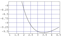
Figure 3: Analysis of $\chi$ using LSR for b=-1: a) $\tau$-dependence for $t_{c}=3.$ GeV²; b) $t_{c}$-dependence of the common solution in (a) for $\tau=.4$ GeV^-2.

Again like in the proton mass sum rule, the $t_{c}$-stability is reached around $t_{c}=3$ GeV² [21]. Taking as a conservative estimate the range of values $t_{c}=1.6\sim 3.$ GeV², where the lowest value corresponds to the beginning of $\tau$-stability for the determination of the proton mass, we deduce the optimal estimate:

$$\chi\simeq-(8.5\pm 1.0)~{}{\rm GeV}^{-2}~{},$$ (43)

in good agreement with the IS previous value [22] and the one in [24] using the quark triangle anomaly. At $\tau=0.4$ GeV^-2 where a common solution has been obtained, one expects a good convergence of the OPE and smaller effects of radiative corrections. We have used the choice $b=-1$ which we expect to give a reliable result like in the previous cases of the proton mass and $D_{N}$ discussed in the next section where the results are almost unchanged (within the errors) from $b=-1$ to the optimal value -1/5 obtained in the case of the proton mass [20, 21].

$\bullet~{}$Test of the LSR results of Ref. [17] for NEDM

From the previous QCD and phenomenological expressions of the two-point correlators, one can deduce the Borel/Laplace sum rule (LSR):

$${\cal L}(\tau) \equiv r(\tau)\equiv{1\over 2\theta m^{*}}\left(D_{N}+{A\tau^{-1}\over\lambda_{N}^{2}M_{N}}\right)$$ (44)

$$= -{\tau^{-2}\over 32\pi^{2}}\langle\bar{\psi}\psi\rangle e^{M^{2}_{N}\tau}\Bigg{\{}\chi C_{0}(1-\rho_{0})+\Bigg{[}C_{2a}\times$$

$$\Big{[}-\ln{(\tau\nu_{\chi}^{2})}+\gamma_{E}-1\Big{]}+C_{2b}\Bigg{]}\tau\Bigg{\}}~{},$$

where $\tau^{-1}\equiv M^{2}$ is the LSR variable. Ref. [17] uses either the value [19, 20, 21]:

$$\lambda_{N}^{2}\simeq{1\over(2\pi)^{4}}\left(1.05\pm 0.1\right){\rm GeV}^{6}~{},$$ (45)

or its LSR expression [19, 20, 21] from the $\hat{q}\equiv\gamma_{\mu}q^{\mu}$ part of the correlator:

$$(2\pi)^{4}\lambda^{2}_{N}e^{-\tau M_{N}^{2}}={5+2b+5b^{2}\over 64}\tau^{-3}\times$$

$$\Big{[}(1-\rho_{2})+\pi\langle\alpha_{s}G^{2}\rangle(1-\rho_{0})\tau^{2}\Big{]}~{}.$$ (46)

However, due to its high-dependence on $\tau$, this sum rule is much affected by the form of the continuum such that we shall not consider it. Instead, we shall consider either the value in Eq. (45), or the expression of the residue from the $M_{N}$ part of the correlator:

$$(2\pi)^{4}\lambda^{2}_{N}M_{N}e^{-\tau M_{N}^{2}}=-{\pi^{2}\over 4}\langle\bar{\psi}\psi\rangle\tau^{-2}\Big{[}(7-2b-5b^{2})$$

$$(1-\rho_{1})-3M^{2}_{0}\tau(1-b^{2})(1-\rho_{0})\Big{]}~{},$$ (47)

which has a lesser dependence in $\tau$.

We show the results in Fig 4 for the previous value of $\lambda_{N}^{2}$ and using, as in Ref. [17], $\langle\psi\psi\rangle=-[0.225~{}{\rm GeV}]^{3}$ for a better comparison.

– For the choice $b=1$ used in [17], one can see from Fig 4a that the optimal value is obtained at $M^{2}\equiv\tau^{-1}\simeq 0.5$ GeV², which is relatively low for justifying the convergence of both the OPE and the PT series in $\alpha_{s}$. Fig 4b shows, like in the case of the analysis of the proton mass, that the $t_{c}$ stability is reached at high-value of 3 GeV² but the estimate does not move much from the optimal value $t_{c}=1.6$ GeV² obtained in the proton mass sum rule [19, 20, 21]. In this case, one can deduce:

$$r|_{b=1}=-\chi(0.34\sim 0.36)~{}{\rm GeV}^{4}~{},$$ (48)

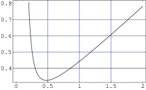
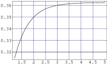
Figure 4: Analysis of $-r/\chi$ using LSR for b=1: a) $M^{2}$-dependence for $t_{c}=1.6$ GeV²; b) $t_{c}$-dependence for $M^{2}=.5$ GeV².

which reproduces the result of [17]. Assuming, like in Ref. [17], that the single pole contribution can be neglected (which we shall test in the next section), and using the value of $\chi=-5.7$ GeV^-2 used in [17], one can deduce from Eqs. (44) and (48) :

$$D_{N}|_{b=1}\approx 9\times 10^{-3}\theta~{}{\rm GeV}^{-1}~{}.$$ (49)

Though (almost) trivial, the previous test is necessary for calibrating our sum rule and for checking our inputs in the next analysis.

$\bullet~{}$New estimate of $A$ and choice of the nucleon currents

We shall reconsider the previous analysis by abandoning the choice $b=1$ for the nucleon current and by giving a new estimate of :

$$r_{A}(\tau)\equiv{1\over 2\theta m^{*}}\left({A\tau^{-1}\over\lambda_{N}^{2}M_{N}}\right)~{}.$$ (50)

This analysis is summarized in Fig. 5 where we have used the value of $\lambda_{N}$ in Eq. (45) and the running condensate value [12, 13, 26]:

$$\langle 0|\psi\psi|0\rangle(M)\simeq-[0.266~{}{\rm GeV}]^{3}\ln^{4/9}{\left(M/\Lambda\right)}~{},$$ (51)

with $\Lambda\simeq 350$ MeV for 3-flavours.

– One can notice that the result is optimal in $b$ for:

$$b\simeq-0.5~{},$$ (52)

and more conservatively in the range:

$$-1\leq b\leq 0~{},$$ (53)

which does not favour the choice $b=1$ used in [17]. The previous range includes the conventional choices: -1 in [19], -1/5 in [20, 21] and the non-relativistic limit $b=0$ used in lattice calculations [18].

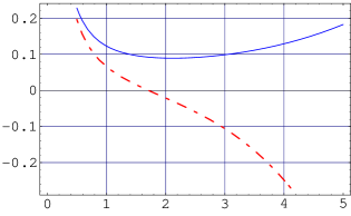
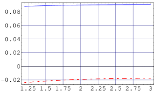
Figure 5: LSR analysis of $-r/\chi$ (red : dash-dotted curve) and $-r_{A}/\chi$ (blue : continuous curve) : a) $\tau\equiv 1/M^{2}$-dependence for $b=-0.5,~{}t_{c}=1.6$ GeV²; b) $t_{c}$ dependence for $b=-0.5,~{}\tau=2$ GeV^-2; c) $b$-dependence for $t_{c}=1.6$ GeV²,  $\tau=2$ GeV^-2

– The 2nd (important) assumption used in Ref. [17] is the neglect of the contribution of the single pole controlled by the parameter $A$. By inspecting the LSR in Eq. (44), one can isolate $A$ by working with the new LSR:

$${\cal L}_{1}(\tau)\equiv{d\over d\tau}{\cal L}~{}.$$ (54)

One can see in Fig. 5c that for all ranges of $b$, $r_{A}$ is much smaller than $r$ justifying the assumption of [17]. At the optimal range of $b$ values given previously, one can deduce :

$${r/\chi}=-0.09~{},~{}~{}~{}~{}~{}~{}~{}~{}~{}~{}~{}{r_{A}/\chi}=+0.02~{}.$$ (55)

Using the quark mass values in [12, 13] and the previous value of $\chi$ in Eq. (43), one gets:

$$D_{N}\simeq-0.11\chi\theta m^{*}\simeq(2.24\pm 0.12)\times 10^{-3}\theta~{}{\rm GeV}^{-1}~{}.$$ (56)

$\bullet~{}$Direct extraction of $D_{N}$ from a new LSR

– By inspecting the LSR in Eq. (44), one can also isolate $D_{N}$ by working with the LSR:

$${\cal L}_{2}(\tau)\equiv{d\over d\tau}\tau{\cal L}~{}.$$ (57)

We show the results of the analysis in Fig. 6.

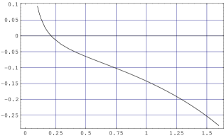
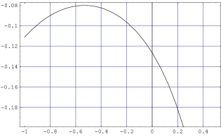
Figure 6: Analysis of $D_{N}$ using LSR a) $\tau\equiv 1/M^{2}$ in GeV^-2-dependence for $b=-0.5,~{}t_{c}=1.6$ GeV²; b) $b$-dependence for $\tau=0.75$ GeV^-2, $~{}t_{c}=1.6$ GeV²; c) $\nu_{\chi}$ -dependence of the optimal value in units of MeV.

One can notice that the sum rule stabilizes at $\tau\approx 0.75$ GeV^-2, which is smaller than in the previous analysis, showing a better convergence of the OPE.

– We also study the dependence of the result on the value of the IR scale $\nu_{\chi}$. The optimal value corresponds to:

$$\nu_{\chi}\simeq(80\sim 200)~{}{\rm MeV}~{},$$ (58)

which has the size of a typical IR chiral scale (pion or constituent quark mass).

Therefore, we deduce the optimal value:

$$D_{N} \simeq -(0.10\pm 0.03\pm 0.03)\chi\theta m^{*}$$ (59)

$$\simeq (2.06\pm 0.08)\times 10^{-3}\theta~{}{\rm GeV}^{-1}~{},$$

where the first (resp. second) error comes from the localization of the extremum in $\tau$ (resp.) of the $t_{c}$ values which we take to be $t_{c}=(1.6\pm 0.2)$ GeV² around the value obtained from the proton mass sum rule [20, 21].

$\bullet~{}$NEDM results and systematics from QSSR

The two results from the LSR are in good agreement and lead to the final estimate:

$$D_{N}|_{\rm QSSR}\simeq(2.15\pm 0.10)\times 10^{-3}\theta~{}{\rm GeV}^{-1}~{},$$ (60)

which agrees with the range spanned by the chiral and ChPT estimate in Eq. (20).

In order to analyze the systematic errors in the approach, we estimate using vertex sum rules the well measured coupling $g_{\pi NN}=13.4$. We use the symmetric configuration of the hadronic vertex in [27] from which, one obtains the LSR:

$$g_{\pi NN}(\lambda_{N}^{2}M_{N})(f_{\pi}m_{\pi}^{2})\tau^{3}e^{-M^{2}_{N}\tau}\simeq$$

$$-{1\over 16\pi^{2}}(m_{u}+m_{d})\langle\bar{\psi}\psi\rangle\left(2+8b+8b^{2}\right)~{},$$ (61)

Using the expression of $\lambda_{N}^{2}$ in Eq. (46), one can deduce the LO sum rule:

$$g_{\pi NN}\simeq{16\pi^{2}f_{\pi}\over M_{N}}\left({2+8b+8b^{2}\over 5+2b+5b^{2}}\right)~{},$$ (62)

while the one in Eq. (47) gives:

$$g_{\pi NN}\simeq{(m_{u}+m_{d})\over f_{\pi}m_{\pi}^{2}}\tau^{-1}\left({2+8b+8b^{2}\over 7-2b-5b^{2}}\right)~{}.$$ (63)

Using a double pole dominance and neglecting the QCD continuum, Ref. [27] fixes from Eq. (62) the nucleon operator mixing to be $b\equiv 1/t=0.307$ for the 1st sum rule to reproduce the experimental value of $g_{\pi NN}$. One can notice that this sum rule is not accurate due to its $\tau$-dependence. For $\tau\simeq 1$ GeV^-2, the previous value of the quark mass evaluated at 1 GeV is $(m_{u}+m_{d})(1)\simeq$ 10.9 MeV. Including the QCD continuum contribution with $t_{c}=1.6$ GeV², the 2nd sum rule gives:

$$g_{\pi NN}\simeq 8.9~{}.$$ (64)

We consider its deviation by 33% from the data as the systematic error of QSSR for this estimate . Therefore, we consider as a conservative estimate of $D_{N}$ from QSSR:

$$D_{N}|_{\rm QSSR} \simeq (2.15\pm 0.71)\times 10^{-3}\theta~{}{\rm GeV}^{-1}$$ (65)

$$\simeq (4.24\pm 1.40)\times 10^{-17}\theta~{}{\rm cm}~{}.$$

4 Constituent quark results

For a qualitative comparison of the results from the chiral and QSSR approaches, we use a simple model where the constituent quark interacts with electromagnetic field. Then, one can write [22]:

$$\langle 0|\bar{\psi}\sigma_{\mu\nu}\psi|0\rangle|_{F} \equiv e_{q}\chi F_{\mu\nu}\langle 0|\bar{\psi}\psi|0\rangle$$ (66)

$$= -\int d^{4}p{Tr}\left\{S(p,M_{q})\sigma_{\mu\nu}\right\}~{},$$

where $S(p,M_{q})$ is the quark propagator in presence of an electromagnetic field:

$$S(p,M_{q}) = {i\over(2\pi)^{4}}\Bigg{[}{1\over\hat{p}-M_{q}}-{1\over 2}\langle 0|\bar{\psi}\sigma_{\mu\nu}\psi|0\rangle|_{F}$$ (67)

$$\Big{[}{i\over\hat{p}-M_{q}}\gamma_{\mu}{1\over\hat{p}-M_{q}}\gamma_{\nu}{1\over\hat{p}-M_{q}}$$

$$-{\mu_{a}^{a}\over 2M_{q}}{1\over\hat{p}-M_{q}}\sigma_{\mu\nu}{1\over\hat{p}-M_{q}}\Big{]}\Bigg{]}~{},$$

where $M_{q}$ the quark constituent mass and $\mu_{q}^{a}\simeq 2$ is its anomalous magnetic moment. Then, one can derive the relation [22]:

$$\chi\langle 0|\psi\psi|0\rangle={3\over 2\pi^{2}}M_{q}\ln\left({\nu\over M_{q}}\right)\left(1+{\mu_{q}^{a}\over 2}\right)~{}.$$ (68)

Using this relation into the LSR expression of $D_{N}$, one can deduce in units of $e$:

$$D_{N} \approx 3M_{q}\ln{\left(\nu\over M_{q}\right)}\tau^{-2}e^{M^{2}_{N}\tau}\left(1+{\mu_{q}^{a}\over 2}\right)\theta m^{*}$$ (69)

$$\approx 4.4\times 10^{-3}\theta~{}{\rm GeV}^{-1}\approx 8.7\times 10^{-17}\theta~{}{\rm cm},$$

where we have taken $b=0$ in the non-relativistic limit, $\tau^{-1}\approx M^{2}_{N}\approx\nu^{2}$, and we have used $M_{q}\approx(200\sim 300)$ MeV $\approx\nu_{\chi}$. We assume that this crude non-relativistic approximation is known with an accuracy of about 50%, which gives the final estimate:

$$D_{N}|_{\rm Const~{}quark}\approx(8.7\pm 4.4)\times 10^{-17}\theta~{}{\rm cm}~{}.$$ (70)

This value can be compared with the one from more involved LSR analysis. This approximate formula may indicate that $D_{N}$ is dominated by the non-analytic Log. contribution like in the case of the chiral estimate of [7] rederived in the previous section, but at the quark constituent level.

5 Final range of the NEDM values

The previous results from chiral and ChPT approaches in Eqs. (20), from QSSR in Eq. (65) and from a naïve quark constituent model in Eq. (70) are comparable. However, a more definite comparison with the chiral and ChPT estimate requires a better control of the value of the renormalization scale $\nu$ and an improved estimate of the $CP$ violating $\pi NN$ coupling. Also, search for some other contributions beyond the standard OPE of QSSR like e.g. the one of the $D=2$ dimension operator discussed [32], may be required.

Combining these previous results with the present experimental upper limit (in units of e) [33]:

$$D_{N}|_{\rm exp}\leq 6.3\times 10^{-26}~{}{\rm cm}~{},$$ (71)

one can deduce in units of $10^{-10}$:

$$\theta \leq (1.6\pm 0.4)~{}{\rm[Chiral]}~{}:~{}\nu=M_{N}$$ (72)

$$\leq (1.3\sim 11.7)~{}{\rm[ChPT]}~{}:~{}M_{N}/3\leq\nu\leq M_{N}$$

$$\leq (6.9\pm 3.5)~{}~{}{\rm[Constituent~{}quark]}$$

$$\leq (14.9\pm 4.9)~{}~{}{\rm[QSSR]}~{}.$$

These results indicate that the weakest upper bound comes from QSSR, while the strongest upper bound comes from the chiral estimate evaluated at the scale $\nu=M_{N}$. Present lattice calculations are at an early stage [34] and may narrow the previous range of values in the future.

References

- [1] R. Peccei, The strong CP-problem in CP-vilation, ed. C. Jarlskog, World Scientific (Singapore) 1989.
- [2] P. Di Vecchia, Lectures given at the Schladming Winter School, Austria. Published in Schladming School 1980:0341 (QCD161:I8:1980)
- [3] P. Di Vecchia, Lectures given at College de France (2008) (unpublished notes).
- [4] E. Witten, Nucl. Phys B156 (1979) 269.
- [5] G. Veneziano, Nucl. Phys. B159 (1979) 213.
- [6] P. Di Vecchia,Phys. Lett. 85B (1979) 357.
- [7] R. Crewther, P. Di Vecchia, G. Veneziano and E. Witten, Phys. Lett. 88B (1979) 123, Erratum-ibid B91 (1980) 487.
- [8] C. Rosenzweig, J. Schechter and C.G. Trahern,Phys. Rev. D21 (1980) 3388.
- [9] P. Di Vecchia and G. Veneziano, Nucl. Phys. B171 (1980) (1980) 253.
- [10] E. Witten, Annals of Phys. 128 (1980) 363.
- [11] V. Baluni, Phys. Rev. D19 (1979) 2227.
- [12] S. Narison, Phys.Rev. D 74 (2006) 034013; S. Narison, Nucl. Phys. (Proc. Suppl.) B 86 (2000) 242; H.G. Dosch and S. Narison, Phys. Lett. B 417 (1998) 173 ; S. Narison, Phys. Lett. B 358 (1995) 113.
- [13] For reviews, see e.g.: S. Narison, Cambridge Monogr. Part. Phys. Nucl. Phys. Cosmol. 17 (2004) 1-778 [hep-ph/0205006]; S. Narison, World Sci. Lect. Notes Phys. 26 (1989) 1-527; S. Narison, Acta Phys. Pol. B 26 (1995) 687; S. Narison, Riv. Nuovo Cim. 10 N2 (1987) 1; S. Narison, Phys. Rept. 84 (1982) 263.
- [14] N. Ohta, Prog. Theor. Phys. 66 (1981) 1789.
- [15] J. Gasser and H. Leutwyler, Phys. Rept. 87 (1992) 77; H. Leutwyler, Nucl. Phys. (Proc. Suppl.) B 94 (2001) 108; E. de Rafael, lectures given at the Dubrovnik’s school (1983).
- [16] A. Pich and E. de Rafael, Nucl. Phys. B 367 (1991) 313.
- [17] M. Pospelov and A. Ritz, Nucl. Phys. B 573 (2000) 177; hep-ph/9904483 v3 (26 Apr 2005); hep-ph/0504231.
- [18] D. Leinweber, Ann. Phys. 254 (1997) 328.
- [19] B.L. Ioffe, Nucl. Phys. B 188 (1981) 317; Erratum Nucl. Phys. B 191 (1981) 591.
- [20] Y. Chung, H.G. Dosch, M. Kremer and D. Schall, Phys. Lett. B 102 (1981) 175; Nucl. Phys. B 197 (1982) 55; Z. Phys C 20 (1984) 433.
- [21] H.G. Dosch, M. Jamin and S. Narison, Phys. Lett. B 220 (1989) 251.
- [22] B.L. Ioffe and A.V. Smilga, Nucl. Phys. B 252 (1984) 109.
- [23] I.I. Kogan and D. Wyler, Phys. Lett. B274 (1992) 100.
- [24] A. I. Vainshtein, Phys. Lett. B569 (2003) 187.
- [25] P. Ball, V.M. Braun and N. Kivel, hep-ph/0207301
- [26] H.G. Dosch and S. Narison, Phys. Lett. B 417 (1998) 173.
- [27] S. Narison and N. Paver, Phys. Lett. B 135 (1984) 159.
- [28] L.J. Reinders, H. Rubinstein and S. Yazaki, Phys. Rept. 127 (1985) 1.
- [29] G. Launer, S. Narison, R. Tarrach, Z. Phys C 26 (1984) 433; S. Narison, Phys. Lett. B 387 (1996) 162.
- [30] S. Narison, Phys. Lett. B 210 (1988) 238.
- [31] S. Gardner, arXiv:0609245 [hep-ph] (2006); S. J. Brodsky, S. Gardner and D. S. Hwang, Phys. Rev. D 73 (2006) 036007.
- [32] K. Chetyrkin, S. Narison and V.I. Zakharov, Nucl. Phys. B 550 (1999) 353; V.I. Zakharov, Nucl. Phys. (Proc. Suppl.) 164 (2007) 240; S. Narison, Nucl. Phys. (Proc. Suppl.) 164 (2007) 225.
- [33] P.G. Harris et al., Phys. Rev. Lett. 82 (1999) 904.
- [34] B. Alles, M. D’Elia and A. Di Giacomo, Nucl. Phys. (Proc. Suppl. B 164 (2007) 256; E. Shintani, S. Aoki and Y. Kuramashi, arXiv:0803.0797 [hep-lat] (2008).