Abstract

In this manuscript, we analytically and numerically study statistical properties of an heteroskedastic process based on the celebrated ARCH generator of random variables whose variance is defined by a memory of $q_{m}$-exponencial, form ($e_{q_{m}=1}^{x}=e^{x}$). Specifically, we inspect the self-correlation function of squared random variables as well as the kurtosis. In addition, by numerical procedures, we infer the stationary probability density function of both of the heteroskedastic random variables and the variance, the multiscaling properties, the first-passage times distribution, and the dependence degree. Finally, we introduce an asymmetric variance version of the model that enables us to reproduce the so-called leverage effect in financial markets.

1 Introduction

Many of the so-called complex systems are characterised by having time series with a peculiar feature: although the quantity under measurement presents an autocorrelation function at noise level for all time lags, when the autocorrelation of the magnitudes is appraised, a slow and asymptotic power-law decay is found. This occurs, e.g., with (log) price fluctuations of several securities traded in financial markets [1], temperature fluctuations [2], neuromuscular activation signals [3] or even fluctuations in presidential approval ratings [4] amongst many others [5]. Moreover, most of these time series are also characterised by probability density functions with asymptotic power-law decay and a profile suggestive of intermittency that is identified by regions of quasi-laminarity interrupted by spikes. In this perspective, this type of time series might be seen as a succession of measurements with a time-dependent standard deviation. Mathematically, this type of stochastic process is defined as heteroskedastic, in opposition to the class of processes with constant standard deviation that is defined as homoskedastic. With the primary goal of reproducing and forecasting inflation time series, it was introduced in $1982$ the autoregressive conditional heteroskedasticity process ($ARCH$) [6]. The $ARCH$ process rapidly has come to be a landmark in econometrics giving raise to several generalisations and widespread applications not only in Economics and Finance but in several other fields as well.

In the sequel of this article, we introduce further insight into a variation of the $ARCH$ process studied in Ref. [7] which is able to reproduce the properties we have referred to here above. Our considerations are made both on analytical and numerical grounds. Although the primary goal of this manuscript is an extensive description of the model following the lines of Ref. [7], some assessment of its capability of reproducing the same features of $SP500$ daily log fluctuations spanning the $3^{rd}$ January $1950$ to the $28^{th}$ February $2007$ is made. In this context, we also introduce a slight modification on the model which turns it able to reproduce the leverage effect when the model is applied to surrogate price fluctuations time series. The manuscript is organised as follows: after introducing the $ARCH$ processes and present some general properties, we make known in Sec. 2 some analytical calculations on the autocorrelation function of the model herein analysed and the correlation between variables and squared standard deviation for the extension as well as the expressions for the kurtosis. In Sec. 3, we introduce results from the numerical analysis about the probability density functions of the stochastic variable, $z_{t}$, and its squared instantaneous standard deviation, $\sigma_{t}^{2}$; The dependence degree between $z^{t}_{t}$ and $z^{2}_{t+\tau}$; The distribution of first passage times of $z_{t}^{2}$; and the multiscaling properties. In Sec. 4, we establish an asymmetric variation of the model which allows the reproduction of the so-called leverage effect. Final considerations are addressed to Sec. 5.

2 The symmetric variance model 

We start defining an autoregressive conditional heteroskedastic ($ARCH$) time series as a discrete stochastic process, $z_{t}$,

$$z_{t}=\sigma_{t}\ \omega_{t},$$ (1)

where $\omega_{t}$ is an independent and identically distributed random variable with mean equal to zero and second-order moment equal to one, i.e., $\left\langle\omega_{t}\right\rangle=0$ and $\left\langle\omega_{t}^{2}\right\rangle=1$. Usually, $\omega$ is associated with a Gaussian distribution, but other distributions of $\omega$ have been presented to mainly describe price fluctuations [8]. In his benchmark article of Ref. [6], Engle suggested a dynamics for $\sigma_{t}^{2}$ establishing it as a linear function of past squared values of $z_{t}$,

$$\sigma_{t}^{2}=a+\sum\limits_{i=1}^{s}b_{i}\ z_{t-i}^{2},\qquad\left(a,b_{i}\geq 0\right).$$ (2)

In financial practise, namely price fluctuation modelling, the case $s=1$ ($b_{1}\equiv b$) is, by far, the most studied and applied of all $ARCH$-like processes. It can be easily verified, even for all $s$, that, although $\left\langle z_{t}\ z_{t^{\prime}}\right\rangle\sim\delta_{t\,t^{\prime}}$, correlation $\left\langle\left|z_{t}\right|\ \left|z_{t^{\prime}}\right|\right\rangle$ is not proportional to $\delta_{t\,t^{\prime}}$. As a matter of fact, for $s=1$, it has been proved that, $\left\langle z_{t}^{2}\ z_{t^{\prime}}^{2}\right\rangle$ decays as an exponential law with a characteristic time $\tau\equiv\left|\ln b\right|^{-1}$, which does not reproduce empirical evidences. In addition, the introduction of a large value for parameter $s$ bears implementation problems [10]. Expressly, large values of $s$ soar the complexity of finding the appropriate set of parameters $\left\{b_{i}\right\}$ for the problem under study as it corresponds to the evaluation of a large number of fitting parameters. Aiming to solve the imperfectness of the original $ARCH$ process, the $GARCH\left(s,r\right)$ process was introduced [11], with Eq. (2) being replaced by,

$$\sigma_{t}^{2}=a+\sum_{i=1}^{s}b_{i}\ z_{t-i}^{2}+\sum\limits_{i=1}^{r}c_{i}\ \sigma_{t-i}^{2}\left(a,b_{i},c_{i}\geq 0\right),$$ (3)

Nonetheless, even this process, presents a exponential decay for $\left\langle z_{t}^{2}\ z_{t^{\prime}}^{2}\right\rangle$, with $\tau\equiv\left|\ln\left(b+c\right)\right|^{-1}$ for $GARCH\left(1,1\right)$, though condition, $b+c<1$, guarantees that $GARCH\left(1,1\right)$ corresponds exactly to an infinite-order $ARCH$ process [12].

Despite the fluctuation of the instantaneous volatility, the $ARCH(1)$ process is actually stationary with a stationary variance, given by,

$$\left\langle\sigma^{2}\right\rangle=\widehat{\sigma^{2}}=\frac{a}{1-b},\qquad(b>1),$$ (4)

($\left\langle\ldots\right\rangle$ represents averages over samples and $\widehat{\ldots}$ averages over time). Moreover, it presents a stationary probability density function (PDF), $P\left(z\right)$, with larger kurtosis than the kurtosis of distribution $P(\omega)$. The fourth-order moment is,

$$\left\langle z^{4}\right\rangle=a^{2}\left\langle\omega^{4}\right\rangle\frac{1+b}{\left(1-b\right)\left(1-b^{2}\left\langle\sigma^{4}\right\rangle\right).}$$

This kurtosis excess is precisely the outcome of time-dependence of $\sigma_{t}$ . Correspondingly, when $b=0$, the process reduces to generating a signal with the same PDF of $\omega$, but with a standard variation $\sqrt{a}$.

In the remaining of this article we consider a $ARCH\left(1\right)$ process where an effective immediate past return, $\tilde{z}_{t-1}$, is assumed in the evaluation of $\sigma_{t}^{2}$ [7]. Explicitly, Eq. (2) is replaced by

$$\sigma_{t}^{2}=a+b\,\tilde{z}_{t-1}^{2},\qquad\left(a,b\geq 0\right),$$ (5)

where the effective past return is calculated according to

$$\tilde{z}_{t-1}^{2}=\sum\limits_{i=t_{0}}^{t-1}\mathcal{K}\left(i-t+1\right)\,z_{i}^{2},$$ (6)

where

$$\mathcal{K}\left(t^{\prime}\right)=\frac{1}{\mathcal{Z}_{q_{m}}\left(t^{\prime}\right)}\exp_{q_{m}}\left[\frac{t^{\prime}}{T}\right],\qquad\left(t^{\prime}\leq 0,T>0,q_{m}<2\right)$$ (7)

with

$$\exp_{q}\left[x\right]=e_{q}^{x}\equiv\left[1+\left(1-q\right)\,x\right]_{+}^{\frac{1}{1-q}},\qquad\left(q\in\mathcal{R}\right),$$ (8)

$\mathcal{Z}_{q_{m}}\left(t^{\prime}\right)\equiv\sum_{i=-t^{\prime}}^{0}\exp_{q_{m}}\left[\frac{i}{T}\right]$ ($\left[x\right]_{+}=\max\left\{0,x\right\}$ ), known in the literature as $q$-exponential [13]. This prososal can be enclosed in the fractionally integrated class of heteroskedastic process ($FIARCH$). Although it is similar to other proposals [14], it has a simpler structure which permits some analytical considerations without introducing any underperformance when used for mimicry purposes. For $q=-\infty$, we obtain the regular $ARCH\left(1\right)$ and for $q=1$, we have $\mathcal{K}\left(t^{\prime}\right)$ with an exponential form since $\exp_{1}\left[x\right]=e^{x}$ [15]. Although it has a non-normalisable kernel, let us refer that the value $q_{m}=\infty$ corresponds to the situation that all past values of $z_{t}$ have the same weight,

$$\mathcal{K}\left(t^{\prime}\right)=\frac{1}{t^{\prime}-t_{0}+1}.$$ (9)

In this case, memory effects are the strongest possible, i.e., every single element of that past has the same degree of influence on $\sigma_{t}^{2}$ making it constant after a few steps. Because of this, in this case, $P(z)$ is the same as noise $\omega$, as shown in [7]. Similar heuristic arguments are the base for the Gaussian nature of the “Elephant random walk”[16].

Assuming stationarity in the process some calculations can be made. Namely, it is provable that the average value of $\sigma^{2}$ yields,

$$\left\langle\sigma^{2}\right\rangle=\widehat{\sigma^{2}}=\frac{a}{1-b},\qquad(b>1),$$ (10)

and the covariance, $\left\langle z_{t}\,z_{t^{\prime}}\right\rangle$ corresponds to

$$\left\langle z_{t}\,z_{t^{\prime}}\right\rangle=\left\langle\sigma_{t}\,\sigma_{t^{\prime}}\right\rangle\left\langle\omega_{t}\,\omega_{t^{\prime}}\right\rangle,$$ (11)

which, due to the uncorrelated nature of $\omega$, gives $\left\langle z_{t}\,z_{t^{\prime}}\right\rangle=0$ for every $t\neq t^{\prime}$ and $\left\langle z_{t}^{2}\right\rangle=\left\langle\sigma^{2}\right\rangle$. In addition, we can verify that all odd moments of $z_{t}$ are equal to zero. Concerning the fourth-order moment, $\left\langle z_{t}^{4}\right\rangle$, we have

$$\left\langle z_{t}^{4}\right\rangle=\left\langle\sigma_{t}^{2}\,\sigma_{t}^{2}\,\omega_{t}^{2}\,\omega_{t}^{2}\right\rangle=\left\langle\left[\sigma_{t}^{2}\right]^{2}\right\rangle\left\langle\omega_{t}^{4}\right\rangle,$$ (12)

which by expansion yields,

$$\begin{array}[]{cc}\left\langle z_{t}^{4}\right\rangle=&a^{2}\left\langle\omega_{t}^{4}\right\rangle+2a\,b\sum\limits_{i=t_{0}}^{t-1}\mathcal{K}\left(i-t+1\right)\left\langle z_{i}^{2}\right\rangle\left\langle\omega_{t}^{4}\right\rangle+\\ &\\ &b^{2}\sum\limits_{i=t_{0}}^{t-1}\left[\mathcal{K}\left(i-t+1\right)\right]^{2}\left\langle z_{i}^{4}\right\rangle\left\langle\omega_{t}^{4}\right\rangle+\\ &\\ &2b^{2}\sum\limits_{i=t_{0}}^{t-1}\sum\limits_{j=i+1}^{t-1}\mathcal{K}\left(i-t+1\right)\mathcal{K}\left(j-t+1\right)\left\langle z_{i}^{2}\,z_{j}^{2}\right\rangle\left\langle\omega_{t}^{4}\right\rangle.\end{array}$$ (13)

If $z_{i}$ and $z_{j}$ are assumed as strictly independent, then $\left\langle z_{i}^{2}\,z_{j}^{2}\right\rangle=\left\langle z_{i}^{2}\right\rangle\left\langle z_{j}^{2}\right\rangle=\left\langle z_{t}^{2}\,\right\rangle^{2}$. Assuming stationarity we have,

$$\begin{array}[]{cc}\left\langle z_{t}^{4}\right\rangle=&a^{2}\left\langle\omega_{t}^{4}\right\rangle+2a\,b\,\left\langle z_{t}^{2}\right\rangle\left\langle\omega_{t}^{4}\right\rangle+\\ &\\ &b^{2}\left\langle z_{t}^{4}\right\rangle\left\langle\omega_{t}^{4}\right\rangle\sum\limits_{i=t_{0}}^{t-1}\left[\mathcal{K}\left(i-t+1\right)\right]^{2}+\\ &\\ &2b^{2}\left\langle z_{t}^{2}\,\right\rangle^{2}\left\langle\omega_{t}^{4}\right\rangle\sum\limits_{i=t_{0}}^{t-1}\sum\limits_{j=i+1}^{t-1}\mathcal{K}\left(i-t+1\right)\mathcal{K}\left(j-t+1\right),\end{array}$$ (14)

or

$$\left\langle z_{t}^{4}\right\rangle_{I}=\frac{a^{2}+2a\,b\,\left\langle z_{t}^{2}\right\rangle+2b^{2}\left\langle z_{t}^{2}\,\right\rangle^{2}\mathcal{Q}_{1}}{1-b^{2}\left\langle\omega_{t}^{4}\right\rangle\mathcal{Q}_{2}}\left\langle\omega_{t}^{4}\right\rangle,$$ (15)

with $\mathcal{Q}_{1}=\sum\limits_{i=t_{0}}^{t-1}\sum\limits_{j=i+1}^{t-1}\mathcal{K}\left(i-t+1\right)\mathcal{K}\left(j-t+1\right)$ and $\mathcal{Q}_{2}=\sum\limits_{i=t_{0}}^{t-1}\left[\mathcal{K}\left(i-t+1\right)\right]^{2}$. On the other hand, we have the other limiting case, $\left\langle z_{i}^{2}\,z_{j}^{2}\right\rangle=\left\langle z_{t}^{4}\,\right\rangle$. Equation (13) is then written as

$$\left\langle z_{t}^{4}\right\rangle_{C}=\frac{a^{2}+2a\,b\,\left\langle z_{t}^{2}\right\rangle}{1-b^{2}\left\langle\omega_{t}^{4}\right\rangle\left(2\mathcal{Q}_{1}+\mathcal{Q}_{2}\right)}\left\langle\omega_{t}^{4}\right\rangle.$$ (16)

The labelling as upper bound for $\left\langle z_{t}^{4}\right\rangle_{I}$ and lower bound for $\left\langle z_{t}^{4}\right\rangle_{C}$ comes as follows; The introduction of non-Gaussianity in heteroskedastic processes comes from the fluctuations in the variance (or in $z_{t}^{2}$), when the variables are strongly attached between them, there is a small level of fluctuation in $\sigma_{t}^{2}$ and eventually it becomes constant. With $\sigma_{t}$ being a constant, or approximately that, there is not introduction of a significant level of non-Gaussianity measured from $\left\langle z_{t}^{4}\right\rangle$, hence $\left\langle z_{t}^{4}\right\rangle_{I}>\left\langle z_{t}^{4}\right\rangle_{C}$ ($a\neq 0$).

For an accurate description of $\left\langle z_{t}^{4}\right\rangle$, which lies between the two limiting expressions, we must compute correlations $\left\langle z_{t}^{2}\,z_{t^{\prime}}^{2}\right\rangle$. That is obtained averaging,

$$\begin{array}[]{cc}z_{t}^{2}\,z_{t^{\prime}}^{2}=&a^{2}\omega_{t}^{2}\,\omega_{t^{\prime}}^{2}+a\,b\sum\limits_{i=t_{0}}^{t-1}\mathcal{K}\left(i-t+1\right)\,z_{i}^{2}\,\omega_{t}^{2}\,\omega_{t^{\prime}}^{2}+\\ &\\ &a\,b\sum\limits_{j=t_{0}}^{t^{\prime}-1}\mathcal{K}\left(j-t^{\prime}+1\right)\,z_{j}^{2}\,\omega_{t}^{2}\,\omega_{t^{\prime}}^{2}+\\ &\\ &b^{2}\sum\limits_{i=t_{0}}^{t-1}\sum\limits_{j=t_{0}}^{t^{\prime}-1}\mathcal{K}\left(i-t+1\right)\mathcal{K}\left(j-t^{\prime}+1\right)\,z_{i}^{2}\,z_{j}^{2}\,\omega_{t}^{2}\,\omega_{t^{\prime}}^{2}.\end{array}$$ (17)

Defining $\tau\equiv t-t^{\prime}$, the last term of rhs of Eq. (17), hereon labelled as $\mathcal{C}$, is responsible for the dependence of $\left\langle z_{t}^{2}\,z_{t^{\prime}}^{2}\right\rangle$ with $\tau$. It can be written as

$$\begin{array}[]{ccc}\mathcal{C}&=&b^{2}\omega_{t}^{2}\,\omega_{t^{\prime}}^{2}\sum\limits_{i=t_{0}}^{t-1}\,\sum\limits_{j=t_{0}}^{t-\tau-1}\mathcal{K}\left(i-t+1\right)\mathcal{K}\left(j-t+1+\tau\right)\,z_{i}^{2}\,z_{j}^{2}\\ &&\\ &\sim&\sum\limits_{i=t_{0}}^{t-\tau-1}\mathcal{K}\left(i-t+1\right)\mathcal{K}\left(i-t+1+\tau\right)\,z_{i}^{4}+\\ &&\\ &&\sum\limits_{i=t_{0}}^{t-\tau-1}\sum\limits_{j=t-\tau+1}^{t-1}\mathcal{K}\left(i-t+1+\tau\right)\,\mathcal{K}\left(j-t+1\right)\,z_{i}^{2}\,z_{j}^{2}.\end{array}$$ (18)

We shall now consider a continuous approximation where the summations are changed by integrals,

$$\sum_{i=t_{0}}^{t-1}\ldots\rightarrow\int_{0}^{t}\ldots dx,$$

and $t\gg 1$, so that the following relations are obtained in the limit $t\rightarrow\infty$. Computing $\left\langle\mathcal{C}\right\rangle$, the term in $z_{i}^{4}$ has the coefficient,

$$\begin{array}[]{ccc}\mathcal{C}_{1}\left(\tau\right)&\sim&\int_{0}^{t-\tau}\exp_{q_{m}}\left[x-t\right]\exp_{q_{m}}\left[x-t+\tau\right]\,dx\\ &&\\ &\underset{t\rightarrow\infty}{\ =}&\frac{\left[\tau\left(q_{m}-1\right)\right]^{\frac{1}{1-q_{m}}}}{2-q_{m}}F_{2,1}\left[\frac{2-q_{m}}{q_{m}-1},\frac{1}{q_{m}-1};2+\frac{1}{q_{m}-1};\frac{1}{\left(1-q_{m}\right)\tau}\right],\end{array}$$ (19)

where $F_{2,1}\left[a,b;c;x\right]$ is the generalised hypergeometric function. Regarding the term in $z_{i}^{2}\,z_{j}^{2}$, the first approximation is obtained considering $\left\langle z_{i}^{2}\,z_{j}^{2}\right\rangle=\left\langle z_{i}^{2}\right\rangle\left\langle z_{j}^{2}\right\rangle=\left\langle z_{t}^{2}\right\rangle^{2}$. Its coefficient is then given by

$$\begin{array}[]{ccc}\mathcal{C}_{2}\left(\tau\right)&\sim&\int_{t-\tau}^{t}\int_{0}^{t-\tau}\exp_{q_{m}}\left[y-t\right]\exp_{q_{m}}\left[x-t+\tau\right]\,dx\,dy\\ &&\\ &\underset{t\rightarrow\infty}{\sim}&\exp_{q_{c}}\left[-\lambda\,\tau\right],\end{array}$$ (20)

with

$$q_{c}=\frac{1}{2-q_{m}},$$ (21)

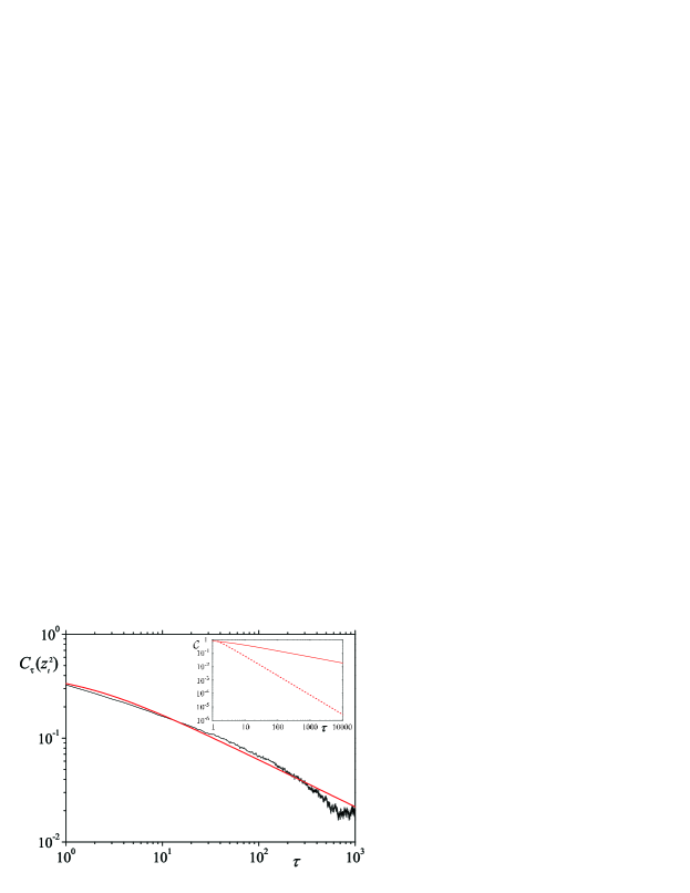
Figure 1: The black line presents the numerical evaluation of the $z_{t}^{2}$ autocorrelation function vs the lag $\tau$ and the red line $\mathcal{C}_{2}\left(\tau\right)$ from Eq. (20) for parameters $\left\{0.5,b=b_{SP},q_{m}=q_{SP}\right\}$. The inset depicts the way $\mathcal{C}_{1}\left(\tau\right)$ (dotted line) and $\mathcal{C}_{2}\left(\tau\right)$ (full line) decay. As it can be seen, $\mathcal{C}_{1}\left(\tau\right)$ decays much faster than $\mathcal{C}_{2}\left(\tau\right)$ which is the major responsible for $C_{\tau}\left(z_{t}^{2}\right)$ behaviour for large $\tau$.

and $\lambda=q_{c}^{-1}$. A simple inspection shows that $\mathcal{C}_{2}\left(\tau\right)$ decays much slower than $\mathcal{C}_{1}\left(\tau\right)$, hence the asymptotic form of $\left\langle z_{t}^{2}\,z_{t^{\prime}}^{2}\right\rangle$ is dominated by $\mathcal{C}_{2}\left(\tau\right)$ as it is illustrated in the inset of Fig. 1. In Fig. 1, we bring face to face Eq. (20) and the autocorrelation function of $z_{t}^{2}$ from numerical simulation using the parameters applied to reproduce $SP500$ returns previously determined, namely $\left\{a,b=b_{SP},q_{m}=q_{SP}\right\}=\left\{0.5,0.99635,1.6875\right\}$.

From all these equations we are able to conjecture expressions which relate parameters $\left\{a,b,q_{m}\right\}$ with the form of the distribution for the case where $\left\langle z_{t}^{4}\right\rangle$ is finite. In this way, we can use the ansatz that the distribution of this dynamical model is associated with a $q$-Gaussian (or Student-$t$) distribution ,

$$p\left(z\right)=\mathcal{A\,}\exp_{q}\left[-\mathcal{B}\,z^{2}\right],\qquad\left(q<3\right),$$ (22)

with $\mathcal{B}=\left[\bar{\sigma}_{q}^{2}\left(3-q\right)\right]^{-1}$, where,

$$\bar{\sigma}_{q}^{2}\equiv\int z^{2}\left[p\left(z\right)\right]^{q}dz/\int\left[p\left(z\right)\right]^{q}dz,$$

is the $q$-generalised second order moment [13], and $\mathcal{A}$ is the normalisation constant. This assumption is based on the same type of arguments used in [27] and whose accuracy we verify later on (see Sec. 3). For $q<5/3$, $\bar{\sigma}_{q}^{2}$ relates to the usual variance according to $\bar{\sigma}_{q}^{2}\left(3-q\right)=\bar{\sigma}^{2}\left(5-3\,q\right)$.

From Eqs. (13), (17), (19), and (20) we can write,

$$\begin{array}[]{cc}\left\langle z_{t}^{4}\right\rangle=&a^{2}\left\langle\omega_{t}^{4}\right\rangle+2a\,b\,\left\langle z_{t}^{2}\right\rangle\left\langle\omega_{t}^{4}\right\rangle+b^{2}\left\langle z_{t}^{4}\right\rangle\left\langle\omega_{t}^{4}\right\rangle\frac{\left(2-q_{m}\right)^{2}}{3-q_{m}}\\ &\\ &+b^{2}\left\langle\omega_{t}^{4}\right\rangle\left[a^{2}\left\langle\omega_{t}^{2}\right\rangle^{2}+2\,a\,b\,\left\langle z_{t}^{2}\right\rangle\,\left\langle\omega_{t}^{2}\right\rangle^{2}+2\mathcal{K}\right].\end{array}$$ (23)

where $\mathcal{K}$ represents terms like,

$$\int_{0}^{t}\int_{0}^{t}\exp_{q_{m}}\left[x-t\right]\exp_{q_{m}}\left[x+\tau-t\right]\left[\mathcal{C}_{1}\left(\tau\right)+\mathcal{C}_{2}\left(\tau\right)\right]\,d\tau\,dx,$$ (24)

which corresponds to a quite complex integration over $x$ of hypergeometric function special functions like $F_{2,1}\left[\tilde{a},\tilde{b};\tilde{c};x\right]$ and the Appell hypergeometric function [17] where $\tilde{a}$, $\tilde{b}$, and $\tilde{c}$ represent general values.

Taking into attention that for a $q$-Gaussian with $q<\frac{7}{5}$ its fourth moment is,

$$\left\langle z^{4}\right\rangle=3\left(\bar{\sigma}^{2}\right)^{2}\frac{3\,q-5}{5\,q-7},$$ (25)

we can obtain approximate relations between the parameters of the model and the parameters of the distribution. This is achieved when we equalise Eqs. (23) and (25), remembering the expression of the variance, Eq. (10), and the form of the autocorrelation function of $z_{t}^{2}$. This procedure is obviously important in parameter estimation. Therefore, from the decay of the $z_{t}^{2}$ autocorrelation function we can determine the value of $q_{m}$, and $a$ and $b$ from the equalisation we have just referred to together with Eq. (10).

3 Numerical considerations 

3.1 Stationary probability density functions

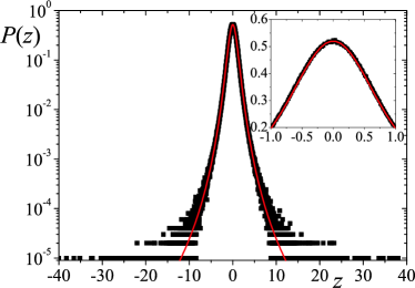
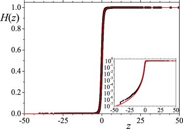
Figure 2: Upper panel: The symbols represent the probability density function $P\left(z\right)$ vs $z$ for parameters $q_{m}=1.5$ and $b=0.875$, and the line the best fit for a $q$-Gaussian with $q=1.385$ [on log-linear scale] and unitary standard deviation ($\chi^{2}=1.39\times 10^{-6}$ and $R^{2}=0.99987$). The inset is the same, but on linear-linear scale permitting the appraisal of the fitting in the central region. Lower panel: The symbols are for the empirical cumulative distribution function $H\left(z\right)$ vs $z$ for the same parameters and the line the CDF of a $q$-Gaussian with $q=1.385$ and unitary standard deviation ($D_{KS}=0.00457$). The inset is the same plot, but on a log-linear scale.

We firstly recover the results previously presented for the adjustment of $P\left(z\right)$ with $q$-Gaussians. As mentioned in [7] the adjustment is striking (diagrams of $q$ as a function of $b$ and $q_{m}$ are presented in Figure 1 of that reference). Using the method of $\chi^{2}$ minimisation, we have obtained for the same cases previously studied average values of $\chi^{2}=1.1\times 10^{-6}$ (per degree of freedom) and $R^{2}=0.99990$. In Fig. 2, we present an example for which it is possible to assent the accuracy of the fitting not only in the tails, but in the peak of the PDF as well. We have performed further analysis using the cumulative distribution function (CDF) and the Kolmogorov-Smirnov Distance, $D_{KS}$,

$$D_{KS}=\max\left|H\left(z\right)-H_{0}\left(z\right)\right|,$$ (26)

where $H\left(z\right)$ is the empirical CDF obtained from numerical evaluation of the model and $H_{0}\left(z\right)$ is the testing probability density function,

$$H_{0}\left(z\right)=\int_{-\infty}^{z}\mathcal{A\,}\exp_{q}\left[-\mathcal{B}\,x^{2}\right]\,dx.$$ (27)

The average $D_{KS}$ value obtained for the same cases plotted in Figure 1 of the prior work is equal to $4.25\times 10^{-3}$. Such values allow us to rely on the null hypothesis [19],

$$P\left(z\right)=p\left(z\right)=\mathcal{A\,}\exp_{q}\left[-\mathcal{B\,}z^{2}\right].$$ (28)

Based on the acceptance of the null hypothesis (28) we are able to introduce some insight into the distribution of $\sigma^{2}$, $p_{\sigma}\left(\sigma^{2}\right)$. Firstly, we carry out the following change of variables,

$$\left\{\begin{array}[]{c}\breve{z}_{t}=\ln\,z_{t}^{2}\\ \breve{\sigma}_{t}=\ln\,\sigma_{t}^{2}\\ \breve{\omega}_{t}=\ln\,\omega_{t}^{2}\end{array}\right.,$$ (29)

so that Eq. (1) turns into,

$$\breve{z}_{t}=\breve{\sigma}_{t}+\breve{\omega}_{t}.$$ (30)

In probability space, regarding that $\breve{\sigma}_{t}$ and $\breve{\omega}_{t}$ are independent, we have,

$$p\left(\breve{z}\right)=\int_{-\infty}^{\infty}P_{\breve{\sigma}}\left(\breve{\sigma}\right)\,P_{\breve{\omega}}\left(\breve{z}-\breve{\sigma}\right)\,d\breve{\sigma}.$$ (31)

We can now apply the convolution theorem. Being $p\left(\breve{z}_{t}\right)$, the probability of $\breve{z}_{t}$, according to such a theorem,

$$p\left(\breve{z}_{t}\right)=\mathcal{F}^{-1}\left[\check{P}_{\breve{\sigma}}\left(k\right)\check{P}_{\breve{\omega}}\left(k\right)\right],$$ (32)

where

$$\check{P}_{x}\left(k\right)=\frac{1}{\sqrt{2\,\pi}}\int f\left(x\right)\exp\left[i\,k\,x\right]\,dx\equiv\mathcal{F}\left[f\left(x\right)\right],$$ (33)

and $\mathcal{F}^{-1}\left[f_{x}\left(k\right)\right]=$ $\frac{1}{\sqrt{2\,\pi}}\int f_{x}\left(k\right)\exp\left[-i\,k\,x\right]\,dx=f\left(x\right)$ is the inverse Fourier Transform. Since we respectively know and postulate the form of $p\left(\omega\right)$ and $p\left(z\right)$, we can write down,

$$\begin{array}[]{c}p\left(\breve{\omega}\right)=\frac{1}{\sqrt{2\,\pi}}\exp\left[\frac{\breve{\omega}}{2}-\frac{e^{\breve{\omega}}}{2}\right],\\ \\ p\left(\breve{z}\right)=\mathcal{A\,}\exp_{q}\left[-\mathcal{B}\,e^{\,\breve{z}}\right]\exp\left[\frac{\breve{z}}{2}\right],\end{array}$$ (34)

($\mathcal{B=B}\left(\bar{\sigma}=1\right)$), yielding the respective Fourier Transforms [20],

$$\begin{array}[]{c}\check{P}_{\breve{\omega}}\left(k\right)=\frac{2^{i\,k-\frac{1}{2}}}{\pi}\Gamma\left[\frac{1}{2}+i\,k\right],\\ \\ \begin{array}[]{cc}\check{P}_{\breve{z}}\left(k\right)=&\frac{1}{\sqrt{2\pi}}\mathcal{A}\left\{\left(-1\right)^{-Q}\left(\mathcal{B\,}q-\mathcal{B}\right)^{\frac{1}{1-q}-Q}B\left[\frac{1}{\mathcal{B}-\mathcal{B\,}q},Q,\frac{2-q}{q-1}\right]\right.+\\ &\\ &\left.\Gamma\left[\frac{1}{2}+i\,k\right]\tilde{F}_{2,1}\left[\frac{1}{q-1},\frac{1}{2}+ik,\frac{3}{2}+ik,\mathcal{B}-\mathcal{B\,}q\right]\right\}.\end{array}\end{array}$$ (35)

where $Q=\frac{1}{1-q}+\frac{1}{2}+ik$, $B\left[\ldots\right]$ is the Beta function, and $\tilde{F}_{2,1}\left[\ldots\right]$ is the regularised hypergeometric function [17]. Applying Eq. (35) in Eq. (32) we can compute the distribution of $\breve{\sigma}$ (easily related to $p_{\sigma}\left(\sigma\right)$),

$$P_{\breve{\sigma}}\left(\breve{\sigma}\right)=\mathcal{F}^{-1}\left[\frac{\check{P}_{\breve{z}}\left(k\right)}{\check{P}_{\breve{\omega}}\left(k\right)}\right],$$ (36)

From a laborious and tricky calculation, using properties of $\tilde{F}_{2,1}\left[\ldots\right]$ (see [18] and related properties), it can be verified $P_{\breve{\sigma}}\left(\breve{\sigma}\right)$ cooresponds to,

$$\check{P}_{\breve{\sigma}}\left(k\right)=\frac{\Gamma\left[\theta-i\,k\right]}{\left(2\beta\right)^{i\,k}\Gamma\left[c\right]}.$$ (37)

Therefore, $\sigma^{2}$ follows an inverse Gamma distribution,

$$p_{\sigma}\left(\sigma^{2}\right)=\frac{1}{\left(2\,\theta\right)^{c}\,\Gamma\left[c\right]}\left(\sigma^{2}\right)^{-1-c}\exp\left[-\frac{1}{2\,\theta\,\sigma^{2}}\right],$$ (38)

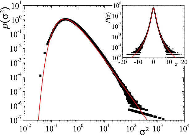
Figure 3: The black symbols represent $p_{\sigma}\left(\sigma^{2}\right)$ vs $\sigma^{2}$ [on log-log scale] obtained by numerical evaluation of the process with $q_{m}=q_{SP}$ and $b=b_{SP}$ yielding a $q$-Gaussian distribution with $q=1.465$ ($\chi^{2}=1.6\times 10^{-6}$) shown in the inset [on log-linear scale]. The red line in the main plot is the representation of the inverted Gamma distribution with $c=1.648\ldots$ and $\theta=0.770\ldots$ ($\chi^{2}=6.1\times 10^{-4}$).

where $c=\frac{3-q}{2\,q-2}$ and $\theta=\frac{q-1}{\bar{\sigma}^{2}\left(5-3\,q\right)}$. This result attests the validity of the superstatistical approach to the problem of heteroskedasticity. It is worth mentioning that superstatistics [21] represents the long-term statistics in systems with fluctuations in some characteristic intensive parameter of the problem like the dissipation rate in Lagragian turbulent fluids [22] or the standard deviation like in the subject matter of heteroskedasticity. For the values of $q_{SP}$ and $b_{SP}$, with have obtained random variables $z_{t}$ associated with a $\left(q=1.465\right)$-Gaussian. This yields $c_{SP}=1.648\ldots$ and $\theta_{SP}=0.770\ldots$, which have been applied in Fig. 3 to fit $p_{\sigma}\left(\sigma^{2}\right)$ obtained by numerical procedures. In that plot, it is visible that numerical and analytical curves are in proximity.

3.2 Dependence degree

The degree that the elements of a time series are tied-in is not completely expressed by the correlation function in the majority of the cases. In fact, regarding its intimate relation with the covariance, the correlation function is only a measure of linear dependences. Aiming to assess non-linear dependences, information measures have been widely applied [23]. In our case, we use a non-extensive generalisation of Kullback-Leibler information measure [24, 25],

$$I_{q}\equiv-\sum_{t}p\left(z_{t}^{2},z_{t+\tau}^{2}\right)\frac{\left[\frac{p^{\prime}\left(z_{t}^{2},z_{t+\tau}^{2}\right)}{p\left(z_{t}^{2},z_{t+\tau}^{2}\right)}\right]^{1-q}-1}{1-q},$$ (39)

where $p^{\prime}\left(z_{t}^{2},z_{t+\tau}^{2}\right)=p\left(z_{t}^{2}\right)p\left(z_{t+\tau}^{2}\right)=\left[p\left(z^{2}\right)\right]^{2}$ (assuming stationarity), which has been able to provide a set of interesting results with respect to dependence problems [26]. The quantification of the dependence degree is made through a value, $q^{op}$, which corresponds to the inflexion point of the normalised version of $I_{q}$,

$$R_{q}\equiv\frac{I_{q}}{I_{q}^{\max}},$$ (40)

where $I_{q}^{\max}$ is the value of $I_{q}$ when variables $z\left(t\right)$ and $z\left(t+\tau\right)$ present a biunivocal dependence (see full expression in Ref. [25]).

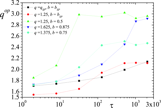
Figure 5: Values of $q^{op}$ vs time lag $\tau$ for the pairs $\left\{q_{m}=q_{SP},b=b_{SP}\right\}$ as indicated in the figure. The dotted lines are merely presented as a guide to the eye.

For infinite signals it can be shown that, when the variables are completely independent $q^{op}=\infty$, whereas $q^{op}=0$ when variables are one-to-one dependent. For finite systems, there is a noise level, $q_{n}^{op}$, which is achieved after a finite time lag $\tau$. Typical curves of $R_{q}$ are depicted in Fig. 5 for $q_{m}=q_{SP}$ and $b=b_{SP}$.

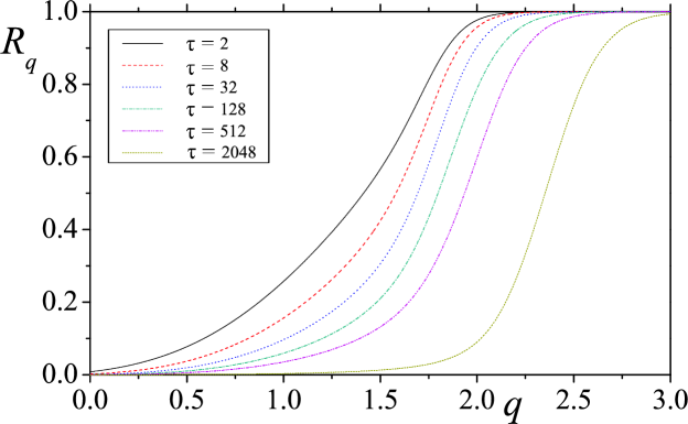
Figure 4: Normalised generalised mutual entropy $I_{q}$ vs $q$ for parameters $\left\{q_{m}=q_{SP},b=b_{SP}\right\}$ and values of the lag presented in the figure.

In what follows, we present results obtained from numerical evaluation of $R_{q}$ for different values of $\tau$. As expected, dependence relies on the balance between the extension of memory, which is given by $q_{m}$ and the weight of effective past value, $\tilde{z}_{t-1}$, on $\sigma_{t}$. Firstly, let us compare cases $\left\{q_{m}=q_{SP},b=b_{SP}\right\}$ and $\left\{q_{m}=1.25,b=b_{SP}\right\}$, as an example of what happens when we fix $b$ as a constant (see Fig. 4). Dependence is obviously long-lasting in the former case, in the sense that it takes longer to attain $q_{n}^{op}$, but for small values of $\tau$, the latter has presented higher levels of dependence. This has to do that $\mathcal{K}\left(t^{\prime}\right)$ is normalised and that implies the intersection of the curves for different values of $q_{m}$ at some value of $t^{\prime}$. Alternatively, when $q_{m}$ decreases, the recent values of $z_{t}$ have more influence on $\tilde{z}_{t-1}$ than past values. When the value of $q_{m}$ is kept constant, we have verified that smaller values of $b$ lead to a faster approach to noise value $q_{n}^{op}$. In a previous work on $GARCH\left(1,1\right)\leavevmode\nobreak\$ [27], we have verified that variables approximately associated with the same distribution present the same level of dependence independently of the pair $\left(b,c\right)$ chosen. In this case, recurring to cases $\left\{q_{m}=1.375,b=0.75\right\}$ and $\left\{q_{m}=1.625,b=0.875\right\}$, we have noticed that the curves present very close values for small lags, but they fall apart for $\tau>10$, revealing a more intricate relation between $q$, $q_{m}$, and $b$ than in $GARCH\left(1,1\right)$. Additionally, comparing dependence and correlation, we have verified that the decay is faster for the latter. Specifically, taking into account noise values of $q^{op}$ and $C_{\tau}\left(z_{t}^{2}\right)$, it is verifiable that $q^{op}$ takes longer to achieve $q_{n}^{op}$ than $C_{\tau}\left(z_{t}^{2}\right)$ takes to reach $C_{n}\left(z_{t}^{2}\right)$.

3.3 First-Passage Times

First-passage studies in stochastic processes are of considerable interest. Not only from the scientific point of view [28] (it is useful in the approximate calculation of the lifetimes of the problems/systems) as well as from a practical perspective, since they can be applied to quantify the extent of reliability of forecasting procedures, e.g., in meteorology or finance [1, 29, 30]. In what it is next to come, we have analysed the probability of $z_{t}^{2}\in S_{i}=\left[a,b\right)$ and $z_{t+T}^{2}\in S_{i}$. We have divided $z_{t}^{2}$ domain into five different intervals. Explicitly:

• $S_{1}$: $z_{t}^{2}\leq 1$;

• $S_{2}$: $1<$ $z_{t}^{2}\leq 2$;

• $S_{3}$: $2<$ $z_{t}^{2}\leq 5$;

• $S_{4}$: $5<$ $z_{t}^{2}\leq 10$;

• $S_{5}$: $z_{t}^{2}>10$.

Analysing the probability density functions we have verified that the simplest expression which enables a numerical description of first-passage inverse cumulative probability distribution, $\mathcal{D}\left(\mathfrak{t}\right)$, is a linear composition of a asymptotic power-law (or a $\nu$-exponential) with a stretched exponential,

$$\mathcal{D}\left(\mathfrak{t}\right)=\epsilon\left[1+\left(\nu-1\right)\frac{\mathfrak{t}}{\mathfrak{T}_{1}}\right]^{\frac{1}{1-\nu}}+\left(1-\epsilon\right)\exp\left[-\left(\frac{\mathfrak{t}}{\mathfrak{T}_{2}}\right)^{\phi}\right].$$ (41)

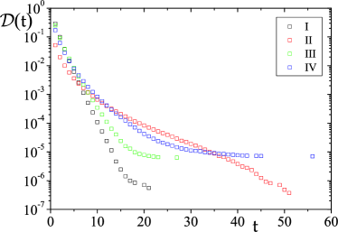
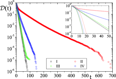
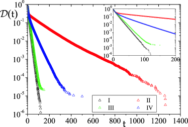
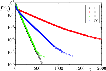
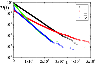
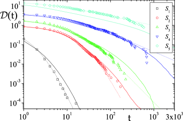
Figure 6: Inverse cumulative distribution $\mathcal{D}\left(\mathfrak{t}\right)$ of the first-passage times vs$\mathfrak{t}$ for the sets of parameters mentioned in the text. Upper panels: region $S_{1}$ (left) and $S_{2}$ (right); Middle panels: region $S_{3}$ (left) and $S_{4}$ (right); Lower left panel: region $S_{5}$ (left). For the regions $S_{2}-S_{5}$, the exponential decay is evident. Lower right panel: Inverse cumulative distribution $\mathcal{D}\left(\mathfrak{t}\right)$ of the first-passage times vs $\mathfrak{t}$ for squared daily price fluctuations of $SP500$ (symbols) with the best fit represented by the dotted lines. The full lines are obtained from the model with parameters $q_{m}=q_{SP}$ and $b=b_{SP}$. The non-exponential behaviour is clear in this latter case. The curves of the $S_{3}-S_{5}$ regions are shifted by a factor of 2, 4, and 16, respectively.

Curves of some analysed cases are presented in Fig. 6 and fitting parameters in Tab. 1. The cases we present are: $I$-$\left\{q_{m}=q_{SP},b=0.5\right\}$, $II$-$\left\{q_{m}=1.25,b=b_{SP}\right\}$, $III$-$\left\{q_{m}=1.25,b=0.5\right\}$, $IV$-$\left\{q_{m}=1.5,b=0.875\right\}$.

From the Fig. 6 we have verified that, excepting region $S_{1}$, all curves of $\mathcal{D}\left(\mathfrak{t}\right)$ exhibit a decay closely exponential ($\nu=1$). For region $S_{1}$, as we increase the non-Gaussianity of $p(z_{t})$, we have observed that both of the values of $\epsilon$ and $\nu$ approach one. Comparing the remaining curves, we have verified that, for every region $S_{2}-S_{5}$, the set of parameters which provides higher degree of non-Gaussianity has the larger characteristic times $\mathfrak{T}$. Keeping the memory parameter $q_{m}$ constant, we have observed that the higher $b$, the higher $\mathfrak{T}$ is. An inverse dependence is found when we have fixed $b$ and let $q_{m}$ vary. In other words, smaller values of $q_{m}$ (which enhance broader distributions) have larger values of $\mathfrak{T}$. We have also verified that the first-passage times are not Poisson distributed as it is straightforwardly verified in $S_{2}$ plots. Looking at the values of squared daily index fluctuations of $SP500$, we have verified that they present an asymptotic power-law behaviour for $\mathcal{D}\left(\mathfrak{t}\right)$ ($\epsilon=1$, $\nu>1$) (fitting parameters shown in Tab. 2). Comparing the results of the model with empirical results from $SP500$ time series, we have observed that the model provides an overall reasonable description of first-passage times with curves almost superposing for $S_{2}-S_{4}$ regions. For $S_{1}$ and $S_{5}$ regions curves present similar exponents, but different values of $\mathfrak{T}$. It is worth remembering that we can improve the results by considering some characteristic time in $\mathcal{K}\left(t\right)$ equation. Taking into account the $\nu$ exponents obtained for the adjustment of $SP500$ first-passage times, we verify that larger and smaller $\nu$- exponents are quite different. Such a strong gap invalidates, at a daily scale, the collapse (existence of a single exponent) of $\mathcal{D}\left(\mathfrak{t}\right)$ curves proposed for high-frequency data [29].

3.4 Multiscaling properties

Multiscaling has been the focus of several studies in the field of complexity [31], particularly regarding applications to finance [32][33][34]. If in many works multiscaling (multifractal) properties of price fluctuations are presented, other studies have put those multiscaling properties into questioning [35]. In this section, we analyse mainly multifractal properties of $z_{t}$ and $z_{t}^{2}$. To this aim, we define a generic variable

$$Z_{t}^{\left(2\right)}\left(T\right)\equiv\sum_{i=1}^{T}z_{t+i-1}^{\left(2\right)}.$$ (42)

From it, we compute,

$$\Omega_{h}\left(T\right)\equiv\left\langle\left|Z_{t}^{\left(2\right)}\left(T\right)-\left\langle Z_{t}^{\left(2\right)}\left(T\right)\right\rangle\right|^{h}\right\rangle.$$ (43)

If there is multiscaling, then the following scaling property is observed,

$$\Omega_{h}\left(T\right)\propto T^{\eta\left(h\right)}.$$ (44)

The computation of $\Omega_{h}\left(T\right)$ has been made using the well-known MF-DFA procedure [36].

For the case of $z_{t}$, the multiscaling can be easily and analytically explained. The multiscaling properties of a time series can emerge twyfold: from memory and from non-Gaussianity. Since, by definition, the heteroskedastic process we present is uncorrelated, then the only contribution to multiscaling comes from the non-Gaussian character of probability density functions. In this way, time series $\left\{z_{t}\right\}$ is not a multifractal, but a bifractal instead [36]. Therefore, the $\eta\left(h\right)$ curve is defined as follows,

$$\eta\left(h\right)=\left\{\begin{array}[]{ccc}h\frac{q-1}{3-q}&\mathrm{for}&h<\frac{3-q}{q-1}\\ 0&\mathrm{for}&h>\frac{3-q}{q-1}\end{array}\right..$$ (45)

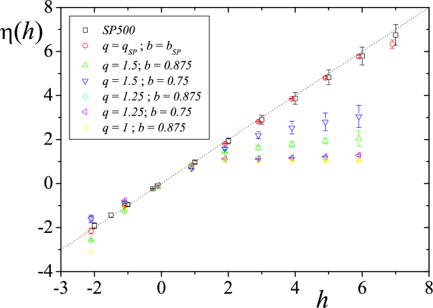
Figure 7: Multiscaling exponents $\eta$ vs moments $h$ of the values presented in the plot. The dashed line is $\eta=h$.

With respect to $Z_{t}^{2}$ contrastive properties of $Z_{t}$ are found. The results obtained from $SP500$ time series and the surrogate data have enabled us to verify that the model is adequate to reproduce the scaling properties of $Z_{t}^{2}$ which are basically linear according to $\eta\left(h\right)=h$. For a constant $b$ value, we have observed that higher correlations, introduced by increasing the value of $q_{m}$ turn multiscaling properties weaker. In other words, $\eta_{z^{2}}\left(h\right)$ approaches the straight line $\eta_{z^{2}}\left(h\right)=h$. Similar qualitative results have been presented for traded value where long-lasting correlations dominate specially for highly liquid equities [34]. Freezing memory parameter, $q_{m}$, we have verified similar results, i.e., increasing the value of $b$, we increase the tails in $z^{2}_{t}$ forcing the multiscaling curve to divert (even more) from the straight line $\eta=h$. The same effect is obtained when memory is shortened by reducing the value of $q_{m}$. By this we mean that, when memory decays faster we have a detour from the straight line $\eta=h$ and an approximation to a bifractal behaviour because of the asymptotic power-law behaviour. This reflects the fact that the dynamical and statistical properties of our system strongly depend on the “force relation” between $b$ and $q_{m}$. Some results from which these observations can be confirmed are shown in Fig. 7.

4 Asymmetric variance model 

In several systems it has been verified that the correlation function between the observable and its instantaneous variance exhibits an anticorrelation dependence. For example, this occurs in the case of financial markets, when the correlation between past price fluctuations and present volatilities is measured. The shape of the curve copes with the so called leverage effect [37, 38]. This feature is intimately related to the risk aversion phenomenon, i.e., falls in price turn the market more volatile than price rises. In order to reproduce this characteristic we introduce a small change in Eq. (6), specifically,

$$\tilde{z}_{t-1}^{2}=\sum\limits_{i=t_{0}}^{t-1}\mathcal{K}\left(i-t+1\right)\,\left[z_{i}\left(1-c\,z_{i}\right)\right]^{2},$$ (46)

where $c\geq 0$. It is worth stressing that this modification does not introduce any skewness in the distribution $P\left(z\right)$ which is still symmetric. It only acts on how positive and negative values of $z_{t}$, with the same magnitude, influence $\tilde{z}_{t}^{2}$ by different amounts.

Using Eqs. (5) and (46) in Eq. (1) and expanding it up to first order we have

$$z_{t}=\left\{\sqrt{a}+\frac{b}{2}\sum\limits_{i=t_{0}}^{t-1}\mathcal{K}\left(i-t+1\right)\left[z_{i}^{2}-2\,c\,z_{i}^{3}+c^{2}z_{i}^{4}\right]+\ldots\right\}\,\omega_{t}.$$ (47)

Computing $z_{t}\,z_{t+\tau}^{2}$ the only terms which do not vanish after averaging are

$$\mathcal{T}_{1}=-2\sqrt{a}\,b\,c\sum\limits_{i=t_{0}}^{t-1+\tau}\mathcal{K}\left(i-\left(t-1+\tau\right)\right)\,z_{i}^{3}\,\omega_{t}\,\omega_{t+\tau}^{2},$$ (48)

and

$$\begin{array}[]{cc}\mathcal{T}_{2}=&-2\,b\,c^{3}\sum\limits_{i=t_{0}}^{t-1+\tau}\sum\limits_{j=t_{0}}^{t-1}\mathcal{K}\left(i-\left(t-1+\tau\right)\right)\mathcal{K}\left(j-t+1\right)\times\\ &\\ &z_{i}^{3}\,z_{j}^{4}\,\omega_{t}\,\omega_{t+\tau}^{2}.\end{array}\,$$ (49)

Performing averages and considering stationarity we have in the continuous limit,

$$\begin{array}[]{cc}\left\langle\mathcal{T}_{1}\right\rangle=&--6\sqrt{a}\,b\,c\int_{0}^{t+\tau}\mathcal{K}\left(x-\left(t+\tau\right)\right)\times\\ &\\ &\left\langle z_{t}^{2}\right\rangle\,\left\langle\sigma_{t}\right\rangle\,\left\langle\omega_{t}^{2}\right\rangle\,\delta\left(x-t\right)\,dx,\end{array}\,$$ (50)

which gives,

$$\left\langle\mathcal{T}_{1}\right\rangle\sim-\exp_{q_{m}}\left[-\tau\right].$$ (51)

$$\begin{array}[]{cc}\mathcal{T}_{2}=&-2\,b\,c^{3}\left\{\int_{0}^{t}\mathcal{K}\left(x-\left(t+\tau\right)\right)\mathcal{K}\left(x-t\right)\,z_{x}^{7}\,\omega_{t}\,\omega_{t+\tau}^{2}\,dx+\right.\\ &\\ &2\int_{0}^{t}\int_{x}^{t}\mathcal{K}\left(x-\left(t+\tau\right)\right)\mathcal{K}\left(y-t\right)z_{x}^{3}z_{y}^{4}\,\omega_{t}\,\omega_{t+\tau}^{2}\,dx\,dy+\\ &\\ &\left.\int_{t}^{t+\tau}\int_{0}^{t}\mathcal{K}\left(x-\left(t+\tau\right)\right)\mathcal{K}\left(y-t\right)z_{x}^{3}z_{y}^{4}\,\omega_{t}\,\omega_{t+\tau}^{2}\,dx\,dy\right\}.\end{array}$$ (52)

Averaging, only the first integral has a non-null contribution yielding,

$$\left\langle\mathcal{T}_{2}\right\rangle=-2\,b\,c^{3}\left(2-q_{m}\right)^{2}\exp_{q_{m}}\left[-\tau\right]\left\langle z_{t}^{6}\right\rangle\left\langle\sigma_{t}\right\rangle\left\langle\omega_{t}^{2}\right\rangle.$$ (53)

It is not hard to show that

$$\begin{array}[]{cc}\left\langle z_{x}^{3}z_{y}^{4}\,\omega_{t}\right\rangle=&5\,\,\delta\left(x-t\right)\left\langle\sigma_{t}\right\rangle\left\langle z_{t}^{2}\right\rangle\left\langle z_{t}^{4}\right\rangle+\\ &\\ &24\,\delta\left(y-t\right)\delta\left(x-y\right)\left\langle\sigma_{t}\right\rangle\left\langle\sigma_{t}^{2}\right\rangle\left\langle z_{t}^{2}\right\rangle^{2}+\\ &\\ &72\,\delta\left(x-t\right)\left[\delta\left(x-y\right)\right]^{2}\left\langle\sigma_{t}\right\rangle\left\langle\sigma_{t}^{2}\right\rangle\left\langle z_{t}^{2}\right\rangle+\\ &\\ &12\,\delta\left(x-y\right)\left\langle\sigma_{t}\right\rangle\left\langle z_{x}^{2}z_{y}^{3}\omega_{t}\right\rangle+\\ &\\ &12\,\delta\left(y-t\right)\delta\left(x-y\right)\left\langle\sigma_{t}\right\rangle^{2}\left\langle z_{x}^{2}z_{y}^{2}\right\rangle.\end{array}$$ (54)

Inserting Eq. (54) in Eq. (52) the last two integrals give zero. Therefore, in the first approximation, the leverage function,

$$\mathcal{L}\equiv\frac{\left\langle z_{t}\,z_{t+\tau}^{2}\right\rangle}{\left\langle z_{t}^{2}\right\rangle^{2}},$$ (55)

goes as,

$$\mathcal{L}\sim\left\langle\mathcal{T}_{1}\right\rangle+\left\langle\mathcal{T}_{2}\right\rangle\sim-\exp_{q_{m}}\left[-\tau\right].$$ (56)

As it can be seen from Fig. 8, the approximation provides a satisfactory approximation of the numerical results. A precise description can obviously be obtained by considering higher-order (slowly decaying) terms which are obtained through a quite tedious computation that follows exactly the same lines we have just introduced.

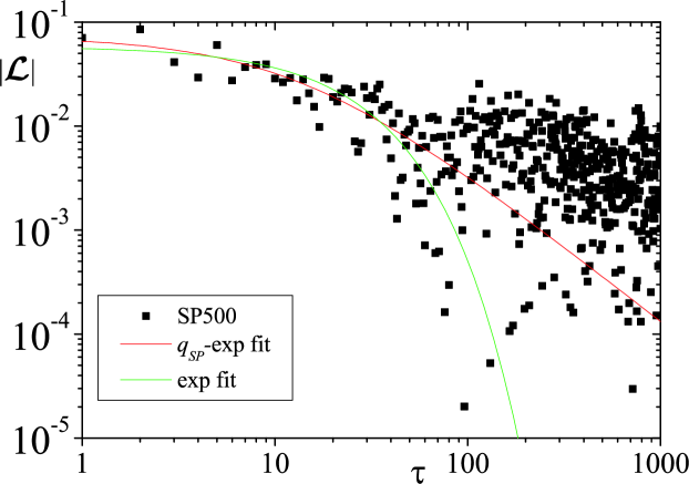
Figure 9: The symbols represent the absolute value of leverage $\mathcal{L}$ vs time lag $\tau$ for the daily index fluctuations of $SP500$ spanning the period mentioned above. The red line represents the fitting for a $q$-exponential function with $L_{0}=0.07$, $q=q_{SP}$ and $T=9$, and the green line a exponential fitting with $L_{0}=0.06$ and $T=20$ (fitting error values in the text).

The result above is in apparent contradiction with previous work in which an exponential dependence with $\tau$ is defended in lieu of an asymptotic power-law dependence. Nevertheless, in Fig. 9 we show the leverage function computed from the $SP500$ and numerical adjustments with function,

$$L\left(\tau\right)=-L_{0}\exp_{q_{m}}\left[-\frac{\tau}{T}\right],$$ (57)

with $q_{m}=q_{SP}$ and $q_{m}=1$. Computing the adjustment error, $\chi^{2}$ and $R^{2}$, we verify that both approaches present similar values for the numerical adjustment with $q=q_{SP}$ being scanty better. For $q=q_{SP}$, we have obtained $\chi^{2}=4\times 10^{-5}$ and $R^{2}=0.47$ and for the exponential adjustment $\chi^{2}=5\times 10^{-5}$ and $R^{2}=0.44$. From these results, we can affirm that our proposal is, at least, as good as the exponential decay scenario firstly introduced in Ref. [38]. It is also worth noting that, although this variation is asymmetric concerning the effects of the sign of variables $z_{t}$ on the evaluation of $\sigma_{t}^{2}$, the model is ineffective in reproducing the skewness of the distribution of price fluctuations. This owes to the fact that $\omega_{t}$ used up to now is symmetric thus, also annulling the asymmetry introduced by the Eq. (46). It is worth stressing that moments $\left\langle z_{t}^{n}\right\rangle$, for $n$ even, in this section are obviously different from the values presented in preceding sections.

5 Final remarks 

In this manuscript we have introduced further insight into a heteroskedastic process enclosed in the class of fractionally integrated $ARCH$ processes. This process is characterised by a memory of past values of the squared variable which decays according to an $q_{m}$-exponential. Despite of the fact that we were unable to provide an analytical proof, prevailing statistical testing has shown that $q$-Gaussian distributions properly describe the probability density function of the generated stochastic variable. Based on this fact, we have determined a form of the instantaneous variance, $\sigma^{2}$, probability density function which has yielded a inverse Gamma distribution like it happens in superstatistical models giving $q$-Gaussians as long-term distributions. Moreover, we have computed the first term of the correlation function, $C_{\tau}\left(z_{t}^{2}\right)$, which corresponds to a $q_{c}$-exponential. An analytical relation between $q_{m}$ and $q_{c}$ is presented. From these results, we are able to state that this dynamical system can actually be described within non-extensive statistical mechanics (NESM) framework by a triplet of $q$ values [39]. As a matter of fact, this process presents all the elements to be characterised, in $z_{t}^{2}$ variable, as a NESM process. Explicitly, besides presenting asymptotic power-law distributions which maximise non-additive entropy $S_{q}$ (as $z_{t}$), it has a slow decaying ($q_{c}$-exponential) auto-correlation function, and it exhibits multiscaling properties. Such properties have been advocated as primary features of systems that should be studied within NESM framework (for related literature see [40]) for a long time. Furthermore, we have verified that, for a sufficiently high level of memory the model presents a non-exponential distribution of first-passage times and strong levels of dependence measured from a generalisation of Kullback-Liebler mutual information. Though they have been applied in several other areas, in view of the fact that hetoskedastic processes have been introduced in a financial context, we have tested the model against daily index fluctuations of $SP500$. The results firstly presented, together with the results of this manuscript, show that this model, despite of its simplicity (it only has two parameters), is able to reproduce the most relevant and important properties, namely the probability density functions, the Hurst exponent, the autocorrelation functions, multiscaling, and first-passage time distribution (in a less good extend compared to previous). It is our belief that the same occurs with other time series presenting similar characteristics. Moreover, we have studied how the extension of the memory (tuned by $q_{m}$) and its weight, or alternatively, the weight of fluctuations in $\sigma_{t}^{2}$ (adjusted by $b$) have on the quantities. Still in the context of financial time series, we have introduced a slight modification which allows the reproduction of the leverage effect. Under these circumstances, we propose that the leverage is not described for an exponential function, but for a $q_{m}$-exponential function instead. When statistically tested, this proposal has emerged as good as the exponential description. It is well-known that many distributions obtained from complex systems present skweness which this model has not been able to capture because of the symmetrical nature of noise $\omega$ distribution. The use of other types of noise $\omega$, jointly with the modification presented in Sec. 4 might give rise to even more precise modelling.

Acknowledgements

SMDQ acknowledges C. Tsallis for several comments and discussions on matters related to this manuscript. This work benefited firstly from financial support from FCT/MCES (Portuguese agency) and infrastructural support from PRONEX/MCT (Brazilian agency) and in its later part from financial support from Marie Curie Fellowship Programme (European Union).

Figure 8: The symbols represent leverage $\mathcal{L}$ vs time lag $\tau$ of a processes using Eq. (46) with $q_{m}=1.65$, $b=0.95$ and $c=0.1$ obtained from a time series of $10^{6}$ elements. The red line is the best fit using Eq. (56) with $\mathcal{L}\left(\tau=0\right)=-0.39$ ($\chi^{2}=3\times 10^{-4}$).

Table 1: Table of the fitting parameters of region $S_{1}$using Eq. (41)

	$I$	$II$	$III$	$IV$
$\epsilon$	$0.388$	$0.004$	$0.414$	$0.334$
$\nu$	$1.09$	$1$	$1.17$	$1.17$
$\mathfrak{T}_{1}$	$0.648$	$2.23$	$0.541$	$0.951$
$\phi$	$0.894$	$0.394$	$0.792$	$0.762$
$\mathfrak{T}_{2}$	$0.867$	$0.001$	$0.757$	$0.27$
$\chi^{2}$	$5.1\times 10^{-9}$	$9.2\times 10^{-7}$	$2.6\times 10^{-6}$	$1.9\times 10^{-6}$

Table 2: Table of the fitting parameters of dily index fluctuation of $SP500$ region using Eq.(41).

	$S_{1}$	$S_{2}$	$S_{3}$	$S_{4}$	$S_{5}$
$\epsilon$	$1$	$1$	$1$	$1$	$1$
$\nu$	$1.17$	$1.21$	$1.43$	$2.03$	$3.03$
$\mathfrak{T}_{1}$	$1.85$	$0.14$	$0.157$	$0.101$	$0.143$
$R^{2}$	$0.999$	$0.999$	$0.998$	$0.998$	$0.993$
$\chi^{2}$	$5.4\times 10^{-7}$	$5\times 10^{-5}$	$5\times 10^{-5}$	$1\times 10^{-4}$	$3\times 10^{-4}$

References

- [1] J.-P. Bouchaud and M. Potters, Theory of Financial Risks: From Statistical Physics to Risk Management (Cambridge University Press, Cambridge, 2000); R.N. Mantegna and H.E. Stanley, An introduction to Econophysics: Correlations and Complexity in Finance (Cambridge University Press, Cambrigde, 1999); J. Voit, The Statistical Mechanics of Financial Markets (Springer-Verlag, Berlin, 2003); M. Dacorogna, R. Gençay, U. Müller, R. Olsen, and O. Pictet, An Introduction to High-Frequency Finance (Academic Press, London, 2001)
- [2] S. Campbell and F.X. Diebold, J. Am. Stat. Ass. 100, 6 (2005)
- [3] J.D. Martin-Guerrero, G. Camps-Valls, E.Soria-Olivas, A.J. Serrano-Lopez, J.J. Perez-Ruixo and N.V. Jimenez-Torres, IEEE Trans. Biomed. Eng. 50, 1136 (2003)
- [4] P. Gronke J. Brehm, Elect. Stud. 21, 425 (2002)
- [5] T.G. Andersen, T. Bollerslev, P.F. Christoffersen and F.X. Diebold, Volatility Forecasting, PIER working paper 05-011, 2005
- [6] R.F. Engle, Econometrica 50, 987 (1982)
- [7] S. M. Duarte Queirós, Europhys. Lett. 80, 30005 (2007)
- [8] B. Pobodnik, P.Ch. Ivanov, Y. Lee, A. Cheesa, and H.E. Stanley, Europhys. Lett. 50, 711 (2000); S.M. Duarte Queirós and C. Tsallis, Europhys. Lett. 69, 893 (2005)
- [9] M. Porto and H.E. Roman, Phys. Rev. E 63, 036128 (2001)
- [10] T. Bollerslev, R.Y. Chou, and K.F. Kroner, J. Econometrics 52, 5 (1992); T.G. Andersen, T. Bollerslev, and F.X. Diebold, in Handbook of Financial Econometrics, edited by Y. Aït-Sahalia (Elsevier, Amsterdam, 2006)
- [11] Z. Zing, C.W.J. Granger, and R.F. Engle, J. Emp. Fin. 1, 83 (1983)
- [12] C. Gourieroux and A. Montfort, Statistics and Econometric Models, (Cambridge University Press, Cambridge, 1996)
- [13] C. Tsallis, J. Stat. Phys. 52 , 479 (1988); C. Tsallis, Braz. J. Phys. 29, 1 (1999)
- [14] C.W.J. Granger, and Z. Ding, J. Econometrics 73, 61 (1996); H.E. Roman and M. Porto, Int. J. Mod. Phys. C (to be published)
- [15] C. Dose, M. Porto, and H.E. Roman, Phys. Rev. E 67, 067103 (2003)
- [16] G.M. Schütz and S. Trimper, Phys. Rev. E 70, 045101(R) (2004)
- [17] http://functions.wolfram.com
- [18] functions.wolfram.com/07.24.26.0272.01
- [19] D.C. Boes, F.A. Graybill, and A.M. Mood, Introduction to the Theory of Statistics, 3rd edn. (McGraw-Hill, New York, 1974); H.R. Neave, Statistics Tables for mathematicians, engineers, economists and the behavioural and management sciences (Routledge, London, 1999)
- [20] I.S. Gradshteyn, I.M. Ryzhik, Tables of integrals, series and products (Academic Press, London, 1965)
- [21] C. Beck, E.G.D. Cohen, Physica A 322, 267 (2003)
- [22] A.M. Reynolds, N. Mordant, A.M. Crawford, and E. Bodenschatz, New J. Phys. 7, 58 (2005); C. Beck, Phys. Rev. Lett. 98, 064502 (2007)
- [23] K. Hlaváčková-Schlinder, M. Paruš, M. Vejmelka, J. Bhattacharya, Phys. Rep. 441, 1 (2007)
- [24] C. Tsallis, Phys. Rev. E 58, 1442 (1998)
- [25] L. Borland, A.R. Plastino and C. Tsallis, J. Math. Phys. 39, 6490 (1998) [Errata: J. Math. Phys. 40, 2196 (1999)]
- [26] S.M. Duarte Queirós, Quantitatit. Finance 5, 475 (2005); M. Portesi, F. Pennini, and A. Plastino, Physica A 373, 273 (2007); S.M. Duarte Queirós, e-print arXiv:0805.2254 [cond-mat.stat-mech] (preprint, 2008)
- [27] S.M.D. Queirós and C. Tsallis, Eur. Phys. J. B 48, 139 (2005)
- [28] H. Risken, The Fokker-Planck Equation: Methods of Solution and Applications (Springer-Verlag, Berlin, 1989)
- [29] F. Wang, P. Weber, K. Yamasaki, S. Havlin, and H.E. Stanley, Eur. Phys. J. B 55, 123 (2007); E. Scalas, Chaos Solitons & Fractals (to be published)
- [30] B. Hoskins, in Predictability of Wheather and Climate, edited by T. Palmer and R. Hagedorn (Cambridge University Press, Cambridge, 2006)
- [31] B.B. Mandelbrot, The Fractal Geometry of Nature (W.H. Freeman & Co., San Francisco - CA, 1983); J. Feder, Fractals (Plenum, New York, 1988)
- [32] B.B. Mandelbrot, Fractals and Scaling in Finance (Springer, New York, 1997)
- [33] A. Admati and P. Pfleiderer, Rev. Financial Studies 1 (1988); A. Arnéodo, J.-F. Muzy, and D. Sornette, Eur. Phys. J. B 2, 277 (1998), K. Ivanova and M. Ausloos, Eur. Phys. J. 8 (1999) 665; B. Pochart and J.P. Bouchaud, e-print arXiv:cond-mat/0204047 (preprint, 2002); T. Di Matteo, Quantit. Finance 7, 21 (2007); P. Oświȩcimka, J. Kwapień, and S. Drożdż, Phys.Rev. E 74, 016103 (2006) ; L.G. Moyano, J. de Souza, and S.M. Duarte Queirós, Physica A 371, 118 (2006); F. Wang, K. Yamasaki, S. Havlin, and H.E. Stanley, Phys. Rev. E 77, 016109 (2008)
- [34] Z. Eisler and J. Kertész, Europhys. Lett. 77, 28001 (2007)
- [35] J.P. Bouchaud, M. Potters, M. Meyer, e-print arXiv:cond-mat/9906347 (preprint, 1999); J. de Souza and S.M. Duarte Queirós, e-print arXiv:0711.2550 [physics.data-an](preprint,2007); Z-Q. Jiang and W.-X. Zhou, Physica A 387, 3605 (2008)
- [36] J. W. Kantelhardt, S. A. Zschiegner, E. Koscielny-Bunde, S. Havlin, A. Bunde, and H.E. Stanley, Physica A 316, 87 (2002)
- [37] R.A. Haugen, E. Talmor, and W.N. Torous, J. Fin. 46, 985 (1991)
- [38] J.P. Bouchaud, A. Matacz, and M. Potters, Phys. Rev. Lett. 87, 228701 (2001); J. Masoliver and J. Perelló, Int. J. Theo. Appl. Fin. 5, 541 (2002)
- [39] C. Tsallis, Physica A 340, 1 (2004)
- [40] Nonextensive Entropy - Interdisciplinary Applications, edited by M. Gell-Mann and C. Tsallis (Oxford University Press, New York, 2004); Complexity, Metastability and Nonextensivity edited by C. Beck, G. Benedek, A. Rapisarda and C. Tsallis (World Scientific, Singapore, 2005), pp. 135; Complexity, Metastability, and Nonextensivity: An International Conference edited by S. Abe, H. Herrmann, P. Quarati, A. Rapisarda, and C. Tsallis, AIP Conf. Proc. 965 (2007)