Delay Analysis for Max Weight Opportunistic Scheduling in Wireless Systems

Abstract

We consider the delay properties of max-weight opportunistic scheduling in a multi-user ON/OFF wireless system, such as a multi-user downlink or uplink. It is well known that max-weight scheduling stabilizes the network (and hence yields maximum throughput) whenever input rates are inside the network capacity region. We show that when arrival and channel processes are independent, average delay of the max-weight policy is order-optimal, in the sense that it does not grow with the number of network links. While recent queue-grouping algorithms are known to also yield order-optimal delay, this is the first such result for the simpler class of max-weight policies. We then consider multi-rate transmission models and show that average delay in this case typically does increase with the network size due to queues containing a small number of “residual” packets.

I Introduction

We consider the delay properties of max-weight opportunistic scheduling in a multi-user wireless system. Specifically, we consider a system with $N$ transmission links. Each link receives independent data that arrives randomly and must be queued for eventual transmission. Separate queues are maintained by each link $i\in\{1,\ldots,N\}$, so that data arriving to queue $i$ must be transmitted over link $i$. The system works in slotted time with normalized slots $t\in\{0,1,2,\ldots\}$. The channel states of each link vary randomly from slot to slot, and every slot $t$ the network controller observes the current queue backlogs and the current channel states, and selects a single link for wireless transmission.

This is a classic opportunistic scheduling scenario, where the network scheduler can exploit knowledge of the current state of the time varying channels. It is well known that max-weight scheduling policies are throughput optimal in such systems, in the sense that they provably stabilize all queues whenever the input rate vector is inside the network capacity region. This stability result was first shown by Tassiulas and Ephremides in [2] for the special case of ON/OFF channels, and was later generalized to multi-rate transmission models and systems with power allocation [3] [4] [5] [6]. However, the delay properties of max-weight scheduling are less understood. An average delay bound that is linear in $N$ is derived in [5] [6]. While this bound is tight in the case of correlated arrival and channel processes, it is widely believed to be loose for independent arrivals and channels.

In this paper, we focus on the special case of ON/OFF channels, and show that the max-weight policy indeed yields average delay that is $O(1)$ under independence assumptions. Thus, average delay does not grow with the network size and hence is order optimal. While our previous queue grouping results in [7] also demonstrate that $O(1)$ delay is possible, this is the first such result for the simpler class of max-weight policies. Specifically, we first show that for any input rate vector that is within a $\rho$-scaled version of the capacity region (where $\rho$ represents the network loading and satisfies $0<\rho<1$), the max-weight rule yields average delay that is less than or equal to $\frac{c\log(1/(1-\rho))}{(1-\rho)^{2}}$, where $c$ is a constant that does not depend on $\rho$ or $N$. This is in comparison to the previous delay bound of $\frac{cN}{1-\rho}$ developed for max-weight scheduling [5] [6]. Note that our new bound does not grow with $N$, but has a worse asymptotic in $\rho$. We next present a different analysis that improves the delay bound to $\frac{c\log(1/(1-\rho))}{1-\rho}$ for systems with “$f$-balanced” traffic rates (to be made precise in later sections). That is, if arrival rates are heterogeneous but are more balanced (so that the difference between the maximum arrival rate and the average arrival rate is sufficiently small), then order-optimal average delay is maintained while the delay asymptotic in $\rho$ is improved.

Finally, we consider systems with multi-rate capabilities. We first provide a delay bound that grows linearly with $N$, similar to the bounds in [5] [6] but with an improved coefficient. We then provide an example multi-rate system and show that its average congestion and delay must grow at least linearly with $N$ under any scheduling algorithm, due to many queues having a small number of “residual” packets. This is an important example and demonstrates that the $\Theta(N)$ behavior of the multi-rate delay bound is fundamental and cannot be avoided, highlighting a significant difference between single-rate and multi-rate systems.

It is known that order-optimal delay requires queue-based scheduling. Indeed, it is shown in [7] that average delay in an $N$-user downlink with time varying channels grows at least linearly with $N$ if queue-independent algorithms are used (such as round-robin or randomized schedulers). Related results are shown for $N\times N$ packet switches in [8], where a delay gap between queue-aware and queue-independent algorithms is developed. Delay optimal control laws for multi-user wireless systems are mostly limited to systems with special symmetric structure [2] [9] [10]. Delay optimality results are developed in [11] for a heavy traffic regime in the limit as the system loading $\rho$ approaches $1$. Recent results on exponents of the tail of delay distributions are provided in [12] [13], and order-optimal delay for greedy maximal scheduling with $\rho$ a constant factor away from $1$ is considered in [14] [15].

The max-weight rule is also called the Longest Connected Queue (LCQ) scheduling rule in the special case of an ON/OFF downlink. This policy was developed by Tassiulas and Ephremides in [2], where it was shown to support the full network capacity region and to also be delay optimal in the special symmetric case when all arrival rates and ON/OFF probabilities are the same for each link. The fact that the actual average delay of LCQ in such symmetric cases is $O(1)$ was recently proven in [10] (which shows that doubling the size of a symmetric system does not increase the average delay) and [7] (which uses a queue-grouped Lyapunov function to bound the average delay). Delay properties of variations of LCQ for symmetric Poisson systems are considered in [16] in the limit of asymptotically large $N$. For asymmetric systems, it is shown in [7] that a different algorithm, called the Largest Connected Group (LCG) algorithm, yields $O(1)$ average delay. However, the LCG algorithm requires some statistical knowledge to set up a queue-group structure. Hence, it is important to understand the delay properties of the simpler max-weight rule, which does not require statistical knowledge. In this paper, we combine the queue grouping concepts developed in [7] together with two novel Lyapunov functions to provide an order-optimal delay analysis of max-weight. The first Lyapunov function we use has a weighted sum of two different component functions, and is inspired by work in [17] where a Lyapunov function with a similar structure is used in a different context.

In the next section, we specify the network model and review basic concepts concerning the network capacity region. Section III proves our first delay result for the ON/OFF channel model with general heterogeneous traffic rates inside the capacity region. Section IV provides our second bound (with a tighter asymptotic in $\rho$) for the case of heterogeneous traffic rates but under an $f$-balanced traffic assumption. Section V treats multi-rate systems. Section VI provides simulation results.

II System Model

Consider a multi-user wireless system with $N$ transmission links. The system operates in slotted time with normalized slots $t\in\{0,1,2,\ldots\}$. We assume that data is measured in units of fixed size packets, and let $A_{i}(t)$ represent the number of packets that arrive to link $i\in\{1,\ldots,N\}$ during slot $t$. Each link $i$ maintains a separate queue to store this arriving data, and we let $Q_{i}(t)$ represent the number of packets waiting for transmission over link $i$.

Let $S_{i}(t)$ represent the channel state for the $i$th channel during slot $t$. We assume that $S_{i}(t)$ is a non-negative integer that represents the current transmission rate (in units of packets/slot) available over channel $i$ if this channel is selected for transmission on slot $t$. For most of this paper, we consider the simple case of ON/OFF channels, where $S_{i}(t)\in\{0,1\}$ for all channels $i\in\{1,\ldots,N\}$ (multi-rate systems are treated in Section V). Define ${\boldsymbol{S}}(t)=(S_{1}(t),\ldots,S_{N}(t))$ as the channel state vector.

Let $\mu_{i}(t)$ represent the control decision variable on slot $t$, given as follows:

$$\mu_{i}(t)=\left\{\begin{array}[]{ll}S_{i}(t),&\mbox{ if channel $i$ is selected on slot $t$}\\ 0,&\mbox{ otherwise}\end{array}\right.$$

Define ${\boldsymbol{\mu}}(t)=(\mu_{1}(t),\ldots,\mu_{N}(t))$ as the vector of transmission decisions. We also call this the transmission rate vector, as it determines the instantaneous transmission rates over each link (in units of packets/slot), where the rate is either $0$ or $1$. The constraint that at most one channel is selected per slot translates into the constraint that ${\boldsymbol{\mu}}(t)$ has at most one non-zero entry (and any non-zero entry $i$ is equal to $S_{i}(t)$). Define ${{{\cal{F}}}}(t)$ as the set of all such control vectors ${\boldsymbol{\mu}}(t)$ that are possible for slot $t$, called the feasibility set for slot $t$. The queue dynamics for each queue $i\in\{1,\ldots,N\}$ are given as follows:

$$Q_{i}(t+1)=\max[Q_{i}(t)-\mu_{i}(t),0]+A_{i}(t)$$ (1)

subject to the constraint ${\boldsymbol{\mu}}(t)\in{{{\cal{F}}}}(t)$ for all $t$.

II-A Traffic and Channel Assumptions

We assume the arrival processes $A_{i}(t)$ are independent for all $i\in\{1,\ldots,N\}$. Further, each process $A_{i}(t)$ is i.i.d. over slots with mean $\lambda_{i}=\mathbb{E}\left\{A_{i}(t)\right\}$ and with a finite second moment $\mathbb{E}\left\{A_{i}(t)^{2}\right\}<\infty$. Similarly, we assume channel processes $S_{i}(t)$ are independent of each other and i.i.d. over slots with probabilities $Pr[S_{i}(t)=1]=p_{i}$ for $i\in\{1,\ldots,N\}$.

II-B The Network Capacity Region

Suppose the network control policy chooses a transmission rate vector every slot according to a well defined probability law, so that the queue states evolve according to (1).

Definition 1

A queue $Q_{i}(t)$ is strongly stable if:

$$\limsup_{t\rightarrow\infty}\frac{1}{t}\sum_{\tau=0}^{t-1}\mathbb{E}\left\{Q_{i}(\tau)\right\}<\infty$$

We say that the network of queues is strongly stable if all individual queues are strongly stable. Throughout, we shall use the term “stability” to refer to strong stability.

Define $\Lambda$ as the network capacity region, consisting of the closure of all arrival rate vectors ${\boldsymbol{\lambda}}=(\lambda_{1},\ldots,\lambda_{N})$ for which there exists a stabilizing control algorithm. In [2] it is shown that the capacity region $\Lambda$ is the set of all rate vectors ${\boldsymbol{\lambda}}=(\lambda_{1},\ldots,\lambda_{N})$ such that for each of the $2^{N}-1$ non-empty link subsets ${{\cal{L}}}\subset\{1,\ldots,N\}$, we have:

$$\sum_{i\in{{\cal{L}}}}\lambda_{i}\leq 1-\Pi_{i\in{{\cal{L}}}}(1-p_{i})$$ (2)

This is an explicit description of the capacity region $\Lambda$. The following alternative implicit characterization is also useful for analysis (see [6] and references therein):

Theorem 1

(Capacity Region $\Lambda$) The capacity region $\Lambda$ is equal to the set of all (non-negative) rate vectors ${\boldsymbol{\lambda}}=(\lambda_{1},\ldots,\lambda_{N})$ for which there exists a stationary randomized control policy that observes the current channel state vector ${\boldsymbol{S}}(t)$ and chooses a feasible transmission rate vector ${\boldsymbol{\mu}}(t)\in{{{\cal{F}}}}(t)$ as a random function of ${\boldsymbol{S}}(t)$, such that:

$$\lambda_{i}=\mathbb{E}\left\{\mu_{i}(t)\right\}\>\>\mbox{ for all $i\in\{1,\ldots,N\}$}$$ (3)

where the expectation is taken with respect to the random channel vector ${\boldsymbol{S}}(t)$ and the potentially random control action that depends on ${\boldsymbol{S}}(t)$. $\Box$

It is easy to see that any non-negative rate vector that is entrywise less than or equal to a vector ${\boldsymbol{\lambda}}\in\Lambda$ is also contained in $\Lambda$. This follows immediately from Theorem 1 by modifying the stationary randomized policy ${\boldsymbol{\mu}}(t)$ that yields $\mathbb{E}\left\{\mu_{i}(t)\right\}=\lambda_{i}$ to a new policy $\hat{{\boldsymbol{\mu}}}(t)$ by probabilistically setting each $\mu_{i}(t)$ value to zero with an appropriate probability $q_{i}$, yielding $\mathbb{E}\left\{\hat{\mu}_{i}(t)\right\}=\mathbb{E}\left\{\mu_{i}(t)\right\}(1-q_{i})\leq\mathbb{E}\left\{\mu_{i}(t)\right\}$.

It is also easy to show that the capacity region $\Lambda$ is convex and compact (i.e., closed and bounded). Further, if $\mathbb{E}\left\{S_{i}(t)\right\}>0$ for all $i\in\{1,\ldots,N\}$, then $\Lambda$ has full dimension of size $N$ and hence has a non-empty interior.

II-C The Max-Weight Scheduling Policy

Given a rate vector ${\boldsymbol{\lambda}}$ interior to the capacity region $\Lambda$, a stationary, randomized, queue-independent policy could in principle be designed to stabilize the system, although this would require full knowledge of the traffic rates and channel state probabilities. However, it is well known that the following queue-aware max-weight policy stabilizes the system whenever the rate vector is interior to $\Lambda$, without requiring knowledge of the traffic rates or channel statistics [2]: Each slot $t$, observe current queue backlogs and channel states $Q_{i}(t)$ and $S_{i}(t)$ for each link $i$, and choose to serve the link $i^{*}(t)\in\{1,\ldots,N\}$ with the largest $Q_{i}(t)S_{i}(t)$ product. This is also called the Longest Connected Queue policy (LCQ) [2], as it serves the queue with the largest backlog among all that are currently ON.

The max-weight policy is very important because of its simplicity and its general stability properties. However, a tight delay analysis is quite challenging, and prior work provides only a loose upper bound on average delay that is $O(N)$, i.e., linear in the network size [5] [6]. It is shown in [7] that $O(1)$ average delay is possible when both channels and packet arrivals are independent across users and across timeslots, and when no traffic rate is larger than the average traffic rate by more than a specified amount. The $O(1)$ delay analysis of [7] uses an algorithm called Largest Connected Group that is different from the max-weight policy and that requires more statistical knowledge to implement. In the following, we use the queue grouping analysis techniques of [7] to show that the simpler max-weight policy can also provide $O(1)$ average delay, and does so for all traffic rates within a $\rho$-scaled version of the capacity region. However, the scaling in $\rho$ is worse than that in [7]. Section IV recovers the same $\rho$ scaling as [7] under a similar “$f$-balanced” traffic assumption.

III Delay Analysis for Arbitrary Rates in $\Lambda$

Consider the ON/OFF channel model where each $S_{i}(t)$ is an independent i.i.d. Bernoulli process with $Pr[S_{i}(t)=1]=p_{i}$. Assume the arrival rate vector ${\boldsymbol{\lambda}}=(\lambda_{1},\ldots,\lambda_{N})$ is interior to the capacity region $\Lambda$, so that there exists a value $\rho$ such that $0<\rho<1$ and:

$${\boldsymbol{\lambda}}\in\rho\Lambda$$ (4)

That is, ${\boldsymbol{\lambda}}$ is contained within a $\rho$-scaled version of the capacity region. The parameter $\rho$ can be viewed as the network loading, measuring the fraction the rate vector ${\boldsymbol{\lambda}}$ is away from the capacity region boundary. Define $A_{tot}(t)$ as the total packet arrivals on slot $t$:

$$A_{tot}(t)\mbox{\raisebox{-1.29167pt}{$\overset{\vartriangle}{=}$}}\sum_{i=1}^{N}A_{i}(t)$$

Define $\lambda_{tot}=\sum_{i=1}^{N}\lambda_{i}$ as the sum packet arrival rate. Because the sum of the entries of any rate vector in the capacity region $\Lambda$ is no more than $1$, we have by (4) that $\lambda_{tot}\leq\rho$.

III-A Important Parameters of $\Lambda$

To analyze delay, it is useful to characterize the $N$-dimensional capacity region $\Lambda$ in terms of its size on subspaces of smaller dimension. To this end, define $p_{min}$ as the smallest channel ON probability:

$$p_{min}\mbox{\raisebox{-1.29167pt}{$\overset{\vartriangle}{=}$}}\min_{i\in\{1,\ldots,N\}}p_{i}$$

We assume that $0<p_{min}<1$. For each positive integer $K$, define parameters $\mu_{K}^{sym}$ and $r_{K}$ as follows:

$$\mu_{K}^{sym} \overset{\vartriangle}{=} \frac{1}{K}[1-(1-p_{min})^{K}]$$

$$r_{K} \overset{\vartriangle}{=} 1-(1-p_{min})^{K}$$

Thus, $r_{K}=K\mu_{K}^{sym}$. The following lemma shall be useful.

Lemma 1

For any positive integer $K$ and any probability $p_{min}>0$, we have $\mu_{K}^{sym}>\mu_{K+1}^{sym}$. That is:

$$\frac{1}{K}[1-(1-p_{min})^{K}]>\frac{1}{K+1}[1-(1-p_{min})^{K+1}]$$

Proof:

See Appendix D. ∎

Further, for $K\in\{1,\ldots,N\}$, let ${{\cal{L}}}_{K}$ represent a particular subset of $K$ links within the link set $\{1,\ldots,N\}$. For each subset ${{\cal{L}}}_{K}$, define ${\boldsymbol{1}}_{{{\cal{L}}}_{K}}$ as an $N$-dimensional vector that is $1$ in all entries $i\in{{\cal{L}}}_{K}$, and zero in all other entries.

Lemma 2

For each set ${{\cal{L}}}_{K}$ of size $K$ (for any integer $K$ such that $1\leq K\leq N$) we have:

$$\mu_{K}^{sym}{\boldsymbol{1}}_{{{\cal{L}}}_{K}}\in\Lambda$$

Furthermore, for each integer $k$ such that $1\leq k\leq K$ and for any set ${{\cal{L}}}_{k}$ that contains $k$ links, we have $\mu_{K}^{sym}{\boldsymbol{1}}_{{{\cal{L}}}_{k}}\in\Lambda$.

Proof:

We first prove that $\mu_{K}^{sym}{\boldsymbol{1}}_{{{\cal{L}}}_{K}}\in\Lambda$. By (2), it suffices to show that for any integer $m$ such that $1\leq m\leq K$, the sum of any $m$ non-zero components of $\mu_{K}^{sym}{\boldsymbol{1}}_{{{\cal{L}}}_{K}}$ is less than or equal to $r_{m}$. That is, it suffices to show that $m\mu_{K}^{sym}\leq r_{m}$. But this is equivalent to showing that $\mu_{K}^{sym}\leq\mu_{m}^{sym}$ for $m\leq K$, which is true by Lemma 1. Finally, the fact that $\mu_{K}^{sym}{\boldsymbol{1}}_{{{\cal{L}}}_{k}}\in\Lambda$ (for any integer $k$ such that $1\leq k\leq K$) follows because any rate vector with entries less than or equal to another rate vector in $\Lambda$ is also in $\Lambda$. ∎

Thus, $\mu_{K}^{sym}$ can be intuitively viewed as an edge size such that any $K$-dimensional hypercube of this edge size (with dimensions defined along the orthogonal directions of any $K$ axes of $\mathbb{R}^{N}$) can fit inside the capacity region $\Lambda$.

III-B The $O(1)$ Delay Bound for Arbitrary Traffic in $\Lambda$

Suppose the LCQ algorithm is used together with a stationary probabilistic tie breaking rule in cases when multiple queues have the same weight. This allows the queueing system to be viewed as a stationary Markov chain. In this case, it is well known that if the arrival rate vector is interior to the capacity region, then all queues are stable under LCQ, with a well defined steady state time average [6]. The following $O(N)$ delay bound for LCQ is given in [7]:

$$\overline{W}\leq\frac{N[1+\frac{1}{\lambda_{tot}}\sum_{i=1}^{N}\mathbb{E}\left\{A_{i}(t)^{2}\right\}-\frac{2}{\lambda_{tot}}\sum_{i=1}^{N}\lambda_{i}^{2}]}{2r_{N}(1-\rho)}$$ (5)

where $\overline{W}$ represents the average delay in the system. The bound (5) also holds for arrival vectors ${\boldsymbol{A}}(t)$ that are i.i.d. over slots but with possibly correlated entries $A_{i}(t)$ on the same slot $t$. The next theorem demonstrates an improved $O(1)$ bound in the case when all arrival processes $A_{i}(t)$ are independent.

Theorem 2

(Delay Bound for LCQ) Consider the ON/OFF channel model and assume processes $A_{i}(t)$ and $S_{i}(t)$ are independent and i.i.d. over slots. Assume that ${\boldsymbol{\lambda}}\in\rho\Lambda$ for some network loading $\rho$ such that $0<\rho<1$. Let $K$ be any integer such that $r_{K+1}>\lambda_{tot}$, that is:

$$1-(1-p_{min})^{K+1}>\lambda_{tot}$$ (6)

Then the max-weight (LCQ) policy for the ON/OFF channel model stabilizes all queues and yields:

$$\sum_{i=1}^{N}\overline{Q}_{i}\leq\frac{KB_{\theta}C}{(1-\rho)^{2}}$$

where $\overline{Q}_{i}$ is the time average number of packets in queue $i$, and where the constants $B_{\theta}$, $C$, and $\theta$ are defined:

$$B_{\theta} \overset{\vartriangle}{=} \frac{\lambda_{tot}}{2}+\frac{1}{2}\sum_{i=1}^{N}\mathbb{E}\left\{A_{i}(t)^{2}\right\}-\sum_{i=1}^{N}\lambda_{i}^{2}$$ (7)

$$+\frac{\theta}{2}\left[\mathbb{E}\left\{A_{tot}(t)^{2}\right\}+\lambda_{tot}-2\lambda_{tot}^{2}\right]$$

$$C \overset{\vartriangle}{=} \left\{\begin{array}[]{ll}\frac{r_{K+1}}{\frac{r_{N}K\lambda_{tot}}{N(1-\rho)}+\frac{r_{K}(r_{K+1}-\lambda_{tot})}{(1-\rho)}}&\mbox{ if $K<N$}\\ 1/r_{N}&\mbox{ if $K\geq N$}\end{array}\right.$$ (10)

$$\theta \overset{\vartriangle}{=} \left\{\begin{array}[]{ll}\frac{(1-\rho)(\mu_{K}^{sym}-\mu_{N}^{sym})}{r_{K+1}}&\mbox{ if $K<N$}\\ 0&\mbox{ if $K\geq N$}\end{array}\right.$$ (13)

By Little’s Theorem, average delay $\overline{W}$ thus satisfies:

$$\overline{W}\leq\min\left[\frac{KB_{\theta}C}{\lambda_{tot}(1-\rho)^{2}},\frac{NB_{0}}{\lambda_{tot}r_{N}(1-\rho)}\right]$$ (15)

where $B_{0}$ represents the value of $B_{\theta}$ with $\theta=0$, and the second expression in the above $\min[\cdot,\cdot]$ function is identical to the previous delay bound (5).

The proof of Theorem 2 is given in the next subsection. We note that the right term inside the $\min[\cdot,\cdot]$ operator in (15) is smaller in the case $K\geq N$. The above bound can be minimized over all positive integers $K$ that satisfy $r_{K+1}>\lambda_{tot}$. For a simpler interpretation of the bound that illuminates the fact that this is an $O(1)$ delay result, note that because $(1+\rho)/2>\rho\geq\lambda_{tot}$, we can ensure that (6) holds by choosing $K$ to satisfy:

$$1-(1-p_{min})^{K+1}\geq(1+\rho)/2$$

Choosing $K$ as follows accomplishes this:

$$K=\max\left[1,\left\lceil\frac{\log(2/(1-\rho))}{\log(1/(1-p_{min}))}\right\rceil-1\right]$$ (16)

Because $\lambda_{tot}\leq\rho$, it is not difficult to show that with this choice of $K$, we have $r_{K+1}-\lambda_{tot}\geq(1-\rho)/2$. Thus, in the case $K<N$ we have:

$$C\leq\frac{r_{K+1}}{\frac{r_{K}(r_{K+1}-\lambda_{tot})}{(1-\rho)}}\leq\frac{2r_{K+1}}{r_{K}}$$

Because $C=1/r_{N}$ for the case $K\geq N$, we have that $C=O(1)$ (regardless of whether or not $K<N$). Further, we have from (16) that $K$ is proportional to $\log(1/(1-\rho))$ but independent of $N$. Finally, if arrival processes are independent so that $\mathbb{E}\left\{A_{tot}(t)^{2}\right\}=O(1)$, we have $B_{\theta}/\lambda_{tot}=O(1)$. Therefore, the delay bound of (15) has the form:

$$\overline{W}\leq\min\left[\frac{c_{1}\log(1/(1-\rho))}{(1-\rho)^{2}},\frac{c_{2}N}{(1-\rho)}\right]$$ (17)

where $c_{1}$ and $c_{2}$ are constants that do not depend on $\rho$ or $N$. If $N$ itself is small, then the right expression in the above $\min[\cdot,\cdot]$ can be smaller than the left expression (i.e., the previous delay bound (5) can be the same as our new delay bound in the case when $N$ is small). However, if the loading $\rho$ is held fixed as $N$ is scaled to infinity, then the left expression in the $\min[\cdot,\cdot]$ is always smaller and demonstrates $O(1)$ average delay (see also simulations in Figs. 1 and 2 of Section VI). Thus, LCQ is order-optimal with respect to $N$. However, the left delay bound has a worse asymptotic in $\rho$, and so it would be worse than the right bound in the opposite case when $N$ is fixed and $\rho$ is scaled to $1$.

III-C Lyapunov Drift Analysis

To prove Theorem 2, it suffices to consider only the case $K<N$, as the delay bound in the opposite case $K\geq N$ is identical to the previous delay bound (5). Let ${\boldsymbol{Q}}(t)=(Q_{1}(t),\ldots,Q_{N}(t))$ be the vector of queue backlogs. Define $Q_{tot}(t)$ as the sum queue backlog in all queues of the system:

$$Q_{tot}(t)\mbox{\raisebox{-1.29167pt}{$\overset{\vartriangle}{=}$}}\sum_{i=1}^{N}Q_{i}(t)$$ (18)

Define the following Lyapunov function:

$$L({\boldsymbol{Q}}(t))\mbox{\raisebox{-1.29167pt}{$\overset{\vartriangle}{=}$}}\frac{1}{2}\sum_{i=1}^{N}Q_{i}(t)^{2}+\frac{\theta}{2}\left(\sum_{j=1}^{N}Q_{j}(t)\right)^{2}$$ (19)

where $\theta$ is a positive constant to be determined later. Thus, $L({\boldsymbol{Q}}(t))=\frac{1}{2}\sum_{i=1}^{N}Q_{i}(t)^{2}+\frac{\theta}{2}Q_{tot}(t)^{2}$. This Lyapunov function uses the standard sum of squares of queue length, and adds a new term that is the square of the total queue backlog. This new term incorporates the queue grouping concept similar to [7], and will be important in obtaining tight delay bounds. The technique of composing this Lyapunov function as a sum of two different quadratic terms weighted by a $\theta$ constant shall be useful in analyzing both stability and delay in two different modes of network operation, and is inspired by a similar technique used in [17] to analyze stability in a very different context. Specifically, work in [17] considers multi-hop networks with greedy maximal scheduling and achieves stability results when input rates are a constant factor (such as a factor of 2) away from the capacity region boundary.

Here, we consider a single-hop network with time-varying channels, and obtain both stability and order-optimal delay results for all input rates inside the capacity region. The intuition on why this 2-part Lyapunov function allows a tight delay bound is as follows: The first term is a standard sum of squares of queue length, and ensures stability of the algorithm while creating a large negative drift when the number of non-empty queues is small. However, this term also has a relatively small negative drift when the number of non-empty queues is large, preventing $O(1)$ delay analysis from this term alone. To compensate, the second term is a square of the sum of all queues, which does not significantly affect the drift of the first term when the number of non-empty queues is small, but creates a large negative drift to help the first term when the number of non-empty queues is large.

The queue dynamics (1) can be rewritten as follows:

$$Q_{i}(t+1)=Q_{i}(t)-\tilde{\mu}_{i}(t)+A_{i}(t)$$ (20)

where $\tilde{\mu}_{i}(t)=\min[Q_{i}(t),\mu_{i}(t)]$. Define $\tilde{\mu}_{tot}(t)=\sum_{i=1}^{N}\tilde{\mu}_{i}(t)$, being either $0$ or $1$, and being $1$ if and only if the system serves a packet on slot $t$. The dynamics for $Q_{tot}(t)$ are given by:

$$Q_{tot}(t+1)=Q_{tot}(t)-\tilde{\mu}_{tot}(t)+A_{tot}(t)$$ (21)

where $A_{tot}(t)=\sum_{i=1}^{N}A_{i}(t)$. Let ${\boldsymbol{Q}}(t)$ be the stochastic queue evolution process for a given control policy. Define the one-step conditional Lyapunov drift as follows:

$$\Delta({\boldsymbol{Q}}(t))\mbox{\raisebox{-1.29167pt}{$\overset{\vartriangle}{=}$}}\mathbb{E}\left\{L({\boldsymbol{Q}}(t+1))-L({\boldsymbol{Q}}(t))\left|\right.{\boldsymbol{Q}}(t)\right\}$$ (22)

Lemma 3

The Lyapunov drift $\Delta({\boldsymbol{Q}}(t))$ for the ON/OFF channel model satisfies:

$$\Delta({\boldsymbol{Q}}(t)) = \mathbb{E}\left\{B(t)\left|\right.{\boldsymbol{Q}}(t)\right\}$$

$$-\sum_{i=1}^{N}Q_{i}(t)\mathbb{E}\left\{\mu_{i}(t)-\lambda_{i}\left|\right.{\boldsymbol{Q}}(t)\right\}$$

$$-\theta Q_{tot}(t)\mathbb{E}\left\{\tilde{\mu}_{tot}(t)-\lambda_{tot}\left|\right.{\boldsymbol{Q}}(t)\right\}$$

where $\mu_{i}(t)$ and $\tilde{\mu}_{tot}(t)$ correspond to the LCQ policy, and where $B(t)$ is given by:

$$B(t) \overset{\vartriangle}{=} \frac{\tilde{\mu}_{tot}(t)}{2}+\frac{1}{2}\sum_{i=1}^{N}[A_{i}(t)^{2}-2A_{i}(t)\tilde{\mu}_{i}(t)]$$ (23)

$$+\frac{\theta}{2}[A_{tot}(t)^{2}+\tilde{\mu}_{tot}(t)-2\tilde{\mu}_{tot}(t)A_{tot}(t)]$$

Proof:

(Lemma 3) See Appendix A. ∎

Now note that the LCQ algorithm chooses ${\boldsymbol{\mu}}(t)\in{{{\cal{F}}}}(t)$ on each slot $t$ to maximize $\sum_{i=1}^{N}Q_{i}(t)\mu_{i}(t)$, and hence:

$$\sum_{i=1}^{N}Q_{i}(t)\mu_{i}(t)\geq\sum_{i=1}^{N}Q_{i}(t)\mu_{i}^{*}(t)$$

where ${\boldsymbol{\mu}}^{*}(t)=(\mu_{1}^{*}(t),\ldots,\mu_{N}^{*}(t))$ is any other feasible transmission rate vector in ${{{\cal{F}}}}(t)$. It follows that the above inequality is preserved when taking conditional expectations given the current ${\boldsymbol{Q}}(t)$ value. Plugging this result into the second term on the right hand side of the drift expression in Lemma 3 thus yields:

$$\Delta({\boldsymbol{Q}}(t)) \leq \mathbb{E}\left\{B(t)\left|\right.{\boldsymbol{Q}}(t)\right\}$$ (24)

$$-\sum_{i=1}^{N}Q_{i}(t)\mathbb{E}\left\{\mu_{i}^{*}(t)-\lambda_{i}\left|\right.{\boldsymbol{Q}}(t)\right\}$$

$$-\theta Q_{tot}(t)\mathbb{E}\left\{\tilde{\mu}_{tot}(t)-\lambda_{tot}\left|\right.{\boldsymbol{Q}}(t)\right\}$$

where ${\boldsymbol{\mu}}^{*}(t)=(\mu_{1}^{*}(t),\ldots,\mu_{N}^{*}(t))$ is any other feasible control action on slot $t$. Note that $\tilde{\mu}_{tot}(t)$ in the above expression still corresponds to the LCQ policy.

Let $L(t)$ represent the number of non-empty queues on slot $t$, so that $0\leq L(t)\leq N$.

• Case 1 ($L(t)\leq K$): Suppose $L(t)\leq K$, and let ${{\cal{L}}}(t)$ represent the set of non-empty queue indices. Recall that $\mu_{K}^{sym}{\boldsymbol{1}}_{{{\cal{L}}}(t)}\in\Lambda$ (by Lemma 2) and that ${\boldsymbol{\lambda}}/\rho\in\Lambda$ (by assumption that ${\boldsymbol{\lambda}}\in\rho\Lambda$). By taking a convex combination of these two vectors and using convexity of the set $\Lambda$, it follows that:

  $${\boldsymbol{\lambda}}+(1-\rho)\mu_{K}^{sym}{\boldsymbol{1}}_{{{\cal{L}}}(t)}\in\Lambda$$ (25)

  Now let ${\boldsymbol{\mu}}^{*}(t)$ be the stationary randomized policy that makes decisions based only on the current channel state, and that yields:

  $$\mathbb{E}\left\{{\boldsymbol{\mu}}^{*}(t)\right\}={\boldsymbol{\lambda}}+(1-\rho)\mu_{K}^{sym}{\boldsymbol{1}}_{{{\cal{L}}}(t)}$$

  Such a policy exists by (25) and Theorem 1. Thus, for all $i\in{{\cal{L}}}(t)$ we have:

  $$\mathbb{E}\left\{\mu_{i}^{*}(t)\right\}=\lambda_{i}+(1-\rho)\mu_{K}^{sym}$$ (26)

  Using (26) in the drift inequality (24) and noting that $Q_{i}(t)=0$ if $i\notin{{\cal{L}}}(t)$ yields:

  $$\Delta({\boldsymbol{Q}}(t)) \leq \mathbb{E}\left\{B(t)\left|\right.{\boldsymbol{Q}}(t)\right\}-\sum_{i=1}^{N}Q_{i}(t)(1-\rho)\mu_{K}^{sym}$$

  $$+\theta Q_{tot}(t)\lambda_{tot}$$

  $$= \mathbb{E}\left\{B(t)\left|\right.{\boldsymbol{Q}}(t)\right\}$$

  $$-Q_{tot}(t)[(1-\rho)\mu_{K}^{sym}-\theta\lambda_{tot}]$$

  Define $\epsilon$ as follows:

  $$\epsilon\mbox{\raisebox{-1.29167pt}{$\overset{\vartriangle}{=}$}}[(1-\rho)\mu_{K}^{sym}-\theta\lambda_{tot}]$$ (27)

  It follows that:

  $$\Delta({\boldsymbol{Q}}(t))\leq\mathbb{E}\left\{B(t)\left|\right.{\boldsymbol{Q}}(t)\right\}-\epsilon Q_{tot}(t)$$ (28)

• Case 2 ($L(t)>K$): Suppose $L(t)>K$, and again let ${{\cal{L}}}(t)$ represent the set of non-empty queue indices. Note that ${\boldsymbol{\lambda}}/\rho\in\Lambda$ and $\mu_{N}^{sym}{\boldsymbol{1}}\in\Lambda$, where ${\boldsymbol{1}}$ is the all 1 vector. By convexity of $\Lambda$, the convex combination is also in $\Lambda$:

  $${\boldsymbol{\lambda}}+(1-\rho)\mu_{N}^{sym}{\boldsymbol{1}}\in\Lambda$$

  Now let ${\boldsymbol{\mu}}^{*}(t)$ be the stationary randomized policy that makes decisions independent of queue backlog, and that yields for all $i\in\{1,\ldots,N\}$:

  $$\mathbb{E}\left\{\mu_{i}^{*}(t)\right\}=\lambda_{i}+(1-\rho)\mu_{N}^{sym}$$ (29)

  Such a policy exists by Theorem 1. Note that when the number of non-empty queues is greater than $K$, there is a packet departure under the LCQ policy with probability at least one minus the product of the $K+1$ largest OFF probabilities:

  $$\mathbb{E}\left\{\tilde{\mu}_{tot}\left|\right.{\boldsymbol{Q}}(t)\right\}\geq 1-\Pi_{i\in\hat{{{\cal{L}}}}_{K+1}}(1-p_{i})\geq r_{K+1}$$ (30)

  where $\hat{{{\cal{L}}}}_{K+1}$ represents the set of $K+1$ links with the smallest success probabilities. Plugging (29) and (30) into the drift inequality (24) yields:

  $$\Delta({\boldsymbol{Q}}(t)) \leq \mathbb{E}\left\{B(t)\left|\right.{\boldsymbol{Q}}(t)\right\}$$

  $$-Q_{tot}(t)[(1-\rho)\mu_{N}^{sym}+\theta(r_{K+1}-\lambda_{tot})]$$

To equalize the drift in both Case 1 and Case 2, we choose $\theta$ to satisfy:

$$\epsilon=(1-\rho)\mu_{N}^{sym}+\theta(r_{K+1}-\lambda_{tot})$$

Thus (using (27)):

$$\theta = \frac{(1-\rho)(\mu_{K}^{sym}-\mu_{N}^{sym})}{r_{K+1}}$$

$$\epsilon = \frac{(1-\rho)\left[\mu_{N}^{sym}\lambda_{tot}+\mu_{K}^{sym}(r_{K+1}-\lambda_{tot})\right]}{r_{K+1}}$$

Recall that we have assumed $K<N$ (as Theorem 2 is trivially true if $K\geq N$, as described at the beginning of this subsection). Thus, we have $\mu_{K}^{sym}>\mu_{N}^{sym}$ (by Lemma 1), and so we indeed have $\theta>0$. Further, because $r_{K+1}>\lambda_{tot}$, we have that $\epsilon>0$. Therefore, the drift inequality (28) holds in both Case 1 and Case 2 (and hence holds for all $t$ and all ${\boldsymbol{Q}}(t)$). We now use the following well known Lyapunov drift lemma (see, for example, [6] for a proof):

Lemma 4

(Lyapunov Drift [6]) If the drift $\Delta({\boldsymbol{Q}}(t))$ of a non-negative Lyapunov function satisfies the following for all $t$ and all ${\boldsymbol{Q}}(t)$:

$$\Delta({\boldsymbol{Q}}(t))\leq\mathbb{E}\left\{B(t)\left|\right.{\boldsymbol{Q}}(t)\right\}-\epsilon\mathbb{E}\left\{f(t)\left|\right.{\boldsymbol{Q}}(t)\right\}$$

for some stochastic processes $B(t)$, $f(t)$, and some constant $\epsilon>0$, then:

$$\overline{f}\leq\overline{B}/\epsilon$$

where

$$\overline{f} \overset{\vartriangle}{=} \limsup_{t\rightarrow\infty}\frac{1}{t}\sum_{\tau=0}^{t-1}\mathbb{E}\left\{f(\tau)\right\}$$

$$\overline{B} \overset{\vartriangle}{=} \limsup_{t\rightarrow\infty}\frac{1}{t}\sum_{\tau=0}^{t-1}\mathbb{E}\left\{B(\tau)\right\}\Box$$

Using this Lyapunov drift lemma in (28) (using $f(t)=Q_{tot}(t)$) yields:

$$\overline{Q}_{tot}\leq\overline{B}/\epsilon$$

We note that because the system evolves according to a Markov chain with a countably infinite state space, the time averages are well defined (so that the $\limsup$ can be replaced by a regular limit). Further, using the fact that $\lim_{t\rightarrow\infty}\frac{1}{t}\sum_{\tau=0}^{t-1}\mathbb{E}\left\{\tilde{\mu}_{i}(\tau)\right\}=\lambda_{i}$, the value of $\overline{B}$ can be seen to equal the value $B_{\theta}$ defined in (7), proving Theorem 2.

IV A Tighter Bound for “$f$-Balanced Traffic”

Here we present a tighter bound on average backlog and delay of the LCQ algorithm for the ON/OFF channel model. Our bound in this section is of the form $c\log(\frac{1}{1-\rho})/(1-\rho)$, which is still $O(1)$ with respect to the network size $N$, but yields a better asymptotic in $\rho$. Unfortunately, our analysis does not hold for all rate vectors ${\boldsymbol{\lambda}}$ inside the capacity region $\Lambda$. Rather, we make the following assumption about a more “balanced” traffic rate vector. Let ${\boldsymbol{\lambda}}=(\lambda_{1},\ldots,\lambda_{N})$, and without loss of generality assume that $\lambda_{i}>0$ for all $i\in\{1,\ldots,N\}$ (else, we can redefine $N$ to be the number of links with non-zero rates). Define $\lambda_{tot}=\sum_{i=1}^{N}\lambda_{i}$ and $\lambda_{av}=\lambda_{tot}/N$. We say that ${\boldsymbol{\lambda}}$ has $f$-balanced rates if there is a constant $f$ such that:

$$\lambda_{i}\leq\lambda_{av}+f\>\>\mbox{ for all $i\in\{1,\ldots,N\}$}$$ (31)

That is, ${\boldsymbol{\lambda}}$ is $f$-balanced if no individual traffic rate is more than an amount $f$ above the average rate $\lambda_{av}$. Clearly any uniform traffic rate vector is $f$-balanced for $f=0$. However, this definition of $f$-balanced rates also captures a large class of heterogeneous arrival rate vectors. We shall prove our delay results under the assumption that $f$ is suitably small. A similar assumption is used in [7], and our delay analysis relies heavily on the queue-grouping techniques used there.

IV-A The Queue-Grouped Lyapunov Function

Fix an integer $K$ such that $1\leq K\leq N$. Define $\hat{N}$ as the smallest multiple of $K$ that is larger than or equal to $N$:

$$\hat{N}=\lceil N/K\rceil K$$ (32)

Now define a new rate vector $\hat{{\boldsymbol{\lambda}}}=(\lambda_{1},\ldots,\lambda_{N},0,0,\ldots,0)$, where the last $\hat{N}-N$ entries are zero. Define $\hat{N}-N$ “fictitious” queues for these last dimensions (these queues always have zero backlog, but shall be convenient to define for counting purposes). Define ${{\cal{G}}}_{K}$ as the set of all possible partitions of the link set $\{1,\ldots,\hat{N}\}$ into $K$ disjoint sets, each with an equal size of $\hat{N}/K$ links. Let $g\in{{\cal{G}}}_{K}$ denote a particular partition, and define ${{\cal{L}}}_{1}^{(g)},\ldots,{{\cal{L}}}_{K}^{(g)}$ as the collection of sets corresponding to $g$ (so that the union $\cup_{k=1}^{K}{{\cal{L}}}_{k}^{(g)}$ is equal to $\{1,\ldots,\hat{N}\}$, and the intersection ${{\cal{L}}}_{n}^{(g)}\cap{{\cal{L}}}_{m}^{(g)}$ is empty for all $m\neq n$, where $m,n\in\{1,\ldots,K\}$).

For a particular partition $g$, define $Q_{k}^{(g)}(t)$ as the sum of all queue backlogs in the $k$th set of $g$:

$$Q_{k}^{(g)}(t)\mbox{\raisebox{-1.29167pt}{$\overset{\vartriangle}{=}$}}\sum_{i\in{{\cal{L}}}_{k}^{(g)}}Q_{i}(t)$$

Define the following queue-grouped Lyapunov function:

$$L({\boldsymbol{Q}}(t))\mbox{\raisebox{-1.29167pt}{$\overset{\vartriangle}{=}$}}\frac{1}{2}\sum_{g\in{{\cal{G}}}_{K}}\sum_{k=1}^{K}(Q_{k}^{(g)}(t))^{2}$$ (33)

This is similar to the Lyapunov function of [7], with the exception that it sums over all possible partitions into $K$ disjoint groups. For intuition, we note that the $f$-balanced traffic assumption allows the “Largest Connected Group” (LCG) argument of [7] to proceed on any set of $K$ disjoint groups. However, once we fix a particular group, minimizing the drift gives rise to the LCG algorithm rather than the “max-weight” LCQ algorithm. Changing the Lyapunov function by summing over all possible $K$ disjoint groups yields a similar negative drift as in LCG, but the “symmetry” induced by summing over all groups remarkably makes the drift minimizing algorithm the LCQ algorithm (rather than LCG).

Define $A_{k}^{(g)}(t)$ and $\tilde{\mu}_{k}^{(g)}(t)$ as the sum arrivals and departures from the $k$th group of the partition $g$:

$$A_{k}^{(g)}(t) \overset{\vartriangle}{=} \sum_{i\in{{\cal{L}}}_{k}^{(g)}}A_{i}(t)$$

$$\tilde{\mu}_{k}^{(g)}(t) \overset{\vartriangle}{=} \sum_{i\in{{\cal{L}}}_{k}^{(g)}}\tilde{\mu}_{i}(t)$$

The dynamics for the $k$th group of partition $g$ thus satisfy:

$$Q_{k}^{(g)}(t+1)=Q_{k}^{(g)}(t)-\tilde{\mu}_{k}^{(g)}(t)+A_{k}^{(g)}(t)$$ (34)

Define the Lyapunov drift $\Delta({\boldsymbol{Q}}(t))$ as before (given in (22)).

Lemma 5

For a general scheduling policy, the Lyapunov drift satisfies:

$$\Delta({\boldsymbol{Q}}(t)) = \mathbb{E}\left\{C(t)\left|\right.{\boldsymbol{Q}}(t)\right\}$$

$$-\sum_{g\in{{\cal{G}}}_{K}}\sum_{k=1}^{K}Q_{k}^{(g)}(t)\mathbb{E}\left\{\tilde{\mu}_{k}^{(g)}(t)-\lambda_{k}^{(g)}\left|\right.{\boldsymbol{Q}}(t)\right\}$$

where $\lambda_{k}^{(g)}\mbox{\raisebox{-1.29167pt}{$\overset{\vartriangle}{=}$}}\sum_{i\in{{\cal{L}}}_{k}^{(g)}}\lambda_{i}$, and where $C(t)$ is defined:

$$C(t)\mbox{\raisebox{-1.29167pt}{$\overset{\vartriangle}{=}$}}\frac{1}{2}\sum_{g\in{{\cal{G}}}_{K}}\sum_{k=1}^{K}\left[\tilde{\mu}_{k}^{(g)}(t)+A_{k}^{(g)}(t)^{2}-2\tilde{\mu}_{k}^{(g)}(t)A_{k}^{(g)}(t)\right]$$

Proof:

The proof is similar to the proof of Lemma 3. Specifically, note from (34) that:

$$Q_{k}^{(g)}(t+1)^{2}-Q_{k}^{(g)}(t)^{2}=\tilde{\mu}_{k}^{(g)}(t)+A_{k}^{(g)}(t)^{2}$$

$$\hskip 21.68121pt-2\tilde{\mu}_{k}^{(g)}(t)A_{k}^{(g)}(t)-2Q_{k}^{(g)}(t)[\tilde{\mu}_{k}^{(g)}(t)-A_{k}^{(g)}(t)]$$

where we have used the fact that $\tilde{\mu}_{k}^{(g)}(t)^{2}=\tilde{\mu}_{k}^{(g)}(t)$. The result follows by summing over all $k$ and all groups, and taking conditional expectations. ∎

Remarkably, we next show that the “max-weight” LCQ algorithm for this ON/OFF channel model minimizes the final term in the right hand side of the above drift expression.

Lemma 6

(Max Weight Matching) Every slot $t$, the LCQ algorithm chooses a transmission rate vector ${\boldsymbol{\mu}}(t)\in{{{\cal{F}}}}(t)$ that maximizes the following expression over all alternative feasible transmission rate vectors:

$$\sum_{g\in{{\cal{G}}}_{K}}\sum_{k=1}^{K}Q_{k}^{(g)}(t)\tilde{\mu}_{k}^{(g)}(t)$$

Proof:

See Appendix B. ∎

It follows that we can replace the variables $\tilde{\mu}_{k}^{(g)}(t)$ in the final term of the drift expression in Lemma 5, which correspond to the LCQ policy, with variables $\tilde{\mu}_{k}^{(g)*}(t)$ that correspond to any other feasible rate vector ${\boldsymbol{\mu}}^{*}(t)\in{{{\cal{F}}}}(t)$, while creating an inequality relationship:

$$\Delta({\boldsymbol{Q}}(t)) \leq \mathbb{E}\left\{C(t)\left|\right.{\boldsymbol{Q}}(t)\right\}$$ (36)

$$-\sum_{g\in{{\cal{G}}}_{K}}\sum_{k=1}^{K}Q_{k}^{(g)}(t)\mathbb{E}\left\{\tilde{\mu}_{k}^{(g)*}(t)-\lambda_{k}^{(g)}\left|\right.{\boldsymbol{Q}}(t)\right\}$$

The drift inequality (36) is quite subtle: It is defined in terms of any other single feasible rate vector ${\boldsymbol{\mu}}^{*}(t)$ (where this vector does not depend on the partition $g$). Note that the variables $\tilde{\mu}_{k}^{(g)*}(t)$ are defined for different partitions $g\in{{\cal{G}}}_{K}$, but for each particular $g$ these variables are still derived from the same vector ${\boldsymbol{\mu}}^{*}(t)$. They are derived from ${\boldsymbol{\mu}}^{*}(t)$ by summing the components of this rate vector that have non-empty queues over the dimensions that correspond to the groups within the particular partition $g$.

IV-B Optimizing the Drift Bound

Here we manipulate the sum in the right-hand side of (36) to yield a useful drift bound.

Lemma 7

For any vector ${\boldsymbol{\lambda}}=(\lambda_{1},\ldots,\lambda_{\hat{N}})$, if there is a value $\beta$ such that $0<\beta<1$ such that for all $i\in\{1,\ldots,N\}$ we have:

$$\lambda_{i}\leq\frac{\lambda_{tot}}{\hat{N}}+\frac{\beta(1-\rho)}{K}$$ (37)

then:

$$\sum_{g\in{{\cal{G}}}_{K}}\sum_{k=1}^{K}Q_{k}^{(g)}(t)\lambda_{k}^{(g)} \leq Q_{tot}(t)\left|{{\cal{G}}}_{K}\right|\frac{[\lambda_{tot}+z\beta(1-\rho)]}{K}$$

where $\left|{{\cal{G}}}_{K}\right|$ is the cardinality of ${{\cal{G}}}_{K}$, $Q_{tot}(t)$ is the total sum backlog (defined in (18)), and $z$ is defined:

$$z\mbox{\raisebox{-1.29167pt}{$\overset{\vartriangle}{=}$}}(1-1/K)/(1-1/\hat{N})$$ (38)

Proof:

The proof of Lemma 7 follows from simple counting arguments, and is given in Appendix C. ∎

Note that $\lambda_{tot}/\hat{N}\leq\lambda_{tot}/N$ with approximate equality when $N$ is large (so that $\hat{N}/N\approx 1$). The constraints (37) imply that ${\boldsymbol{\lambda}}$ is $f$-balanced with $f=\beta(1-\rho)/K$.

Lemma 8

There exists a single randomized strategy that observes queue backlogs and channel states for slot $t$ and chooses ${\boldsymbol{\mu}}^{*}(t)\in{{{\cal{F}}}}(t)$ such that:

$$\sum_{g\in{{\cal{G}}}_{K}}\sum_{k=1}^{K}Q_{k}^{(g)}(t)\mathbb{E}\left\{\tilde{\mu}_{k}^{(g)*}(t)\left|\right.{\boldsymbol{Q}}(t)\right\}\geq Q_{tot}(t)\left|{{\cal{G}}}_{K}\right|\frac{r_{K}}{K}$$

where $r_{K}=1-(1-p_{min})^{K}$.

Proof:

See Appendix C. ∎

Using Lemmas 7 and 8 in the drift inequality (36) yields:

Lemma 9

If ${\boldsymbol{\lambda}}\in\rho\Lambda$ (for $0<\rho<1$) and if (37) is satisfied for all $i\in\{1,\ldots,N\}$, then:

$$\Delta({\boldsymbol{Q}}(t)) \leq \mathbb{E}\left\{C(t)\left|\right.{\boldsymbol{Q}}(t)\right\}$$ (39)

$$-Q_{tot}(t)\left|{{\cal{G}}}_{K}\right|\frac{[r_{K}-\lambda_{tot}-z\beta(1-\rho)]}{K}$$

Lemma 9 leads immediately to the delay theorem stated in the next subsection.

IV-C An Improved Delay Bound for $f$-Balanced Traffic

Theorem 3

(Delay Bound for ON/OFF Channels with $f$-Balanced Traffic) Suppose ${\boldsymbol{\lambda}}\in\rho\Lambda$ for $0<\rho<1$. Let $K$ be the smallest integer that satisfies $r_{K}\geq(1+\rho)/2$, that is:

$$[1-(1-p_{min})^{K}]\geq(1+\rho)/2$$ (40)

Suppose that $K\leq N$, and the $f$-balanced traffic constraints (37) are satisfied for some value $\beta$ such that $0\leq\beta<1/(2z)$, where $z\mbox{\raisebox{-1.29167pt}{$\overset{\vartriangle}{=}$}}(1-1/K)/(1-1/\hat{N})$ (note that $z\leq 1$). If the max-weight (LCQ) policy is used on this ON/OFF channel model, then average queue occupancy satisfies:

$$\overline{Q}_{tot}\leq\frac{KD}{(1-\rho)(\frac{1}{2}-z\beta)}\>\>\>,\>\>\>\overline{W}\leq\frac{K(D/\lambda_{tot})}{(1-\rho)(\frac{1}{2}-z\beta)}$$ (41)

where $D$ is defined:

$$D\mbox{\raisebox{-1.29167pt}{$\overset{\vartriangle}{=}$}}\frac{1}{2}\left[\lambda_{tot}+\mathbb{E}\left\{A_{tot}(t)^{2}\right\}\right]$$

Further, in the special case when $N$ is a multiple of $K$, and when traffic is uniform and Poisson with $\lambda_{i}=\lambda_{tot}/N$ for all $i$, we have $\beta=0$ and:

$$\overline{Q}_{tot}\leq\frac{[2K\lambda_{tot}-\lambda_{tot}^{2}]}{1-\rho}\>\>\>,\>\>\>\overline{W}\leq\frac{2K-\lambda_{tot}}{1-\rho}$$

Note that the constraint (40) is satisfied by:

$$K=\left\lceil\frac{\log(\frac{2}{1-\rho})}{\log(1/(1-p_{min}))}\right\rceil$$

Therefore, $K$ is independent of $N$, and is proportional to $\log(\frac{1}{1-\rho})$. Assuming that traffic streams are independent, so that $\mathbb{E}\left\{A_{tot}(t)^{2}\right\}=O(1)$, implies that $D=O(1)$. Thus the delay bound gives $\overline{W}\leq c\frac{\log(1/(1-\rho))}{1-\rho}$ (where $c$ is a constant independent of $\rho$ and $N$), being independent of the network size $N$ and having an asymptotic in $\rho$ that is better than that of Theorem 2.

Proof:

(Theorem 3) Because ${\boldsymbol{\lambda}}\in\rho\Lambda$, we have $\lambda_{tot}\leq\rho$ (as the maximum sum rate is at most $r_{N}\leq 1$). The assumption on $r_{K}$ in (40) thus implies:

$$[r_{K}-\lambda_{tot}-z\beta(1-\rho)]\geq(1-\rho)(\frac{1}{2}-z\beta)$$

The above value is strictly positive because $z\beta<1/2$. Using the drift inequality (39) directly in the Lyapunov Drift Lemma (Lemma 4) yields:

$$\overline{Q}_{tot}\leq\frac{K\overline{C}}{\left|{{\cal{G}}}_{K}\right|(1-\rho)(\frac{1}{2}-z\beta)}$$

Using the definition of $C(t)$ in (LABEL:eq:c-t-onoff2) and the fact that the system is stable (so the long term departure rate is equal to $\lambda_{tot}$) yields:

$$\overline{C} = \frac{\left|{{\cal{G}}}_{K}\right|\lambda_{tot}}{2}+\frac{1}{2}\sum_{g\in{{\cal{G}}}_{K}}\sum_{k=1}^{K}\left[\mathbb{E}\left\{A_{k}^{(g)}(t)^{2}\right\}-2(\lambda_{k}^{(g)})^{2}\right]$$

$$\leq \left|{{\cal{G}}}_{K}\right|\left[\frac{\lambda_{tot}}{2}+\frac{\mathbb{E}\left\{A_{tot}(t)^{2}\right\}}{2}\right]=\left|{{\cal{G}}}_{K}\right|D$$

The above bound on $\overline{C}$ proves the first part of the theorem. The second part, for uniform Poisson traffic, follows by the above equality for $\overline{C}$ (without the bound), using $\mathbb{E}\left\{A_{k}^{(g)}(t)\right\}=\frac{\lambda_{tot}}{K}$ and $\mathbb{E}\left\{A_{k}^{(g)}(t)^{2}\right\}=\frac{\lambda_{tot}^{2}}{K^{2}}+\frac{\lambda_{tot}}{K}$ for all $g$, $k$. ∎

V Multi-Rate Transmission Models

Now suppose that for each channel $i\in\{1,\ldots,N\}$, the states $S_{i}(t)$ are non-negative integers bounded by a finite integer $\mu_{i,max}$, where $\mu_{i,max}$ represents the maximum transmission rate over channel $i$. That is, we have:

$$S_{i}(t)\in\{0,1,\ldots,\mu_{i,max}\}\>\>\mbox{ for all $t$ and all $i\in\{1,\ldots,N\}$}$$

We assume that $\mu_{i,max}>0$ for all $i$. The queueing dynamics are governed by (1). The capacity region $\Lambda$ is known to be equal to the set of all rate vectors that can be achieved via a stationary, randomized, queue-independent algorithm that chooses ${\boldsymbol{\mu}}^{*}(t)$ as a potentially random function of only the current ${\boldsymbol{S}}(t)$ vector [6].

The max-weight algorithm in this case is the algorithm that observes queue backlogs and channel states every slot and selects the link $i\in\{1,\ldots,N\}$ with the largest value of $Q_{i}(t)S_{i}(t)$ (breaking ties arbitrarily). Suppose the arrival rate vector satisfies ${\boldsymbol{\lambda}}\in\rho\Lambda$ for some loading value $\rho$ such that $0<\rho<1$. The analysis in [5] [6] uses a standard Lyapunov function, given by the sum of the squares of queue backlog, to show the max-weight algorithm for a general downlink has average delay upper bounded by $cN/(1-\rho)$, where $c$ is a constant that is independent of $N$ and $\rho$. We first present a modified version of that prior bound, which has the same structure but uses our particular $\mu_{i,max}$ notation and improves the $c$ coefficient:

Lemma 10

Suppose ${\boldsymbol{A}}(t)$ is i.i.d. over slots with $\mathbb{E}\left\{{\boldsymbol{A}}(t)\right\}={\boldsymbol{\lambda}}$, and that the channel state vector ${\boldsymbol{S}}(t)=(S_{1}(t),\ldots,S_{N}(t))$ is also i.i.d. over slots. Suppose that ${\boldsymbol{\lambda}}\in\rho\Lambda$ for some value $\rho$ that satisfies $0<\rho<1$. Then the system is stable under the max-weight algorithm and has an average delay bound given by:

$$\overline{W} \leq \frac{N\left[\frac{1}{2\lambda_{tot}}\sum_{i=1}^{N}\mathbb{E}\left\{A_{i}^{2}\right\}-\frac{3}{2\lambda_{tot}}\sum_{i=1}^{N}\lambda_{i}^{2}\right]}{(1-\rho)\mu_{sym}}$$ (42)

$$+\frac{N\min\left[\sum_{i=1}^{N}\frac{\lambda_{i}\mu_{i,max}}{\lambda_{tot}},\frac{\hat{S}^{2}}{\lambda_{tot}}\right]}{(1-\rho)\mu_{sym}}$$

where $\hat{S}^{2}$ is defined:

$$\hat{S}^{2}\mbox{\raisebox{-1.29167pt}{$\overset{\vartriangle}{=}$}}\mathbb{E}\left\{\max_{i\in\{1,\ldots,N\}}S_{i}(t)^{2}\right\}$$

and where $\mu_{sym}$ is defined as the largest value such that $(\mu_{sym}/N,\mu_{sym}/N,\ldots,\mu_{sym}/N)\in\Lambda$.

Further, in the case when all processes $S_{i}(t)$ are independent and satisfy $Pr[S_{i}(t)=\mu_{i,max}]>0$, we can bound $\mu_{sym}$ as follows:

$$\mu_{sym}\geq\hat{\mu}(1-(1-p_{min})^{N})$$

where $\hat{\mu}$ and $p_{min}$ are defined:

$$\hat{\mu} \overset{\vartriangle}{=} \min_{i\in\{1,\ldots,N\}}\mu_{i,max}$$

$$p_{min} \overset{\vartriangle}{=} \min_{i\in\{1,\ldots,N\}}Pr[S_{i}(t)\geq\hat{\mu}]$$

Proof:

The proof uses the Lyapunov function $L({\boldsymbol{Q}}(t))=\frac{1}{2}\sum_{i=1}^{N}Q_{i}(t)^{2}$, as in [5] [6], but provides a simple modification of the argument to yield a tighter bound (given in Appendix E for completeness). ∎

We note that the above delay bound holds also in the case when $\mu_{i,max}=\infty$ for some values $i$, but when the second moment of transmission rates is finite (so that $\hat{S}^{2}$ is finite). The above delay bound has the structure $cN/(1-\rho)$, and holds even if arrival and channel vectors ${\boldsymbol{A}}(t)$ and ${\boldsymbol{S}}(t)$ have entries that are correlated over the different links $i\in\{1,\ldots,N\}$. A similar argument can be used to show stability with the same structural delay bound $\hat{c}N/(1-\rho)$ for the modified max-weight policy that chooses the link $i\in\{1,\ldots,N\}$ with the largest $Q_{i}(t)\min[Q_{i}(t),S_{i}(t)]$ value. This modified policy can sometimes provide smaller empirical average delay than the original max-weight policy, although its resulting analytical delay bound has a slightly worse coefficient $\hat{c}\geq c$ (this modified policy is equivalent to the original max-weight policy in the case of ON/OFF channels with $\mu_{i,max}=1$ for all $i$). Similar to the ON/OFF case, one might suspect that for this multi-rate system, average delay that is independent of $N$ can be achieved when arrival and channel processes are independent over each channel. However, the next subsection presents an important example that shows this is not the case.

V-A An example showing necessity of $O(N)$ delay

Here we present an example showing that the average number of queues that have at least one packet but fewer than $\mu_{i,max}$ packets must be linear in $N$, which necessarily makes the average delay of any scheduling policy grow at least linearly with $N$. Consider a system with $N$ queues with symmetric channels and traffic. Assume that $N\geq 3$ and suppose that all arrival processes $A_{i}(t)$ are independent and Bernoulli with $Pr[A_{i}(t)=1]=3/N$ for all $i\in\{1,\ldots,N\}$ (so that $\lambda_{i}=3/N$ for all $i$, and $\lambda_{tot}=3$ packets/slot). Now suppose that all channels have $\mu_{i,max}=5$, and channel state processes are i.i.d. with $Pr[S_{i}(t)=5]=1/2$, $Pr[S_{i}(t)=0]=1/2$ for all $i\in\{1,\ldots,N\}$. The largest symmetric rate in the capacity region of this system is $\mu_{sym}/N=5(1-(1/2)^{N})/N$, and hence the arrival rate vector is inside the capacity region and has $\rho$ given by:

$$\rho=\frac{3}{5(1-(1/2)^{N})}$$

Note that $\rho<1$ for $N\geq 3$, and $\rho$ is approximately $3/5$ for large $N$. Here we show that under any scheduling policy, in steady state the average number of non-empty queues in this system must be linear in $N$. Specifically, consider any scheduling policy, and let $Z(t)$ represent the number of non-empty queues on slot $t$. For simplicity, we assume that $Z(t)$ has a well defined steady state under the scheduling policy. The intuition behind our proof is that $Z(t+1)$ is formed from $Z(t)$ by adding the number of new non-empty queues created and subtracting any non-empty queue that becomes empty. The number of non-empty queues subracted can be at most 1 (as we can serve at most one channel per slot), while the average number of new non-empty queues added is more than one whenever $Z(t)<N/2$.

Lemma 11

Consider any scheduling policy for which $Z(t)$ has a well defined steady state distribution. Then for the system above (with $\lambda_{i}=3/N$ and $\mu_{i,max}=5$ for all $i\in\{1,\ldots,N\}$) we have that in steady state:

$$Pr[Z(t)\geq N/2]\geq 1/3$$

and hence $\mathbb{E}\left\{Z(t)\right\}\geq N/6$. That is, the average number of non-empty queues is at least $N/6$, and hence the average number of packets in the system is at least $N/6$.

Proof:

Define $\Delta(t)\mbox{\raisebox{-1.29167pt}{$\overset{\vartriangle}{=}$}}Z(t+1)-Z(t)$ as the change in $Z(t)$ from one slot to the next. Let $t$ be a time at which the system is in steady state. We thus have $\mathbb{E}\left\{\Delta(t)\right\}=0$. On the other hand, we have the following:

$$\mathbb{E}\left\{\Delta(t)\left|\right.Z(t)\geq N/2\right\} \geq -1$$ (43)

$$\mathbb{E}\left\{\Delta(t)\left|\right.Z(t)<N/2\right\} \geq \lambda_{i}N/2-1=1/2$$ (44)

where (43) follows because the drift cannot be less than $-1$ on any slot (as at most one non-empty queue can become an empty queue), and (44) holds because, given that $Z(t)<N/2$, the average number of new non-empty queues that are created on slot $t$ is equal to the average number of new arrivals to the empty queues, which is at least $\lambda_{i}(N/2)$. It follows that:

$$0 = \mathbb{E}\left\{\Delta(t)\right\}$$

$$= \mathbb{E}\left\{\Delta(t)\left|\right.Z(t)\geq N/2\right\}Pr[Z(t)\geq N/2]$$

$$+\mathbb{E}\left\{\Delta(t)\left|\right.Z(t)<N/2\right\}(1-Pr[Z(t)\geq N/2])$$

$$\geq (-1)Pr[Z(t)\geq N/2]$$

$$+(1/2)(1-Pr[Z(t)\geq N/2])$$

Therefore $Pr[Z(t)\geq N/2]\geq 1/3$, completing the proof. ∎

VI Simulations

Here we present simulations for the ON/OFF system with independent channel and arrival processes. We assume that $Pr[S_{i}(t)=ON]=1/2$ for all $i\in\{1,\ldots,N\}$. We first consider symmetric Bernoulli arrivals, so that $\lambda_{i}=\lambda$ for all $i$, where $\lambda$ is chosen so that ${\boldsymbol{\lambda}}\in\rho\Lambda$ with $\rho=0.8$. We simulated the system over $10^{6}$ slots for values of $N$ between $3$ and $300$. The resulting simulated queue averages are shown in Fig. 1, together with the two $O(1)$ bounds and the previous $O(N)$ bound. Note that the previous $O(N)$ bound is a considerable overestimate of queue backlog. Our new bounds do not grow with $N$, and our second $O(1)$ bound (derived for $f$-balanced traffic rates) is indeed tighter than the first $O(1)$ bound (for $N\geq 9$), although it applies only to $f$-balanced traffic while the first bound applies to any traffic rates in $\rho\Lambda$. However, there is still a significant gap (roughly a factor of 10 in this example) between our tightest bound and the simulated value. We next consider heterogeneous traffic rates implemented on the same ON/OFF system. We assume that $N$ is odd, and choose rates $\lambda_{i}$ given as follows:

$$\lambda_{i}=\left\{\begin{array}[]{ll}\lambda&\mbox{ for $i\in\{1,\ldots,(N-1)/2\}$}\\ 2\lambda&\mbox{ for $i\in\{(N-1)/2+1,\ldots,N-1\}$}\\ 4\lambda&\mbox{ for $i=N$}\end{array}\right.$$

where $\lambda$ is chosen so that ${\boldsymbol{\lambda}}\in\rho\Lambda$ for $\rho=0.8$. The results are shown in Fig. 2. Note that we plot only the first $O(1)$ bound (for heterogeneous traffic) in this case, although the $f$-balanced traffic assumption also applies in this case when $N$ is sufficiently large.

Simulations of the multi-rate system example in Section V-A were also conducted, and it was verified that average backlog indeed grows linearly with $N$ due to the “residual” packets in queues $i$ that have fewer than $\mu_{i,max}$ packets (simulation plots omitted for brevity). However, it was observed in the simulations that the total backlog due to queues with at least $\mu_{i,max}$ packets is $O(1)$. This suggests that, although the total average backlog in multi-rate systems may have a fundamental $O(N)$ term due to residual packets, the average backlog may be $O(1)$ after a term of at most $\sum_{i=1}^{N}(\mu_{i,max}-1)$ is subtracted out.

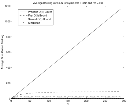
Figure 1: Simulation and Bounds for the ON/OFF system with symmetric traffic and $\rho=0.8$.

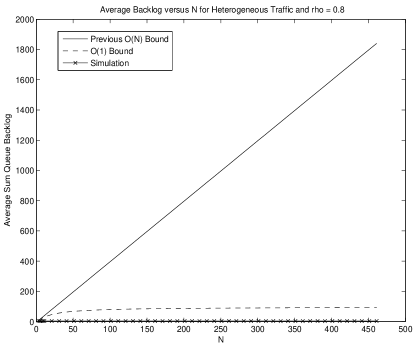
Figure 2: Simulation and Bounds for the ON/OFF system with heterogeneous traffic and $\rho=0.8$.

VII Conclusions

We have presented an improved delay analysis for the max-weight scheduling algorithm. For ON/OFF channels, max-weight is equivalent to Longest Connected Queue (LCQ), and yields average delay that is order-optimal, being independent of the network size $N$. If an $f$-balanced traffic assumption holds, average delay was shown to maintain independence of $N$ while allowing an improved asymptotic in $\rho$. For multi-rate channels, a delay bound of $O(N)$ applies. Conversely, it is shown for a simple multi-rate example that, unlike ON/OFF channels, average backlog must be at least linear in $N$ due to “residual” packets. Our delay analysis makes use of the technique of queue grouping. The particular Lyapunov functions introduced for this delay analysis are powerful and may be useful in other contexts.

Appendix A — Proof of Lemma 3

Here we prove Lemma 3. Define $\Delta_{1}({\boldsymbol{Q}}(t))$ and $\Delta_{2}({\boldsymbol{Q}}(t))$ as the conditional drift for the sum of squares term and the square of queue backlog term, respectively, so that $\Delta({\boldsymbol{Q}}(t))=\Delta_{1}({\boldsymbol{Q}}(t))+\theta\Delta_{2}({\boldsymbol{Q}}(t))$. Squaring (20) and using the fact that $\tilde{\mu}_{i}(t)^{2}=\tilde{\mu}_{i}(t)$ and $Q_{i}(t)\tilde{\mu}_{i}(t)=Q_{i}(t)\mu_{i}(t)$ (because $\tilde{\mu}_{i}(t)\in\{0,1\}$, and $\tilde{\mu}_{i}(t)=\mu_{i}(t)$ if $Q_{i}(t)>0$): yields:

$$\frac{1}{2}Q_{i}(t+1)^{2} = \frac{1}{2}Q_{i}(t)^{2}+\frac{(A_{i}(t)-\tilde{\mu}_{i}(t))^{2}}{2}$$

$$-Q_{i}(t)(\mu_{i}(t)-A_{i}(t))$$

$$= \frac{1}{2}\left[Q_{i}(t)^{2}+A_{i}(t)^{2}+\tilde{\mu}_{i}(t)\right]-A_{i}(t)\tilde{\mu}_{i}(t)$$

$$-Q_{i}(t)(\mu_{i}(t)-A_{i}(t))$$

Therefore:

$$\Delta_{1}({\boldsymbol{Q}}(t)) = \mathbb{E}\left\{B_{1}(t)\left|\right.{\boldsymbol{Q}}(t)\right\}$$

$$-\sum_{i=1}^{N}Q_{i}(t)\mathbb{E}\left\{\mu_{i}(t)-\lambda_{i}\left|\right.{\boldsymbol{Q}}(t)\right\}$$

where

$$B_{1}(t)\mbox{\raisebox{-1.29167pt}{$\overset{\vartriangle}{=}$}}\sum_{i=1}^{N}\left[\frac{1}{2}\left[A_{i}(t)^{2}+\tilde{\mu}_{i}(t)\right]-A_{i}(t)\tilde{\mu}_{i}(t)\right]$$

Similarly:

$$\frac{1}{2}Q_{tot}(t+1)^{2} = \frac{1}{2}\left[Q_{tot}(t)^{2}+\tilde{\mu}_{tot}(t)^{2}+A_{tot}(t)^{2}\right]$$

$$-\tilde{\mu}_{tot}(t)A_{tot}(t)$$

$$-Q_{tot}(t)(\tilde{\mu}_{tot}(t)-A_{tot}(t))$$

Therefore:

$$\Delta_{2}({\boldsymbol{Q}}(t)) = \mathbb{E}\left\{B_{2}(t)\left|\right.{\boldsymbol{Q}}(t)\right\}$$

$$-Q_{tot}(t)\mathbb{E}\left\{\tilde{\mu}_{tot}(t)-\lambda_{tot}\left|\right.{\boldsymbol{Q}}(t)\right\}$$

where $\tilde{\mu}_{tot}(t)^{2}=\tilde{\mu}_{tot}(t)$ (because it is either $0$ or $1$), and

$$B_{2}(t)\mbox{\raisebox{-1.29167pt}{$\overset{\vartriangle}{=}$}}\frac{1}{2}\left[\tilde{\mu}_{tot}(t)+A_{tot}(t)^{2}\right]-\tilde{\mu}_{tot}(t)A_{tot}(t)$$

Summing $\Delta_{1}({\boldsymbol{Q}}(t))$ and $\theta\Delta_{2}({\boldsymbol{Q}}(t))$ and noting from (23) that $B(t)=B_{1}(t)+\theta B_{2}(t)$ yields the result of Lemma 3.

Appendix B — Proof of Lemma 6

Define the integer $m=\hat{N}/K$. Here we prove Lemma 6. Given a particular queue backlog vector ${\boldsymbol{Q}}(t)$, the LCQ algorithm maximizes the expression $\sum_{i=1}^{\hat{N}}Q_{i}(t)\mu_{i}(t)$ over all ${\boldsymbol{\mu}}(t)\in{{{\cal{F}}}}(t)$. We now show that this also maximizes the expression given in Lemma 6. To this end, we have:

$$\sum_{g\in{{\cal{G}}}_{K}}\sum_{k=1}^{K}Q_{k}^{(g)}(t)\tilde{\mu}_{k}^{(g)}(t) = \sum_{g\in{{\cal{G}}}_{K}}\sum_{k=1}^{K}Q_{k}^{(g)}(t)\sum_{i\in{{\cal{L}}}_{k}^{(g)}}\tilde{\mu}_{i}(t)$$

$$=\sum_{i=1}^{\hat{N}}\tilde{\mu}_{i}(t)Q_{i}(t)\left|{{\cal{G}}}_{K}\right|$$

$$+\sum_{i=1}^{\hat{N}}\tilde{\mu}_{i}(t)\sum_{j\neq i}Q_{j}(t)\frac{\left|{{\cal{G}}}_{K}\right|(m-1)}{\hat{N}-1}$$

where the final equality holds because link $i$ is in every group that multiplies the $\tilde{\mu}_{i}(t)$ term, and all other links multiply this term the same number of times (by group symmetry). The above also uses the fact that (by symmetry) the number of group partitions for which a particular link $j$ is in the same group as link $i$ is equal to the total number of partitions multiplied by the probability that a randomly chosen partition includes $i$ and $j$ in the same group. Define the above expression as $f(t)$ for simplicity. Therefore:

$$f(t) = \sum_{i=1}^{\hat{N}}\tilde{\mu}_{i}(t)Q_{i}(t)\left|{{\cal{G}}}_{K}\right|(1-\frac{m-1}{\hat{N}-1})$$ (45)

$$+\sum_{i=1}^{\hat{N}}\tilde{\mu}_{i}(t)\left(\sum_{j=1}^{\hat{N}}Q_{j}(t)\right)\left|{{\cal{G}}}_{K}\right|\frac{m-1}{\hat{N}-1}$$

The $\tilde{\mu}_{i}(t)$ values in the expression for $f(t)$ are the only ones affected by the control action on slot $t$. The final term on the right hand side is given by $\sum_{i}\tilde{\mu}_{i}(t)$ (the total departures on slot $t$) multiplied by a non-negative constant. This final term is maximized by any work conserving policy that always transmits a packet when there is a non-empty connected queue. The first term on the right hand side is a non-negative constant multiplied by the term $\sum_{i}\tilde{\mu}_{i}(t)Q_{i}(t)$. But note that $\tilde{\mu}_{i}(t)Q_{i}(t)=\mu_{i}(t)Q_{i}(t)$, and thus the LCQ policy maximizes this first term. As LCQ is work conserving, it also maximizes the second term, and thus maximizes $f(t)$, proving Lemma 6.

Appendix C — Proof of Lemmas 7 and 8

Proof:

(Lemma 7) Define the integer $m=\hat{N}/K$. Using a counting argument similar to that of Appendix B (compare with (45)), we have that for any vector ${\boldsymbol{\lambda}}=(\lambda_{1},\ldots,\lambda_{\hat{N}})$:

$$\sum_{g\in{{\cal{G}}}_{K}}\sum_{k=1}^{K}Q_{k}^{(g)}(t)\lambda_{k}^{(g)} = \sum_{i=1}^{\hat{N}}Q_{i}(t)\lambda_{i}\left|{{\cal{G}}}_{K}\right|(1-\frac{m-1}{{\hat{N}}-1})$$ (46)

$$+Q_{tot}(t)\lambda_{tot}\left|{{\cal{G}}}_{K}\right|\frac{m-1}{{\hat{N}}-1}$$

Using the bound on $\lambda_{i}$ given in (37) yields:

$$\sum_{g\in{{\cal{G}}}_{K}}\sum_{k=1}^{K}Q_{k}^{(g)}(t)\lambda_{k}^{(g)}\leq\hskip 108.405pt$$

$$Q_{tot}(t)\lambda_{tot}\left|{{\cal{G}}}_{K}\right|\left[\frac{1}{{\hat{N}}}-\frac{m-1}{{\hat{N}}({\hat{N}}-1)}+\frac{m-1}{{\hat{N}}-1}\right]$$

$$+Q_{tot}(t)\left|{{\cal{G}}}_{K}\right|(1-\frac{m-1}{{\hat{N}}-1})\beta(1-\rho)/K$$

The result of Lemma 7 follows by using the identities:

$$\left[\frac{1}{{\hat{N}}}-\frac{m-1}{{\hat{N}}({\hat{N}}-1)}+\frac{m-1}{{\hat{N}}-1}\right]=\frac{1}{K}$$ (47)

$$\left[1-\frac{m-1}{\hat{N}-1}\right]=z$$

∎

Proof:

(Lemma 8) Let $L(t)$ represent the number of non-empty queues on slot $t$. If $L(t)=0$, then $Q_{tot}(t)=0$ and the result is trivial. Now suppose that $L(t)=l$, where $l\in\{1,2,\ldots,N\}$. Define $(l_{1},\ldots,l_{\hat{N}})$ to be a $0/1$ vector with $l_{i}=1$ if and only if $Q_{i}(t)>0$. Define $l_{k}^{(g)}$ to be the number of non-empty queues in the $k$th group of partition $g$. Consider the following randomized policy for ${\boldsymbol{\mu}}^{*}(t)\in{{{\cal{F}}}}(t)$: First observe all channel states $S_{i}(t)$ for non-empty queues $i$, and define new channel states $\hat{S}_{i}(t)$ as follows: If $S_{i}(t)=0$ (OFF), assign $\hat{S}_{i}(t)=0$. If $S_{i}(t)=1$ (ON), independently assign $\hat{S}_{i}(t)=1$ with probability $p_{min}/p_{i}$ (this is a valid probability because $p_{min}\leq p_{i}$). It follows that the new channel state vector $\hat{{\boldsymbol{S}}}(t)$ has independent and symmetric ON probabilities $p_{min}$. Now independently, randomly, and uniformly choose a queue to serve over all non-empty queues $i$ with $\hat{S}_{i}(t)=1$. It follows that for all non-empty queues $i$ we have:

$$\mathbb{E}\left\{\tilde{\mu}_{i}^{*}(t)\left|\right.{\boldsymbol{Q}}(t)\right\}=\frac{1-(1-p_{min})^{l}}{l}=\frac{r_{l}}{l}$$

Further, for any $g\in{{\cal{G}}}_{K}$ and any $k\in\{1,\ldots,K\}$ we have:

$$\mathbb{E}\left\{\tilde{\mu}_{k}^{(g)*}(t)\left|\right.{\boldsymbol{Q}}(t)\right\}=\sum_{i\in{{\cal{L}}}_{k}^{(g)}}\mathbb{E}\left\{\tilde{\mu}_{i}^{*}(t)\left|\right.{\boldsymbol{Q}}(t)\right\}=l_{k}^{(g)}\frac{r_{l}}{l}$$

Using this equality gives:

$$\sum_{g\in{{\cal{G}}}_{K}}\sum_{k=1}^{K}Q_{k}^{(g)}(t)\mathbb{E}\left\{\tilde{\mu}_{k}^{(g)*}(t)\left|\right.{\boldsymbol{Q}}(t)\right\}=$$

$$\frac{r_{l}}{l}\sum_{g\in{{\cal{G}}}_{K}}\sum_{k=1}^{K}Q_{k}^{(g)}(t)l_{k}^{(g)}$$ (48)

Now note that the $l_{k}^{(g)}$ values are structurally similar to the $\lambda_{k}^{(g)}$ values, and hence (similar to (46)) we have (using $Q_{i}(t)l_{i}=Q_{i}(t)$ and $l_{tot}=l$):

$$\sum_{g\in{{\cal{G}}}_{K}}\sum_{k=1}^{K}Q_{k}^{(g)}(t)l_{k}^{(g)} = \sum_{i=1}^{\hat{N}}Q_{i}(t)\left|{{\cal{G}}}_{K}\right|(1-\frac{m-1}{\hat{N}-1})$$

$$+Q_{tot}(t)l\left|{{\cal{G}}}_{K}\right|\frac{m-1}{\hat{N}-1}$$

Using this in (48) yields:

$$\sum_{g\in{{\cal{G}}}_{K}}\sum_{k=1}^{K}Q_{k}^{(g)}(t)\mathbb{E}\left\{\tilde{\mu}_{k}^{(g)*}(t)\left|\right.{\boldsymbol{Q}}(t)\right\}$$

$$=\frac{r_{l}}{l}Q_{tot}(t)\left|{{\cal{G}}}_{K}\right|\left[1-\frac{m-1}{\hat{N}-1}+\frac{l(m-1)}{\hat{N}-1}\right]$$ (49)

$$\geq r_{l}Q_{tot}(t)\left|{{\cal{G}}}_{K}\right|\left[\frac{1}{\hat{N}}-\frac{(m-1)}{\hat{N}(\hat{N}-1)}+\frac{m-1}{\hat{N}-1}\right]$$

$$=r_{l}Q_{tot}(t)\left|{{\cal{G}}}_{K}\right|/K$$ (50)

where the last equality holds by (47). The above holds for $L(t)=l\in\{1,\ldots,N\}$. Suppose now that $l\geq K$. In this case we have $r_{l}\geq r_{K}$, proving the result of Lemma 8 for $l\geq K$.

Consider now the final case where $l\in\{1,\ldots,K-1\}$. Then from (49) we have:

$$\sum_{g\in{{\cal{G}}}_{K}}\sum_{k=1}^{K}Q_{k}^{(g)}(t)\mathbb{E}\left\{\tilde{\mu}_{k}^{(g)*}(t)\left|\right.{\boldsymbol{Q}}(t)\right\}$$

$$\geq\frac{r_{l}}{l}Q_{tot}(t)\left|{{\cal{G}}}_{K}\right|$$ (51)

Using the fact that $\frac{r_{l}}{l}\geq\frac{r_{K-1}}{K-1}\geq\frac{r_{K}}{K}$ yields the result. ∎

Appendix D — Proof of Lemma 1

Here we prove that $\mu_{K}^{sym}>\mu_{K+1}^{sym}$. Specifically, we show that if $p$ is a value such that $0<p\leq 1$, then for any positive integer $K$ we have:

$$\frac{1}{K}[1-(1-p)^{K}]>\frac{1}{K+1}[1-(1-p)^{K+1}]$$ (52)

To show this, note that it is trivially true for the case $p=1$. In the opposite case where $0<p<1$, we can multiply (52) by $K(K+1)$ and rearrange terms to see that the inequality is equivalent to the following:

$$(1-p)^{K}+Kp(1-p)^{K}<1$$ (53)

Thus, it suffices to prove that (53) is true. To this end, we have:

$$(1-p)^{K}+Kp(1-p)^{K} < (1-p)^{K}+Kp(1-p)^{K-1}$$

$$\leq \sum_{i=0}^{K}{K\choose i}p^{i}(1-p)^{K-i}$$

$$= ((1-p)+p)^{K}=1$$

where the first (strict) inequality holds because $0<p<1$ and hence $(1-p)^{K}<(1-p)^{K-1}$. This establishes (53) and completes the proof of Lemma 1.

Appendix E — Proof of Lemma 10

The queueing dynamics are given by $Q_{i}(t+1)=Q_{i}(t)-\tilde{\mu}_{i}(t)+A_{i}(t)$, where $\tilde{\mu}_{i}(t)=\min[\mu_{i}(t),Q_{i}(t)]$. Using the Lyapunov function $L({\boldsymbol{Q}}(t))\mbox{\raisebox{-1.29167pt}{$\overset{\vartriangle}{=}$}}\frac{1}{2}\sum_{i=1}^{N}Q_{i}(t)^{2}$ and performing a standard quadratic drift computation (see, for example, [6]), it is not difficult to show the drift satisfies:

$$\Delta({\boldsymbol{Q}}(t)) = \frac{1}{2}\sum_{i=1}^{N}\mathbb{E}\left\{A_{i}(t)^{2}\right\}$$

$$-\sum_{i=1}^{N}\mathbb{E}\left\{\lambda_{i}\tilde{\mu}_{i}(t)-\frac{\tilde{\mu}_{i}(t)^{2}}{2}\left|\right.{\boldsymbol{Q}}(t)\right\}$$

$$+\sum_{i=1}^{N}\lambda_{i}Q_{i}(t)-\sum_{i=1}^{N}Q_{i}(t)\mathbb{E}\left\{\mu_{i}(t)\left|\right.{\boldsymbol{Q}}(t)\right\}$$

$$+\sum_{i=1}^{N}Q_{i}(t)\mathbb{E}\left\{\mu_{i}(t)-\tilde{\mu}_{i}(t)\left|\right.{\boldsymbol{Q}}(t)\right\}$$

By definition of $\tilde{\mu}_{i}(t)$, we have:

$$Q_{i}(t)(\mu_{i}(t)-\tilde{\mu}_{i}(t)) = \tilde{\mu}_{i}(t)\mu_{i}(t)-\tilde{\mu}_{i}(t)^{2}$$

$$\leq \min[\mu_{i,max}\tilde{\mu}_{i}(t),\mu_{i}(t)^{2}]-\tilde{\mu}_{i}(t)^{2}$$

Hence:

$$\Delta({\boldsymbol{Q}}(t)) \leq \frac{1}{2}\sum_{i=1}^{N}\mathbb{E}\left\{A_{i}(t)^{2}\right\}$$ (54)

$$-\sum_{i=1}^{N}\mathbb{E}\left\{\lambda_{i}\tilde{\mu}_{i}(t)+\frac{\tilde{\mu}_{i}(t)^{2}}{2}\left|\right.{\boldsymbol{Q}}(t)\right\}$$

$$+\sum_{i=1}^{N}\lambda_{i}Q_{i}(t)-\sum_{i=1}^{N}Q_{i}(t)\mathbb{E}\left\{\mu_{i}(t)\left|\right.{\boldsymbol{Q}}(t)\right\}$$

$$+\sum_{i=1}^{N}\mathbb{E}\left\{\min\left[\mu_{i,max}\tilde{\mu}_{i}(t),\mu_{i}(t)^{2}\right]\left|\right.{\boldsymbol{Q}}(t)\right\}$$

Using the fact that $\mathbb{E}\left\{\min[\cdot,\cdot]\right\}\leq\min[\mathbb{E}\left\{\cdot\right\},\mathbb{E}\left\{\cdot\right\}]$ (by Jensen’s inequality and concavity of the $\min[\cdot,\cdot]$ operator), that the sum of a $\min$ is less than or equal to the $\min$ of a sum, and that $\sum_{i=1}^{N}\mathbb{E}\left\{\mu_{i}(t)^{2}\left|\right.{\boldsymbol{Q}}(t)\right\}\leq\hat{S}^{2}$, the final term on the right hand side of (54) can be bounded by:

$$\min\left[\sum_{i=1}^{N}\mu_{i,max}\mathbb{E}\left\{\tilde{\mu}_{i}(t)\left|\right.{\boldsymbol{Q}}(t)\right\},\hat{S}^{2}\right]$$

Because the max-weight policy maximizes $\sum_{i=1}^{N}Q_{i}(t)\mu_{i}(t)$ (given queue backlogs ${\boldsymbol{Q}}(t)$) we have:

$$\sum_{i=1}^{N}Q_{i}(t)\mathbb{E}\left\{\mu_{i}(t)\left|\right.{\boldsymbol{Q}}(t)\right\}\geq\sum_{i=1}^{N}Q_{i}(t)\mathbb{E}\left\{\mu_{i}^{*}(t)\left|\right.{\boldsymbol{Q}}(t)\right\}$$ (55)

where $\mu_{i}^{*}(t)$ represents any alternative scheduling decision. Noting that ${\boldsymbol{\lambda}}/\rho\in\Lambda$ and ${\boldsymbol{\mu}}_{sym}/N\in\Lambda$, we have by convexity of $\Lambda$:

$${\boldsymbol{\lambda}}+(1-\rho){\boldsymbol{\mu}}_{sym}/N\in\Lambda$$

Thus, there exists a stationary randomized policy that chooses ${\boldsymbol{\mu}}^{*}(t)$ independent of queue backlog to yield:

$$\mathbb{E}\left\{{\boldsymbol{\mu}}^{*}(t)\left|\right.{\boldsymbol{Q}}(t)\right\}=\mathbb{E}\left\{{\boldsymbol{\mu}}^{*}(t)\right\}={\boldsymbol{\lambda}}+(1-\rho){\boldsymbol{\mu}}_{sym}/N$$

Plugging this into (55) and then into (54) yields:

$$\Delta({\boldsymbol{Q}}(t)) \leq \frac{1}{2}\sum_{i=1}^{N}\mathbb{E}\left\{A_{i}(t)^{2}\right\}$$ (56)

$$-\sum_{i=1}^{N}\mathbb{E}\left\{\lambda_{i}\tilde{\mu}_{i}(t)+\frac{\tilde{\mu}_{i}(t)^{2}}{2}\left|\right.{\boldsymbol{Q}}(t)\right\}$$

$$-\frac{(1-\rho)\mu_{sym}}{N}\sum_{i=1}^{N}Q_{i}(t)$$

$$+\min\left[\sum_{i=1}^{N}\mu_{i,max}\mathbb{E}\left\{\tilde{\mu}_{i}(t)\left|\right.{\boldsymbol{Q}}(t)\right\},\hat{S}^{2}\right]$$

Using the Lyapunov drift lemma (Lemma 4) on the above drift and noting that the system is stable with well defined time average limits yields:

$$\sum_{i=1}^{N}\overline{Q}_{i} \leq \frac{N\left[\frac{1}{2}\sum_{i=1}^{N}\mathbb{E}\left\{A_{i}^{2}\right\}-\frac{3}{2}\sum_{i=1}^{N}\lambda_{i}^{2}\right]}{(1-\rho)\mu_{sym}}$$

$$+\frac{N\min\left[\sum_{i=1}^{N}\lambda_{i}\mu_{i,max},\hat{S}^{2}\right]}{(1-\rho)\mu_{sym}}$$

where we have used the fact that $\lim_{t\rightarrow\infty}\mathbb{E}\left\{\tilde{\mu}_{i}(t)\right\}=\lambda_{i}$ and $\lim_{t\rightarrow\infty}\mathbb{E}\left\{\tilde{\mu}_{i}^{2}(t)\right\}\geq\lim_{t\rightarrow\infty}\mathbb{E}\left\{\tilde{\mu}_{i}(t)\right\}^{2}=\lambda_{i}^{2}$. Using Little’s theorem on this congestion bound proves (42).

Now suppose that all $S_{i}(t)$ processes are independent and $Pr[S_{i}(t)=\mu_{i,max}]\geq p_{min}$ for all $i$. We derive the bound on $\mu_{sym}$ given in Lemma 10. Define $\hat{\mu}\mbox{\raisebox{-1.29167pt}{$\overset{\vartriangle}{=}$}}\min_{i\in\{1,\ldots,N\}}\mu_{i,max}$. Consider the stationary and randomized algorithm ${\boldsymbol{\mu}}^{*}(t)$ that observes channel states ${\boldsymbol{S}}(t)$ and probabilistically places each link $i\in\{1,\ldots,N\}$ in a set $\chi(t)$ with probability $0$ if $S_{i}(t)<\hat{\mu}$, and with probability $p_{min}/Pr[S_{i}(t)\geq\hat{\mu}]$ if $S_{i}(t)\geq\hat{\mu}$. Then $\chi(t)$ contains a random number of links, and each link appears in $\chi(t)$ independently with probability $p_{min}$. Select a link to serve on slot $t$ uniformly and randomly with equal probability over all links in $\chi(t)$ (remaining idle if $\chi(t)$ is empty). It follows that under this policy, a particular link $i$ is selected for transmission with probability exactly $(1-(1-p_{min})^{N})/N$, and is selected only if $S_{i}(t)\geq\hat{\mu}$. Hence:

$$\mathbb{E}\left\{\mu_{i}^{*}(t)\right\}\geq\frac{\hat{\mu}(1-(1-p_{min})^{N})}{N}\>\>\mbox{ for all $i\in\{1,\ldots,N\}$}$$

It follows that the symmetric rate vector with all $N$ entries equal to the right hand side in the above expression is in the capacity region $\Lambda$, so that $\mu_{sym}/N$ is greater than or equal to this value.

References

- [1] M. J. Neely. Delay analysis for max weight opportunistic scheduling in wireless systems. Proc. 46th Annual Allerton Conf. on Communication, Control, and Computing, Sept. 2008.
- [2] L. Tassiulas and A. Ephremides. Dynamic server allocation to parallel queues with randomly varying connectivity. IEEE Transactions on Information Theory, vol. 39, pp. 466-478, March 1993.
- [3] N. Kahale and P. E. Wright. Dynamic global packet routing in wireless networks. Proc. IEEE INFOCOM, 1997.
- [4] M. Andrews, K. Kumaran, K. Ramanan, A. Stolyar, and P. Whiting. Providing quality of service over a shared wireless link. IEEE Communications Magazine, vol. 39, no.2, pp.150-154, 2001.
- [5] M. J. Neely, E. Modiano, and C. E. Rohrs. Power allocation and routing in multi-beam satellites with time varying channels. IEEE Transactions on Networking, vol. 11, no. 1, pp. 138-152, Feb. 2003.
- [6] L. Georgiadis, M. J. Neely, and L. Tassiulas. Resource allocation and cross-layer control in wireless networks. Foundations and Trends in Networking, vol. 1, no. 1, pp. 1-149, 2006.
- [7] M. J. Neely. Order optimal delay for opportunistic scheduling in multi-user wireless uplinks and downlinks. IEEE/ACM Transactions on Networking, vol. 16, no. 5, pp. 1188-1199, October 2008.
- [8] M. J. Neely, E. Modiano, and Y.-S. Cheng. Logarithmic delay for packet switches under the crossbar constraint. IEEE Transactions on Networking, vol. 15, no. 3, pp. 657-668, June 2007.
- [9] E. M. Yeh. Multiaccess and Fading in Communication Networks. PhD thesis, Massachusetts Institute of Technology, Laboratory for Information and Decision Systems (LIDS), 2001.
- [10] A. Ganti, E. Modiano, and J. N. Tsitsiklis. Optimal transmission scheduling in symmetric communication models with intermittent connectivity. IEEE Transactions on Information Theory, vol. 53, no. 3, March 2007.
- [11] S. Shakkottai, R. Srikant, and A. Stolyar. Pathwise optimality of the exponential scheduling rule for wireless channels. Advances in Applied Probability, vol. 36, no. 4, pp. 1021-1045, Dec. 2004.
- [12] V. J. Venkataramanan and X. Lin. Structural properties of ldp for queue-length based wireless scheduling algorithms. Proc. of 45th Annual Allerton Conference on Communication, Control, and Computing, Monticello, Illinois, September 2007.
- [13] A. Stolyar. Large deviations of queues under qos scheduling algorithms. Proc. of 44th Annual Allerton Conference on Communication, Control, and Computing, Monticello, Illinois, September 2006.
- [14] S. Deb, D. Shah, and S. Shakkottai. Fast matching algorithms for repetitive optimization: An application to switch scheduling. Proc. of 40th Annual Conference on Information Sciences and Systems (CISS), Princeton, NJ, March 2006.
- [15] M. J. Neely. Delay analysis for maximal scheduling in wireless networks with bursty traffic. Proc. IEEE INFOCOM, April 2008.
- [16] M. Alanyali and M. Dashouk. On power-of-choice in downlink transmission scheduling. Information Theory and Applications Workshop (ITA), University of California, San Diego, January 2008.
- [17] X. Wu, R. Srikant, and J. R. Perkins. Scheduling efficiency of distributed greedy scheduling algorithms in wireless networks. IEEE Transactions on Mobile Computing, June 2007.
- [18] M. J. Neely. Delay analysis for max weight opportunistic scheduling in wireless systems. arXiv:0806.2345v1, June 2008.