Synchronization and Information Transmission in Spatio-Temporal Networks of Deformable Units

Abstract

We study the relationship between synchronization and the rate with which information is exchanged between nodes in a spatio-temporal network that describes the dynamics of classical particles under a substrate Remoissenet-Peyrard potential. We also show how phase and complete synchronization can be detected in this network. The difficulty in detecting phase synchronization in such a network appears due to the highly non-coherent character of the particle dynamics which unables a proper definition of the phase dynamics. The difficulty in detecting complete synchronization appears due to the spatio character of the potential which results in an asymptotic state highly dependent on the initial state.

1. Introduction

The sine-Gordon potential and similar others have been used to model the dynamics of many systems in physics, biology and engineering [?,?,?,?,?,?,?,?]. However, in real physical systems, the shape of the substrate potential can deviate from the standard one with a direct incidence on the stability properties of the system. In physical situations, such as charge-density waves, Josephson junctions, or crystals with dislocations, the application of the standard sine-Gordon model becomes too restrictive. In recent years, a number of potentials whose shapes can be turned at wish have appeared in the literature of nonlinear dynamical systems  [?,?,?,?,?,?,?]. These more realistic potentials certainly provide richer insights onto the physics of reals systems than what is predicted using the conventional, rigid models such as the sine-Gordon, double-sine-Gordon and $\phi^{4}$ potentials. In particular, we can expect a more rich and complex synchronization phenomena in models of nonlinear oscillators involving them.

The purpose of the present paper is to study networks formed by oscillators under realistic shape deformable potentials. To model the network, we use the Remoisnet-Payrar potential, which has been extensively used in the literature to describe the disturbance of the sinusoidal shape of the substrate periodic potential of the Sine Gordon equation [?,?,?].

We are mainly interested in the complex relationship between synchronization and transmission of information. By synchronization, we mean complete synchronization (CS)  [?,?,?,?] and chaotic phase synchronization (PS)  [?]. The information point-of-view will be provided by the procedure described by Baptista et al. in Refs.  [?]. As we shall show synchronization and information are directly related in such an active network. The larger the synchronization is the larger the rate with which information is exchanged between nodes in the network, the so called mutual information rate (MIR).

Such relationship can be experimentally explored when one needs to observe how nodes are attached to each other in a real network. For situations where the nodes of the network are neither completely synchronous nor phase synchronous, the MIR provides one the level of connectivity. In addition, the MIR limits the amount of information that can be retrieved in some point of the network about an arbitrary external stimulus.

Due to the spatio character of the studied network, both approaches, the ones in Refs.  [?,?,?,?] and the ones in Refs.  [?] might face difficulties to be implemented and this work resolves many of them. In particular, we study networks which have node trajectories departing from randomly initial conditions. That creates a situation similar to the one observed in networks constructed with nodes presenting different parameters, when the methods in Ref.  [?] should be used with precaution.

Note that a quite number of physical objects allowing a model description with the aid of the sine-Gordon equation are known: arrays of forced damped pendula, vortices in long Josephson junctions, charge-density waves in quasi-one-dimensional conductors etc… [?,?]. For real physical systems, the account of various disturbances and of a more complex character of atomic interactions breaks the exact integrability of the initial sine-Gordon equation, leaving the possibility for describing the system dynamics in terms of the same quasi-particles which now interact with each other.

The rest of the paper is organized as follows: in Sec. 2. we explore the dynamics of the network in consideration and analyze the effect of the deformability parameter in the substrate potential on the stability synchronization of the network. In Sec. 3. we analyze phase synchronization in such networks, and Sec. 4. is devoted to the study of information transmission within the nodes of the network. Finally, we present the conclusions in Sec. 5..

2. Synchronization dynamics of the networks

2.1 Description of the networks

We first investigate the dynamical properties of a single particle in a deformable substrate potential. If we define the variable $x$ as the displacement of the particle in the potential well, then the equation of motion describing its dynamics reads

$$\ddot{x}+\lambda\dot{x}+\omega^{2}\displaystyle\frac{\partial V(x,r)}{\partial x}=\eta_{0}\cos\Psi t.$$ (1)

In this work we consider the following fixed set of parameters $\lambda=0.01,\omega=1,\eta_{0}=0.19$. The parameters $\Psi$ and $r$ will be varied.

Recall that $x$ is the coordinate variable which characterizes the behavior of the particle in the potential well $V(x,r)$. The new issues of our model under consideration are the following: we apply an AC force $\eta(t)=\eta_{0}\cos\Psi t$ to the particle and assume also the external viscous damping with a coefficient $\lambda$. In this work, $V(x,r)$ is a nonlinear potential with a deformable shape introduced by Remoissenet-Payrard to study the coherent structure in a network formed by a similar system. There are many versions of this potential, but we concentrate our analyses on the most general case defined as  [?,?,?,?,?,?,?]

$$V(x,r)=(1-r)^{2}\displaystyle\frac{1-\cos x}{1+r^{2}+2r\cos x}$$ (2)

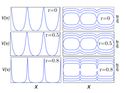
Figure  1.: Form of the potential as a function of $r$ and the corresponding periodic orbits for a free particle ($\eta_{0}$=0 and $\lambda=0$). The pictures in the left (right) column shows $x$ vs. $V(x,r)$ ($x$ vs. $\dot{x}$).

where the deformability parameter $r$ fulfills the condition $|r|<1$.

The advantageous feature of this potential can be summarized in the fact that it reproduces the sine Gordon ($r=0$) while avoiding most of it shortcomings. A shape of broad wells separated by narrow barriers can be obtained for $r>0$ and for $r<0$, a shape of deep narrow wells separated by broad gently sloping barriers can be obtained.

Figure 1 shows the form of the potential and the corresponding phase plane as a function of the parameter $r$, for $r>0$. One can observe that the larger the parameter $r$ is, the flatter the bottom of the potential.

In real physical systems, such potential can be produced by the interaction of an adatom with substrate atoms, where the parameter $r$ could account for the temperature or pressure dependence, or for the geometry of the surface of the metallic surface. It can be calculated from the first principles as described in Refs.  [?,?,?] (and reference therein). However it is more reliable to determine the parameter $r$ from experimental data. Estimates for e.g., a H/W adsystem (hydrogen atoms absorber on a tungsten surface), yield $r\approx-0.3$ [?,?,?]

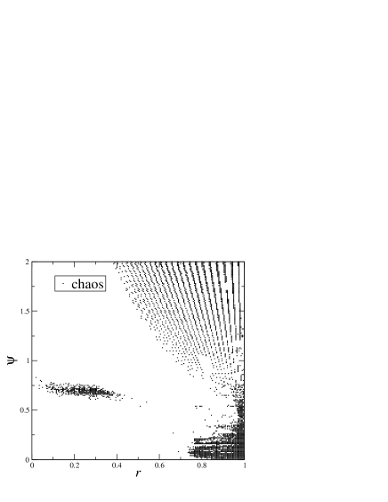
Figure  2.: Parameter space plot of the frequency $\psi$ and the deformability parameter $r$. Points represent chaotic behavior (positive KS-entropy and continuous Fourier spectrum).

Typically, if periodic oscillators are subjected to a periodic force, different phase-locking phenomena as well as chaos may be observed. And chaotic oscillators when subject to a periodic force give rise to a series of bifurcation phenomena.

Figure 2 shows the parameter space diagram of the oscillator in Eq. (1). Points (blank space) indicate values of the frequency $\Psi$ and the deformability parameter $r$ for which the oscillator in Eq. (1) is chaotic (periodic).

The $(r,\Psi)$ space is characterized by the predominance of periodic solutions. The chaotic solutions appear only for the value of the deformability parameter approaching the limit $1$. However for high frequency, the chaotic motion appears earlier, that is at $r\simeq 0.4$. For larger $r$ and $\Psi$ the parameter space presents a complex pattern whose chaotic regions appear side-by-side with periodic regions. For the specific narrow band of the frequency $\Psi$ around $0.70$ and $0.75$ a deep band of chaotic motion can be found for $r$ between $0.1$ and $0.4$. This confirms the chaotic behavior of deformable models systems as first suggested in references  [?,?,?].

We now consider a network of $N$ dynamical units of oscillators described by equations (1) and (2). The governing equation for the network is given by:

$$\dot{p_{i}} = n_{i}$$ (3)

$$\dot{n_{i}} = -\lambda n_{i}-\omega^{2}\displaystyle\frac{\partial V(p_{i},r)}{\partial p_{i}}+\eta_{0}\cos\Psi t$$ (5)

$$+g_{l}(p_{i+1}-2p_{i}+p_{i-1})\>\>\>\>\>\>\>\textrm{with}\>\>\>\>\>\>i=1,2...,N$$

where $V(p_{i},r)$ is given by Eq. (2). The constant parameter $g_{l}$ determines the strength of the coupling and $N$ the number of oscillators coupled. This equation is known as the Frenkel-Kontorova(FK) model with harmonic interaction and non-sinusoidal substrate potential. It has been extensively studied in the research of static characteristics of kinks (topological solitons) such as the effective mass, shape, and amplitude of the Peierls potential, the interaction energy of kinks, and the creation energy of kink-antikink pairs. The applicability of the extended Frenkel-Kontorova model for describing diffusion characteristics of a quasi-one-dimensional layer adsorbed on a crystal surface has also been discussed in Ref.  [?]. For real physical systems, the account of various disturbances and of a more complex character of atomic interactions break the exact integrability of the initial Sine Gordon equation, leaving the possibility for describing the system dynamics in terms of the same quasi-particles which interact with each other. This interaction, which is due to the departure from complete integrability, results in the following effects. The kolmogorov-Sinai entropy becomes nonzero and the Fourier spectrum of excited states of the system becomes continuous. Both characteristics of chaos.

2.2 Stability of the synchronization

Our analysis will be limited to networks of identical units. Since the $N$ systems are identical, it exists an exactly synchronized solution of Eq. (3), and the synchronization manifold is defined by $\mathcal{M}$=$\{p_{1}=p_{2}=....=p_{N}=p_{s};n_{1}=n_{2}=....=n_{N}=n_{s}\}$.

In the study of synchronization, a very relevant problem is to assess the conditions for the stability of the synchronous behavior for the networks and for the coupling configuration. The master stability function approach was originally introduced for arrays of coupled oscillators  [?], and it has been latter extended to the case of complex networks of dynamical systems  [?,?]. To use this, let us consider $N$ coupled dynamical units, each of them giving rise to the evolution of 2-dimensional vector fields $x_{i}$ ruled by a local set of ordinary differential equations $\dot{x}_{i}=\textbf{F}(x_{i})$. The equations of motion using the new variable can be written as

$$\dot{x}_{i}=\textbf{F}(x_{i})+g_{l}\sum_{j=1}^{N}G_{ij}\textbf{H}(x_{j}),\qquad i=1,2,...,N,$$ (6)

where $\dot{x}_{i}=\textbf{F}(x_{i})$ governs the local dynamics of the $i$th node. $x_{i}=[p_{i},n_{i}]^{T},$ and $\textbf{F}(x_{i})=\left[n_{i},-\lambda n_{i}-\omega^{2}\frac{\partial V(p_{i},r)}{\partial p_{i}}+\eta_{0}\cos\Psi t\right]^{T}$ with $V(p_{i},r)$ as in Eq.(2), the output function $\textbf{H}(x_{i})$ is a vectorial function defined trough the matrix $\mathbf{E}$=$\left(\begin{array}[]{cc}0&0\\ 1&0\end{array}\right)$ by $\textbf{H}(x_{i})=$ $\mathbf{E}$ $x_{i}$ , and $G(t)$ is a symmetric Laplacian matrix ($\sum_{j}G_{ij}=0$) describing the networks connection and given by

$$\mathbf{G}=\left(\begin{array}[]{ccccc}-2&1&0&\ldots&1\\ 1&-2&1&\ldots&0\\ 0&1&-2&\ldots&0\\ \vdots&\vdots&\vdots&\ddots&1\\ 1&0&\ldots&1&-2\end{array}\right)$$

The stability of the synchronization state can be determined from the variational equations obtained by considering an infinitesimal perturbation $\delta x_{i}$ from the synchronous states, $p_{i}=\delta p_{i}+p_{s}$, $n_{i}=\delta n_{i}+n_{s}$. The equations of motion for the perturbation $\delta x_{i}$ can be straightforwardly obtained by expanding the Eq. (6) in Taylor series of first order around the synchronized state which gives

$$\delta{\dot{x}}_{i} = D\textbf{F}(x_{s})\delta x_{i}+g_{l}\sum_{j=1}^{N}G_{ij}D\textbf{H}(x_{s})\delta x_{i},\>\>\>\>\>\>\>\>i=1,2,...,N,$$ (7)

$$= \sum_{j=1}^{N}\left[D\textbf{F}(x_{s})\delta_{ij}+g_{l}G_{ij}D\textbf{H}(x_{s})\right]\cdot\delta x_{i},\>\>\>\>\>\>i=1,2,...,N,$$ (8)

where $D\textbf{F}$ and $D\textbf{H}$ are the Jacobians of the vector field and the output function respectively.

Equation (5) is referred to as the variational equation and is often the starting point for stability determination. This equation is rather complicated since given arbitrary coupling $G$ it can be quite high dimensional. However, we can simplify the problem by noticing that the arbitrary state $\delta x_{i}$ can be written as $\delta x_{i}=\sum_{i=1}^{N}\textbf{v}_{i}\bigotimes\xi_{i}(t)$ with $\xi_{i}(t)=(\xi_{1,i},\xi_{2,i})$ where $\gamma_{i}$ and $\textbf{v}_{i}$ are the set of real eigenvalues and the associated orthogonal eigenvector of the matrix $G$ respectively, such that $G\textbf{v}_{i}=\gamma_{i}\textbf{v}_{i}$ and $\textbf{v}_{i}^{T}\textbf{v}_{i}=\delta_{ij}$. By applying $\textbf{v}_{i}^{T}(t)$ (and $v_{i}$) to the left (right) side of each term in Eq. (7) one finally obtains a set of N blocks for the coefficients $\xi_{i}(t)$. The first term with the Kronecker delta remains the same. This results in a variational equation in the eigenmode form

$$\dot{\xi}_{k}=\left[D\textbf{F}(x_{s})+g_{l}\gamma_{k}D\textbf{H}(x_{s})\right]\xi_{k},k=0,1,2,...,N-1,$$ (9)

We recall that $\gamma_{k}$ are the eigenvalues of $G$, and are given by $\gamma_{k}=-4\sin^{2}(\pi k/N)$ for the diffusive coupling  [?]. Note that each equation in Eq. (9) corresponds to a set of 2 conditional Lyapunov exponents $\lambda_{k}^{j}$ (j=1,2) along the eigenmode corresponding to the specific eigenvalue $\gamma_{k}$. For $k=0$, we have the variational equation for the synchronization manifold $(\gamma_{0}=0)$ and its maximum conditional Lyapunov exponent $\lambda^{1}_{0}$ corresponds to the one of the isolated dynamical unit. The remaining variations $\xi_{k}$, k=1,2,…,N-1 are transverse to $\mathcal{M}$, and describe the system’s response to small deviations from the synchronization manifold. Any deviation from the synchronization manifold will be reflected in the growth of one or more of these variations. The stability of the synchronized state is ensured if arbitrary small transverse variations decay to zero. So, CS exists if $\lambda^{1}_{k}<0$, for $k\geq 1$.

We also calculate the condition for the synchronization in the network by using the Lyapunov spectra, calculated directly from Eq. (7). Complete synchronization in the generalized sense as defined in Refs.  [?,?] exists if the second largest Lyapunov exponent is negative.

Due to the periodic potential in Eq. (2), the active network in Eq. (6) is highly sensitive to initial conditions. As a consequence, networks whose elements have random initial conditions that differ only slightly completely synchronize for a coupling strength smaller than the coupling strength needed to completely synchronize networks that have elements whose initial conditions differ moderately. Often, the network never complete synchronizes, and one can only have that $|x_{k}-x_{l}|<\vartheta$, and so, the trajectory is never perfectly along the synchronization manifold. Even thought $\vartheta$ might be small, it is sufficiently large in order to mislead the statement that complete synchronization appears by only checking the conditional exponents. This discrepancy is due to the fact that, in this system, when the initial conditions are not too close, the systems goes to different attractors and the approximation made to obtain the conditional lyapunov exponents [Eq. (9)] is no longer completely valid, thought it provides still approximate results. The effect of having nodes with different initial conditions in the studied network is similar to having networks with different parameters.

In Fig. 3, we show the parameter spaces (coupling $g_{l}$ vs. deformability parameter $r$) of the complete synchronization regime. Points show the values of $g_{l}$ and $r$ for which all the transversal ($k\geq 1$) conditional exponents are negative [Figs. 3(A),(C)] or when the second largest Lyapunov exponent becomes negative [Figs. 3(B),(D)].

When the initial conditions differ by no more than 0.01 [Figs. 3(A-B)] the two conditions to predict complete synchronization provide the same surface in the parameter space. However, when these initial conditions differ by no more than 0.5 [Figs. 3(C-D)], the conditional exponents predict the appearance of complete synchronization for a coupling strength smaller than the strength for which it really appears, as predicted by the value of the second largest Lyapunov exponents [Figs. 3(D)].

One can also observe from these figures that as the deformability parameter increases, the system becomes more and more unstable. When $r>9.5$, it is almost not possible to find complete synchronization in the network for low values of coupling strength $g_{l}$. So, when the potential $V(P_{i},r)$ has a flat bottom, the particles are almost non-synchronizable in the network.

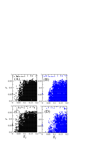
Figure  3.: Appearance of complete synchronization in a network of $N$=5 diffusively coupled oscillators. Points represent $g_{l}$ and $r$ values for which the conditional exponent $\lambda^{1}_{1}$ is negative (A,C) and for which the second largest Lyapunov exponent is negative (B,D). In (A,B), the initial conditions differ by at most 0.01 and in (C,D) the initial conditions differ by at most 0.5.

3. Phase synchronization

Phase synchronization  [?,?,?] is a phenomenon defined by

$$|\phi_{k}-m\phi_{l}|\leq\epsilon,$$ (10)

where $\phi_{k}$ and $\phi_{l}$ are the phases of the nodes $x_{k}$ and $x_{l}$ in the network [Eqs.(3)] and $m=\omega_{l}/\omega_{k}$, where $\omega_{k}$ and $\omega_{l}$ are the average frequencies of oscillation of these nodes, and $\epsilon$ is a finite number. In this work, we have used in Eq. (10) $m=1$, which means that we search for $\omega_{k}:\omega_{l}$=1:1 (rational) phase synchronization. If another type of $\omega_{k}:\omega_{l}$-PS is present, the methods in Refs.  [?] can detect.

The phase $\phi$ is a function constructed on a good 2D subspace, whose trajectory projection has proper rotation, i.e, it rotates around a well defined center of rotation. Often, a good 2D subspace is formed by the velocity space. In the oscillator considered in this work, one can use the results of  [?], and define the phase of the oscillator $x_{i}$ in Eqs. (3) as

$$\phi(t)=\int_{0}^{t}\frac{\ddot{n}_{i}\dot{p}_{i}-\ddot{p}_{i}\dot{n}_{i}}{{(\dot{p}_{i}^{2}+\dot{n}_{i}^{2})}}dt.$$ (11)

However, the oscillators in Eqs. (3) for the considered parameters have not a well defined phase, and even in a state where complete synchronization is achieved, one cannot use Eq. (11) to verify whether PS exists.

In short, if PS exists, in a subspace, then the points obtained from observations of the position of one node’s trajectory at the time another node makes any physical event do not visit the neighborhood of a special curve $\Gamma$, in this subspace. A curve $\Gamma$ is defined in the following way. Given a point $x_{0}$ in the attractor projected onto the subspace of one oscillator where the phase is defined, $\Gamma$ is the union of all points for which the phase, calculated from this initial point $x_{0}$ reaches $n\langle r\rangle$, with $n=1,2,3,\ldots,\infty$ and $\langle r\rangle$ a constant, usually 2$\pi$. Clearly an infinite number of curves $\Gamma$ can be defined.

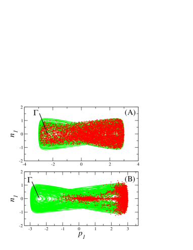
Figure  4.: The appearance of phase synchronization in two bidirectionally coupled oscillators. (A) There is no phase synchronization and the conditional observations are not localized with respect to the curve $\Gamma$ pictorially represented in the figure. (B) There is evidence of phase synchronization and the conditional observations are localized. Simulations are done considering initial conditions no more than 0.01 apart.

Formally, for non-coherent dynamical systems for which phase is still not well defined, PS implies localization of the conditional sets  [?], but the contrary is not always true. Therefore, finding localized sets should be considered a strong evidence that PS exists.

As an example, consider Eqs. (3) with two coupled oscillators, $r$=0.9, and $\phi=0.08$. For a small coupling $g_{l}$=0.01, in Fig. 4(A), we show a situation that PS is not present for $g_{l}$=0.01 and in Fig. 4(B), an evidence that PS exists, for $g_{l}$=0.05. The curve $\Gamma$, a continuous curve transversal to the trajectory, is pictorially represented by the straight line $\Gamma$. In 4(A), the conditional observations are not localized and thus there is no PS in this subspace. The light gray line (green online) represents the attractor projection on the subspace $(p_{i},n_{i})$ of the oscillator $x_{1}$, and filled gray circles (red online) represent the points obtained from the conditional observations of the oscillator $x_{1}$ whenever the oscillator $x_{2}$ makes an event. An event is considered to be the crossing of the trajectory to the line $n_{2}=0$, for $p_{2}>0$.

To have a general picture of when PS might appear in the two coupled oscillators, we show in Fig. 5(A) the quantity $\kappa$ with respect to $g_{l}$, defined as

$$\kappa=\frac{\max{(p_{1}^{i})-\min{(p_{1}^{i})}}}{\max{(p_{1}(t))-\min{(p_{1}(t))}}}$$ (12)

where $p_{1}^{i}$ represents the value of $p_{1}$ at the instant the trajectory of oscillator $x_{2}$ makes an event. Therefore, $\kappa$ is related to how broad the conditional observations visit the attractor. In Fig. 5(B) we show a few values of $p_{1}^{i}$ with respect to $g_{l}$. For $g_{l}\geq 0.06$, CS takes place.

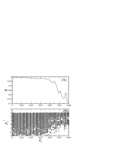
Figure  5.: The appearance of phase synchronization in two bidirectionally coupled oscillators. (A) Occupation of the conditional observations with respect to the attractor, $\kappa$, and in (B) the position variable $p_{1}^{i}$ when the oscillator $x_{2}$ makes the $i$th crossing with the section $n_{2}$=0, for $p_{2}>0$.

For large networks composed of $N$ nodes, this analysis is straightforward and PS between two nodes can be stated if the conditional observations realized in one node, whenever the other node makes an event, produces a localized set.

4. Information Transmission in the Network

In order to study the way information is transmitted in active networks, we introduce quantities and terminologies that assist us to better present our ideas and approaches.

The mutual information rate (MIR) is the rate with which information is being exchanged between two oscillation modes or elements in the active network.

The channel capacity, $\mathcal{C}_{C}$, is defined as the maximal possible amount of information that two oscillation modes or nodes within the network with a given topology can exchange, a local measure that quantifies the point-to-point rate with which information is being transmitted.

The Kolmogorov-Sinai entropy offers an appropriate way of obtaining the entropy production of a dynamical system. In chaotic systems, the entropy equals the summation of all the positive Lyapunov exponents ( [?]). Here, it provides a global measure of how much information can be simultaneously transmitted among all pairs of oscillation modes or nodes. Therefore, the KS-entropy, $H_{KS}$, of an active network, calculated for a given coupling strength, bounds the MIR between two oscillation modes, $I$, calculated for the same coupling strength. Thus,

$$I\leq H_{KS}$$ (13)

An active network is said to be self-excitable (non-self-excitable) when $\mathcal{C}_{C}$ $>H_{KS}^{(0)}$ (when $\mathcal{C}_{C}$ $\leq H_{KS}^{(0)}$), with $H_{KS}^{(0)}$ representing the KS entropy of one of the $N$ elements forming the active network, before they are coupled.

According to  [?], the upper bound for the MIR between two oscillation modes in an non-self-excitable active network, denoted as $I$, can be calculated by

$$I^{k}\leq\lambda_{0}^{1}-\lambda_{k}^{1}$$ (14)

where $\lambda_{0}^{1}$ and $\lambda_{k}^{1}$ ($k=1,\ldots,N-1$) are the positive largest conditional exponent  [?], numerically obtained from Eq. (9), with the oscillators possessing equal initial conditions. $\lambda_{0}$ measures the exponential divergence of trajectories along the synchronization manifold and $\lambda_{k}$ along the transversal modes. The units used for the MIR is [bits/unit time], which can be obtained by dividing Eq. (14) by $\log_{e}(2)$.

The networks as in Eq. (6) are predominantly of the non-self-excitable type. Only for a very small coupling strength, and a larger number of nodes, the network has a negligible increase of the KS-entropy, which we will disregard.

As can be seen from the $H_{KS}$ curve in Fig. 6, the two coupled oscillators are of the non-self-excitable type, since $H_{KS}^{(0)}=H_{KS}(g_{l}=0)/2$ which is approximately equal to $\mathcal{C}_{C}$. In this figure, we also show the MIR exchanged between the two coupled oscillators. As typically happens for non-excitable networks, the channel capacity is reached when the network complete synchronizes. Since the network is composed of two bidirectionally coupled systems, the MIR between the only two existing modes is actually the MIR between the two oscillators.

Comparing Figs. 5(A) and 6, one can see that there is a direct relationship between synchronization and information. The larger the amount of synchronization the larger the MIR, again another typical character of non-excitable networks.

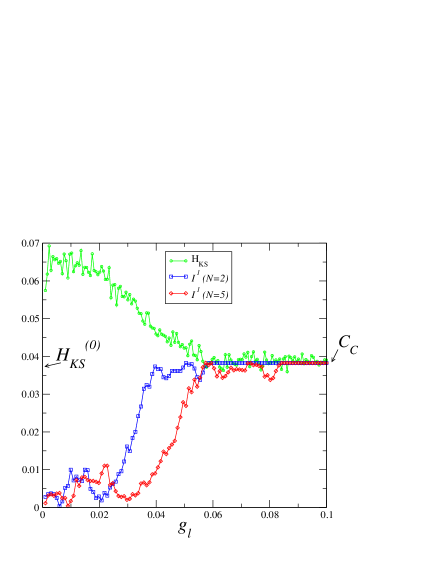
Figure  6.: [Color online] (green) Circles show the KS-entropy $H_{KS}$ and (blue) squares the MIR, $I^{1}$, for two bidirectional coupled oscillators. (red) Diamonds show $I^{1}$ for a network of $N$=5 diffusively coupled oscillators.

For larger networks with arbitrary topologies, the MIR between oscillation modes is just a rescaled version of the MIR between two coupled oscillators. Given that $g^{(2)}_{l}$ is the coupling strength for which complete synchronization takes place in two coupled oscillators, and therefore this coupled system operates with its channel capacity, the coupling strength for which complete synchronization takes place in a whole network composed of $N$ nodes with a certain topology is given by $g^{(N)}_{l}$

$$g^{(N)}_{l}=2\displaystyle\frac{g^{(2)}_{l}}{\gamma^{1}_{1}(N)}\>\>\>\>\>$$ (15)

At the parameter $g^{(N)}_{l}$, every pair of oscillators operate with the channel capacity. Equation (15) means that having the curve for the MIR for two coupled oscillators, the curve of the MIR for larger networks is rescaled by the second largest conditional Lyapunov exponent of the Laplacian matrix $\gamma^{1}_{1}(N)$.

As an illustration of Eq. (15), we show in Fig. 6, the MIR for a network composed of 5 oscillators coupled diffusively. In this figure, we show the quantity $\langle I\rangle$ defined as $\langle I\rangle=1/(N-1)\sum_{1}^{N-1}I^{k}$. Note that even though $\langle I\rangle$ might change its values according to the network topology and $N$, its maximal value is bounded by the channel capacity, which do not depends on the $N$ and the topology, another typical characteristic of non-self-excitable networks.

5. Conclusion

We study the relationship between synchronization and the rate with which information is exchanged between nodes in a spatio-temporal network which describes the dynamics of classical particles under a substrate Remoissenet-Peyrard potential. In particular, we study networks formed by Frenkel-Kontorova(FK) oscillators suffering the action of harmonic interaction and non-sinusoidal substrate potential.

We show that such networks are predominantly of the non-self-excitable type, i.e. as the coupling strength among the nodes increases the KS-entropy decreases. Other additional characteristics of non-self-excitable networks are: the mutual information rate (MIR) and the synchronization level increase simultaneously as the KS-entropy decreases; the channel capacity, the maximal of the MIR, is achieved for the same coupling strength for which complete synchronization appears.

We have overcome two difficulties concerning the detection of phase and complete synchronization in this complex spatio-temporal network. Even though the phase dynamics of each oscillator is not well defined, we have implement a technique which allows to evidence the presence of phase synchronization, by detecting the presence of localized sets obtained by the conditional observations. The more localized the sets are (which implies larger amount of phase synchrony) the larger the MIR. Concerning complete synchronization, we show that the master stability equation which provides the stability of the normal transversal modes (providing conditions to state complete synchronization) should be used with caution in such a network. The reason is that the final state is highly dependent on the initial conditions, a consequence of the spatio character provided by the potential. For that reason, in case the nodes have sufficiently different initial conditions, one should only state complete synchronization using the master stability equation in an approximate sense. A more rigorous condition to state complete synchronization is provided by the verification that the second largest Lyapunov exponent is negative.

Finally, we have shown how one can calculate the MIR between oscillation modes in larger networks with different topologies using as the only input information the curve of the MIR with respect to the coupling strength for two bidirectionally coupled oscillators. Having the curve for the MIR for two coupled oscillators, the curve of the MIR for larger networks is rescaled by the second largest conditional Lyapunov exponent of the Laplacian matrix of the larger network, the matrix that describes the way the nodes are connected in the network. That enables one to construct larger networks based on the dynamical characteristics of only two coupled oscillators.

REFERENCES

- [1] O. M. Braun and Y. S. Kivshar, Phys. Rep. 306, 1 (1998); O. M. Braun , Bambi Hu, and A. Zeltser, Phys Rev E 41, 4235 (2000); O. M. Braun , Y. S. Kivshar, and I. I. Zelenskaya, Phys Rev B 41, 7118 (1990).
- [2] M. Remoissenet, Waves called solitons: Concepts and experiments, (Springer Verlag 1999).
- [3] M. Peyrard and M. Remoissenet, Phys Rev B 26, 2886 (1982); M. Remoissenet and M. Peyrard, Phys Rev B 29, 3153 (1984).
- [4] G. Djuidje Kenmoe, A. Kenfack Jiotsa, and T. C. Kofane, Physica D 191 , 31 (2004).
- [5] T. C. Kofané, J Phys: Condens Matter 11, 2481 (1999).
- [6] J. P. Nguenang , J. A. Kenfack, and T. C. Kofané, Journal of Physics: Condensed Matter 16, 373 (2004).
- [7] L. Nana , T. C. Kofané , E. Coquet, and P. Tchofo-Dinda, Chaos, Solitons & Fractals 12, 73 (2001).
- [8] S. B. Yamgoué , T. C. Kofané, Chaos, Solitons & Fractals 15, 119 (2003); Chaos, Solitons & Fractals 15, 155 (2003).
- [9] S. Boccaletti, V. Latora, Y. Moreno, M. Chavez, and D.-H. Hwang, Phys. Rep. 424, 175 (2000).
- [10] L. M. Pecora and T. L. Carrol, Phys. Rev. Lett. 64, 821 (1990); L. M. Pecora and T. L. Carroll, Phys. Rev. Lett. 80, 2109 (1998).
- [11] R. Yamapi and S. Boccaletti, Phys. Lett A 371, 48 (2007).
- [12] M. Chavez, D.-H. Hwang , and S. Boccaletti, Eur. Phys. J.: Special Topics 146, 129 (2007).
- [13] A. Pikovsky, M. Rosenblum, and J. Kurths. Synchronization: A universal concept in nonlinear sciences (Cambridge University Press, London 2003).
- [14] M. S. Baptista and J. Kurths, Phys. Rev. E 72, 045202R (2005); M. S. Baptista and J. Kurths, Phys. Rev. E, 77, 026205 (2008); M. S. Baptista, S. P. Garcia, S. K. Dana, and J. Kurths, Transmission of information and synchronization in active networks: an experimental overview (to appear in Europhysics Journal); M. S. Baptista et al., Optimal network topology for information transmission in active networks arXiv:0804.2983v1.
- [15] M. S. Baptista, T. Pereira, J. C. Sartorelli, et al., Physica D 212, 216 (2005).
- [16] T. Pereira, M. S. Baptista, and J. Kurths, Phys. Rev. E, 75, 026216 (2007); T. Pereira, M. S. Baptista, and J. Kurths, Phys. Lett. A, 362, 159 (2007).
- [17] Ya. B. Pesin, Russian Math. Surveys 32, 55 (1977).