Abstract

Critical properties of the compact three-dimensional $U(1)$ lattice gauge theory are explored at finite temperatures on an asymmetric lattice. For vanishing value of the spatial gauge coupling one obtains an effective two-dimensional spin model which describes the interaction between Polyakov loops. We study numerically the effective spin model for $N_{t}=1,4,8$ on lattices with spatial extension ranging from $L=64$ to $L=256$. Our results indicate that the finite-temperature $U(1)$ lattice gauge theory belongs to the universality class of the two-dimensional $XY$ model, thus supporting the Svetitsky-Yaffe conjecture.

  e-mail addresses: ^∗oleg@bitp.kiev.ua, ^∗∗gravina,papa@cs.infn.it

1 Introduction

The finite temperature behavior of the compact three-dimensional ($3d$) $U(1)$ lattice gauge theory (LGT) is the subject of numerous investigations (see, e.g., Ref. [1] and references therein). It is well-known that at zero temperature the theory is confining at all values of the bare coupling constant [2]. At finite temperature the theory undergoes a deconfinement phase transition. Both phenomena are expected to take place in $4d$ QCD as well. Therefore, the $3d$ $U(1)$ gauge theory constitutes one of the simplest models with continuous gauge symmetry which possess the same fundamental properties as QCD. In view of these common features the critical properties of $3d$ $U(1)$ LGT deserve comprehensive qualitative and quantitative understanding.

On the theoretical side one should mention two results regarding the critical behavior of $3d$ $U(1)$ LGT. The first result states that the partition function of $3d$ $U(1)$ LGT in the Villain formulation coincides with that of the $2d$ $XY$ model in the leading order of the high-temperature expansion [3]. In particular, the monopoles of the original $U(1)$ gauge theory are reduced to vortices of the $2d$ system. The second result follows from the Svetitsky-Yaffe conjecture: the finite-temperature phase transition in the $3d$ $U(1)$ LGT should belong to the universality class of the $2d$ $XY$ model if correlation length diverges [4]. Then, two possibilities arise: either the transition is first order or it is the same transition which occurs in the $2d$ $XY$ model. The $XY$ model is known to have Berezinskii-Kosterlitz-Thouless (BKT) phase transition of infinite order [5, 6]. Several important facts could be deduced from these results. First of all, the global $U(1)$ symmetry cannot be broken spontaneously even at high temperatures because of the Mermin-Wagner theorem. Consequently, a local order parameter does not exist. Secondly, one might expect the critical behavior of the Polyakov loop correlation function $\Gamma(R)$ to be governed by the following expressions

$$\Gamma(R)\ \asymp\ \frac{1}{R^{\eta(T)}}\ ,$$ (1)

for $\beta\geq\beta_{c}$ and

$$\Gamma(R)\ \asymp\ \exp\left[-R/\xi(t)\right]\ ,$$ (2)

for $\beta<\beta_{c}$, $t=\beta_{c}/\beta-1$. Here, $R\gg 1$ is the distance between test charges and $\xi\sim e^{bt^{-\nu}}$ is the correlation length. Such behavior of $\xi$ defines the so-called essential scaling. The critical indices $\eta(T)$ and $\nu$ are known from the renormalization-group analysis of the $XY$ model: $\eta(T_{c})=1/4$ and $\nu=1/2$, where $T_{c}$ is the BKT critical point. Therefore, the critical indices $\eta$ and $\nu$ should be the same in the finite-temperature $U(1)$ model if the Svetitsky-Yaffe conjecture holds in this case.

The first renormalization-group calculations of the critical indices, presented in [4], gave support to the conjecture even though they did not constitute a rigorous proof. The direct numerical check of these predictions was performed on lattices $N_{s}^{2}\times N_{t}$ with $N_{s}=16,32$ and $N_{t}=4,6,8$ in Ref. [7]. Though authors of Ref. [7] confirm the expected BKT nature of the phase transition, the reported critical index is almost three times that predicted for the $XY$ model, $\eta(T_{c})\approx 0.78$. More recent numerical simulations of Ref. [1] have been mostly concentrated on the study of the properties of the high-temperature phase. We have to conclude that, so far, there are no numerical indications that the critical indices of $3d$ $U(1)$ LGT do coincide with those of the $2d$ $XY$ model. Moreover, since a rigorous determination of the critical indices is not available even for the $XY$ model one can hardly hope for a rigorous analysis of the critical behavior of $3d$ $U(1)$ LGT.

The absence of reliable results in the vicinity of the BKT critical point was our primary motivation to study the deconfinement phase transition in $3d$ $U(1)$ LGT. The difficulties in computations of critical indices of the $XY$ model are well-known and we do not intend to discuss them here (see Ref. [8] for a summary of recent results and problems). It should be clear however, that in the context of the $3d$ theory a reliable determination of critical properties becomes even harder and requires simulations on very large lattices. We have decided therefore to attack the problem in a few steps. Consider the finite-temperature model on anisotropic lattice with different spatial and temporal coupling constants; as a first step, in this paper we investigate the limit of vanishing spatial coupling. The major advantage of this limit is that the integration over spatial links can be performed analytically. The result of such integration is an effective two-dimensional spin model for the Polyakov loops. The latter can be studied numerically.

This paper is organized as follows. In the next section we introduce the compact $U(1)$ LGT on anisotropic lattice and study it for vanishing spatial coupling. In the Section 3 we describe briefly our numerical procedure. The result of simulations are presented in the Section 4. Conclusions and perspectives are given in the Section 5.

2 The 3$d$ U(1) lattice gauge theory

We work on a $3d$ lattice $\Lambda=L^{2}\times N_{t}$ with spatial extension $L$ and temporal extension $N_{t}$. Periodic boundary conditions on gauge fields are imposed in all directions. We introduce anisotropic dimensionless couplings in a standard way as

$$\beta_{t}=\frac{1}{g^{2}a_{t}}\ ,\;\;\;\;\;\beta_{s}=\frac{\xi}{g^{2}a_{s}}\ =\ \beta_{t}\ \xi^{2}\ ,\;\;\;\;\;\xi=\frac{a_{t}}{a_{s}}\ ,$$ (3)

where $a_{t}$ ($a_{s}$) is lattice spacing in the time (space) direction. $g^{2}$ is the continuum coupling constant with dimension $a^{-1}$. The finite-temperature limit is constructed as

$$\xi\to 0\ ,\;\;\;\;\;\ N_{t}\ ,\ L\ \to\infty\ ,\;\;\;\;\;\ a_{t}N_{t}=\frac{1}{T}\ ,$$ (4)

where $T$ is the temperature.

The $3d$ $U(1)$ LGT on the anisotropic lattice is defined through its partition function as

$$Z(\beta_{t},\beta_{s})=\int_{0}^{2\pi}\prod_{x\in\Lambda}\>\prod_{n=0}^{2}\frac{d\omega_{n}(x)}{2\pi}\ \exp{S[\omega]}\ ,$$ (5)

where $S$ is the Wilson action

$$S[\omega]=\beta_{s}\sum_{p_{s}}\cos\omega(p_{s})+\beta_{t}\sum_{p_{t}}\cos\omega(p_{t})$$ (6)

and sums run over all space-like ($p_{s}$) and time-like ($p_{t}$) plaquettes. The plaquette angles $\omega(p)$ are defined in the standard way. The correlation of two Polyakov loops can be written as, e.g.

$$\Gamma(R)\ =\ \left\langle\exp\left[i\sum_{x_{0}=0}^{N_{t}-1}(\omega_{0}(x_{0},x_{1},x_{2})-\omega_{0}(x_{0},x_{1},x_{2}+R))\right]\right\rangle\ \ .$$ (7)

As stated in the Introduction we would like to explore the limit $\beta_{s}=0$. Consider the strong coupling expansion at $\beta_{s}\ll 1$. The general form of such expansion reads

$$Z(\beta_{t},\beta_{s})=Z(\beta_{t},\beta_{s}=0)+\sum_{k=1}\beta_{s}^{2k}\ Z_{2k}(\beta_{t})\ .$$ (8)

In this paper we study the zero-order partition function $Z(\beta_{t},\beta_{s}=0)$ defined below. The series on the right-hand side of the last expression is known to be convergent uniformly in the volume, both for the free energy and for the gauge-invariant correlation functions. The uniform convergence guarantees the existence of the limit $N_{t}\to\infty$. The strong coupling expansion, done even in one parameter, might be far from the continuum limit. Nevertheless, one expects that already the zero-order approximation captures correctly the critical behavior of the full theory. An example is given by the following Polyakov loop model

$$S_{\mbox{\scriptsize eff}}=\beta_{\mbox{\scriptsize eff}}\sum_{x,n}{\rm Re}\ W(x)W^{*}(x+n)\ ,$$ (9)

derived at finite temperature for $(d+1)$-dimensional $SU(N)$ pure gauge theory in the limit $\beta_{s}=0$. Here, $\beta_{\mbox{\scriptsize eff}}\propto\beta_{t}^{N_{t}}$. As is well known, this model reveals correctly the critical behavior of the original theory thus supporting our approximation.

In the zero-order approximation the integration over spatial gauge fields can be easily done and leads to the following expression for the partition function

$$Z(\beta_{t},\beta_{s}=0)\ =\ \int_{0}^{2\pi}\prod_{x}\frac{d\omega_{x}}{2\pi}\prod_{x,n}\left[\sum_{r=-\infty}^{\infty}\ I_{r}^{N_{t}}(\beta_{t})\ \exp\left[ir(\omega(x)-\omega(x+e_{n}))\right]\right]\ ,$$ (10)

where $x$ belongs to the two-dimensional lattice $\Lambda_{2}=L^{2}$ and $\omega(x)\equiv\omega(x_{1},x_{2})$. Here, $I_{r}(x)$ are modified Bessel functions and $e^{ir\omega(x)}$ is the Polyakov loop in the representation $r$.

For $N_{t}=1$ using the formula $\sum_{r}I_{r}(x)e^{ir\omega}=e^{x\cos\omega}$ one finds

$$\left.Z(\beta_{t},\beta_{s}=0)\right|_{N_{t}=1}\ =\ \int_{0}^{2\pi}\prod_{x}\frac{d\omega(x)}{2\pi}\ \exp\left[\beta_{t}\sum_{x,n}\cos(\omega(x)-\omega(x+e_{n}))\right]\$$ (11)

which is the partition function of the $2d$ $XY$ model. Thus, in this case the dynamics of the system is governed by the $XY$ model with the inverse temperature $\beta_{t}$. For $N_{t}\geq 2$ the model (10) is of the $XY$-type, i.e. it describes interaction between nearest neighbors spins (Polyakov loops) and possesses the global $U(1)$ symmetry. Moreover, consider now two different limits - the strong coupling limit $\beta_{t}\ll 1$ and the weak coupling limit $\beta_{t}\gg 1$.

In the leading order of the strong coupling limit one can easily find from (10), up to an irrelevant constant,

$$Z(\beta_{t}\ll 1,\beta_{s}=0)\ =\ \int_{0}^{2\pi}\prod_{x}\frac{d\omega(x)}{2\pi}\ \exp\left[h(\beta_{t})\sum_{x,n}\cos(\omega(x)-\omega(x+e_{n}))\right]\$$ (12)

which is again the $XY$ model with the coupling $h$ given by

$$h(\beta_{t})\ =\ 2\left[\frac{I_{1}({\beta_{t}})}{I_{0}(\beta_{t})}\right]^{N_{t}}\ .$$

The Polyakov loop vanishes while the correlations of the Polyakov loops are given, at the leading order, by

$$\Gamma(R)\ =\ \left[\frac{1}{2}\ h(\beta_{t})\right]^{R}\ .$$ (13)

To study the weak coupling limit it is convenient to perform duality transformations which are well-known for the $XY$ model. Taking then the asymptotics of the Bessel functions one obtains, up to an irrelevant constant,

$$Z(\beta_{t}\gg 1,\beta_{s}=0)\ =\ \sum_{r(x)=-\infty}^{\infty}\ \exp{\left[-\frac{1}{2}\tilde{\beta}\sum_{x}\sum_{n=1}^{2}(r(x)-r(x+e_{n}))^{2}\right]}\ .$$ (14)

This is nothing but the Villain version of the $XY$ model in the dual formulation with an effective coupling

$$\tilde{\beta}\ =\ N_{t}/\beta_{t}\ =\ g^{2}/T\ .$$ (15)

This shows that the region $\beta_{s}=0$, $\beta_{t}\gg 1$ is also described by the $XY$ model.

In the general case of arbitrary $\beta_{t}$ the full effective action

$$S_{\mbox{\scriptsize eff}}\ =\ \sum_{x,n}\sum_{k}\ C_{k}\cos k(\omega(x)-\omega(x+e_{n}))$$ (16)

will include all representations $k$ of the Polyakov loops. In our case the coefficients $C_{k}$ are given by

$$C_{k}\ =\ \int_{0}^{2\pi}\frac{d\omega}{2\pi}\ \cos k\omega\ \log\biggl{\{}1+2\sum_{r=1}^{\infty}[b_{r}(\beta_{t})]^{N_{t}}\cos r\omega\biggr{\}}\ ,$$ (17)

where $b_{r}(\beta_{t})=I_{r}(\beta_{t})/I_{0}(\beta_{t})$. If there is a critical point at which the correlation length is divergent then on general grounds (universality, limiting behavior, etc.) one assumes that the model described by the effective action (16) indeed possesses the same critical behavior as the $XY$ model. Nevertheless, we are not aware of any direct numerical check of the universality for models of the type (16) if $C_{k}\neq 0$ for $k=2,3,...$. In the following sections we present numerical simulations which give support for the expected BKT behavior of the model (16). Our results hold only for the model with $C_{k}$ defined by (17). We would like to stress that it is not obvious that for all possible $C_{k}$ the correlation length really diverges. For example, it was proven in Ref. [9] that the model with coefficients

$$C_{k}\ =\ \int_{0}^{2\pi}\frac{d\omega}{2\pi}\ \cos k\omega\ \left(\frac{1+\cos\omega}{2}\right)^{p}\ ,$$ (18)

with sufficiently large $p$, exhibits a first order phase transition, so that one could expect that the correlation length stays finite across the phase transition point.

3 Numerical set-up

Determining the universality class of the 3$d$ U(1) gauge theory discretized on a $L^{2}\times N_{t}$ lattice means determining its critical indices. A convenient way to accomplish this task is to study the scaling with the spatial size $L$ of the vacuum expectation value of suitable observables, determined through numerical Monte Carlo simulations.

For the special case $\beta_{s}=0$, one can take advantage of Eq. (10) and describe the original gauge system with a two-dimensional spin model whose action $S^{\prime}$ is defined through

$$Z(\beta_{t},\beta_{s}=0)\equiv\int_{0}^{2\pi}\prod_{x}\frac{d\omega(x)}{2\pi}\exp S^{\prime}$$ (19)

and reads

$$S^{\prime}=\sum_{x,n}\log\biggl{\{}1+2\sum_{r=1}^{\infty}[b_{r}(\beta_{t})]^{N_{t}}\cos r(\omega(x)-\omega(x+e_{n}))\biggr{\}}\;.$$ (20)

The infinite series in $r$ can be truncated early, since the $b_{r}$’s vanish very rapidly for increasing $r$. We studied the dimensionally reduced system with the Metropolis algorithm, taking the first twenty $b_{r}$ couplings (notice that $b_{20}(\beta_{t}=1)\sim 10^{-25}$).

Our goal is to bring evidence that the system exhibits BKT critical behavior for any fixed $N_{t}$. This is trivially verified in the case $N_{t}=1$, since by inspection of Eqs. (19) and (20), the theory reduces exactly to the $XY$ model. Therefore the case $N_{t}=1$ can be used as a test-field for the description and the validation of our procedure.

Before presenting numerical results it is instructive to give some simple analytical predictions for the critical values $\beta_{t}$ at different values of $N_{t}$. Such critical values can be easily estimated if one knows $\beta_{t}^{cr}$ for $N_{t}=1$. Since the model with $N_{t}=1$ coincides with the $XY$ model one has $\beta_{t}^{cr}(N_{t}=1)\approx 1.119$ and approximate critical points for other values of $N_{t}$ can be computed from the equality

$$b_{1}(1.119)\ =\ [b_{1}(\beta_{t}^{cr})]^{N_{t}}\ .$$ (21)

Solving the last equation numerically one finds $\beta_{t}^{cr}$. The results are given in the Table 1. As will be seen below the predicted values are in a reasonable agreement with the numerical results.

Table 1: Analytical estimates of $\beta_{t}^{cr}$ for several values of $N_{t}$ (first row) compared with the numerical results obtained in Section 4 (second row).

$N_{t}$	$2$	$4$	$8$	$16$
$\beta_{t}^{cr}$	2.0003	3.39389	6.10642	11.6385
		3.42(1)	6.38(5)

4 Results at $\beta_{s}=0$

4.1 $N_{t}=1$

The main indication of BKT critical behavior is a peculiar scaling of the pseudo-critical coupling with the spatial lattice size $L$, consequence of the essential scaling, 

$$\beta_{pc}(L)-\beta_{c}\sim\frac{1}{(\log L)^{1/\nu}}\;,$$ (22)

where $\beta_{pc}(L)$ is the pseudo-critical coupling on a lattice with spatial extent $L$, $\beta_{c}$ is the (non-universal) infinite volume critical coupling and $\nu$ is the (universal) thermal critical index.

The pseudo-critical coupling $\beta_{pc}(L)$ is determined by the value of $\beta$ for which a peak shows up in the susceptibility of the Polyakov loop,

$$\chi=L^{2}\langle|P|^{2}\rangle\;,\;\;\;\;\;\;P=\frac{1}{L^{2}}\sum_{x}P_{x}\;;$$ (23)

here the local Polyakov loop variable $P_{x}$ corresponds to the spin $s_{x}=\exp{i\omega(x)}$ of the $XY$ model. In Fig. 1 we show the behavior of the absolute value of the Polyakov loop $|P|$ (top) and of the susceptibility $\chi$ (bottom), for varying $\beta$ on lattices with $L$= 32, 64, 128.

To extract $\beta_{pc}(L)$ in a more reliable way, we performed the multi-histogram interpolation [10]; errors were determined by the jackknife method. Results for $\beta_{pc}(L)$ are summarized in Table 2.

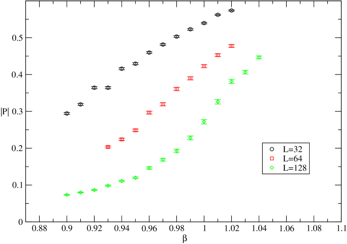
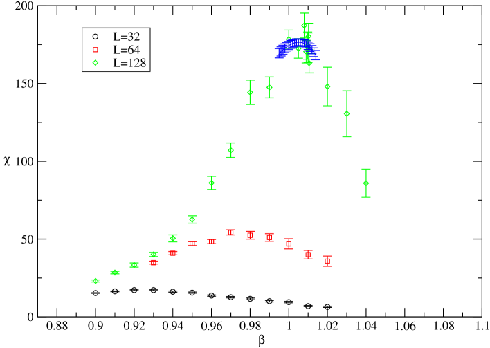
Figure 1: (Top) Absolute value of the Polyakov loop vs $\beta$ on a $1\times L^{2}$ lattice, with $L$=32, 64, 128. (Bottom) Susceptibility of the Polyakov loop vs $\beta$ on a $1\times L^{2}$ lattice, with $L$=32, 64, 128. For the $L$=128 case the multi-histogram interpolation around the peak is shown.

Table 2: $\beta_{pc}(L)$ for $N_{t}$=1, 4, 8 and for several values of $L$. Errors are determined by a jackknife analysis.

$L$	$N_{t}=1$	$N_{t}=4$	$N_{t}=8$
64	-	3.1250(51)	5.531(19)
128	1.0051(16)	-	5.754(22)
150	1.0094(26)	3.2190(40)	5.7945(59)
200	1.0227(15)	3.2368(39)	-
256	1.0278(20)	-	-

We determined $\beta_{c}(N_{t}=1)$ by fitting the pseudo-critical coupling $\beta_{pc}(L)$ given in the second column of Table 2 with the law

$$\beta_{pc}(L)=\beta_{c}+\frac{A}{(\log L)^{1/\nu}}\;,$$ (24)

in which $\nu$ was fixed by hand at the $XY$ value, $\nu=1/2$. We got $\beta_{c}(N_{t}=1)=1.107(9)$ and $A(N_{t}=1)=-2.4(2)$ ($\chi^{2}$/d.o.f.=0.78), which is quite in agreement with the best known $XY$ critical coupling, $\beta_{c}=1.1199(1)$, given in Ref. [11].

The determination of $\beta_{c}$ is crucial in order to extract critical indices; indeed, they enter scaling laws which hold just at $\beta_{c}$, such as, for example,

$$\chi(\beta_{c})\sim L^{2-\eta_{c}}\quad,$$ (25)

where $\eta_{c}$ is the magnetic critical index. Actually in Eq. 25 one should consider logarithmic corrections (see [12, 13] and references therein) and, indeed, recent works on the $XY$ universality class generally include them. However, taking these corrections into account for extracting critical indices calls for very large lattices even in the $XY$ model; for the theory under consideration to be computationally tractable, we have no choice but to neglect logarithmic corrections.

We determined $\chi(\beta=1.12)$ for $L$=64, 128, 150, 200, 256 – see Table 3 for a summary of the results. Fitting with the law (25), we found $\eta_{c}=0.256(29)$ ($\chi^{2}$/d.o.f.=0.2), in nice agreement with the $XY$ value, $\eta_{c}=1/4$. The same analysis repeated at $\beta=1.107$, i.e. at the central value of our determination of $\beta_{c}$, on lattices with $L$=64, 128, 200, gave $\eta_{c}=0.237(61)$ ($\chi^{2}$/d.o.f.=0.01).

An alternative strategy to determine $\eta_{c}$ uses the large distance behavior of the point-point correlator of the Polyakov loop,

$$C(R)=\sum_{x,n}\Re{\bigg{(}P_{x}^{\dagger}P_{x+R\cdot e_{n}}\bigg{)}}\quad,$$ (26)

where $e_{n}$ is the unit vector in the $n$-th direction. Without logarithmic corrections, one has

$$C(R)\sim\frac{1}{R^{\eta_{c}}}\quad.$$ (27)

In Fig. 2 we plot $\log C(R)$ vs $\log R$ for $L$=200 at $\beta=1.12$; linearity is clear up to $R\simeq 30$. Deviations at larger distances are due to finite size effects (echo terms are expected to be strong, since the correlator is long-ranged) and possibly to logarithmic corrections. In the linear regime ($5<R<30$), the naive fit with a power law gives $\eta$= 0.22942(31) ($\chi^{2}$/d.o.f.=0.83). The same analysis at $\beta=1.107$ and $L$=200 gives $\eta$= 0.2380(20) ($\chi^{2}$/d.o.f.=0.05) in the range $1<R<45$. On the same volume one sees that, for lower $\beta$’s, $\eta$ goes towards the expected value and that the linear region gets wider and wider.

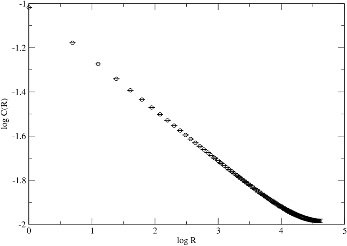
Figure 2: Log-log plot of point-point correlator for $L$=200 at $\beta=1.12$.

The effective $\eta_{c}$ index, defined as

$$\eta_{\mbox{\scriptsize eff}}(R)\equiv\frac{\log[C(R)/C(R_{0})]}{\log[R_{0}/R]}\quad,$$ (28)

must exhibit a plateau in the region where (27) holds. Fig. 3(top) shows that the larger the volume the larger the region in which there is a plateau at small distances. The chosen value of $R_{0}$ must belong to the linear region in order to minimize finite size effects. We have verified that varying $R_{0}$ in the linear region does not change the result and have chosen $R_{0}=10$ for all the cases considered here.

Since for the larger lattices ($L$=200 and $L$=256) plateaux are overlapping at small distances, one can conclude that thermodynamic limit is reached. We estimate the plateau value from the most precise data we have ($L$=200) as $\eta(\beta=1.12)=\eta_{\mbox{\scriptsize eff}}(R=6)=0.23101(49)$, since the latter is the value of $\eta_{\mbox{\scriptsize eff}}$ in the linear region compatible with the largest number of subsequent points. Deviations from the expected value $\eta$=0.25 can be due either to logarithmic corrections or to the overestimation of $\beta_{c}$. Repeating the same procedure for slightly lower $\beta$’s we find: $\eta(\beta=1.115)=0.23491(47)$ and $\eta(\beta=1.107)=0.24085(44)$. Notice that $\eta$ approaches the expected value as $\beta$ lowers. The relation between $\eta$ and $\beta$ is well described by a linear function ($\chi^{2}$/d.o.f.=0.04) and this suggests that the $\beta$ value at which $\eta$=0.25 is really close to those considered. Fig. 3(bottom) shows the correlation function $C(R)$ rescaled by $L^{-\eta}$ in units of $R/L$; it turns out that, when the best determination for $\eta$ is used (in the present case, $\eta=0.23101$) data from different lattices fall on top of each other over almost all the range of distances considered.

There are other observables which turned out to be useful in establishing the BKT scaling in the $2d$ $XY$ model and which we do not use in the present work: the helicity modulus ${\cal Y}$ [14, 13], the second moment correlation length $\xi_{2}$ (see, for instance, [13]) and the $U_{4}$ cumulant, proposed in [15]. We plan to use them all when we will study the general case $\beta_{s}\neq 0$. For the purposes of the present work we have only tried to use the $U_{4}$ cumulant, but both lattice sizes and statistics seem to be not enough large to extract any useful information from this observable.

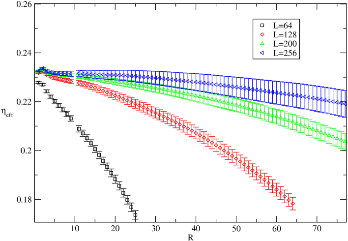
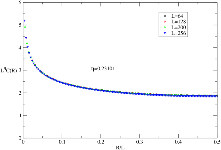
Figure 3: (Top) $\eta_{\mbox{\scriptsize eff}}$ for $N_{t}=1$ on lattices with several spatial sizes $L$ at $\beta=1.12$. For all lattices we fixed $R_{0}$=10. Errors are calculated with the jackknife method. (Bottom) $L^{\eta}C(R)$ versus $R/L$, with $\eta$ fixed at the central value of our determination through the method of the effective $\eta_{\mbox{\scriptsize eff}}$ (see the text).

4.2 $N_{t}$=4 and 8

In this Subsection we extend the study performed in the $N_{t}=1$ case to the cases of $N_{t}=4$ and 8, with the aim of showing that the universal $XY$ features are not lost increasing $N_{t}$ at $\beta_{s}$=0.

In Table 2 we give the values of the pseudo-critical couplings $\beta_{pc}(L)$ obtained from the peaks of the Polyakov loop susceptibility for several values of $L$ at $N_{t}=4$ and 8. Fitting these values with the law (24) with $\nu$ = 1/2 fixed, we get

$$\beta_{c}(N_{t}=4) = 3.42(1)\;,\;\;\;\;\;A(N_{t}=4)=-5.1(3)\;,\;\;\;\;\;(\chi^{2}/\mbox{d.o.f.}=0.43)$$

$$\beta_{c}(N_{t}=8) = 6.38(5)\;,\;\;\;\;\;A(N_{t}=8)=-15(1)\;,\;\;\;\;\;(\chi^{2}/\mbox{d.o.f.}=0.006)\quad.$$ (29)

This result shows that essential scaling is satisfied, i.e. in both cases transition is compatible with BKT. It is worth noting that these values of $\beta_{c}$ are in nice agreement with the estimates given in Table 1. This suggests that the dynamics of the effective model near the transition point is indeed dominated by the lower representations, thus justifying the truncation of the series in Eq. (20).

Table 3: $\chi(L)$ for $N_{t}$=1, 4, 8. Errors are determined by a jackknife analysis.

$L$	$N_{t}=1$	$N_{t}=4$	$N_{t}=8$
64	7.19(12)	9.30(57)	7.33(37)
128	24.6(1.3)	35.9(4.4)	25.1(1.5)
150	32.9(1.9)	42.5(2.5)	32.5(1.9)
200	51.4(2.7)	65.2(2.8)	58.4(3.3)
256	80.3(4.2)	101.7(5.4)	86.4(3.6)

In Table 3 we give the values of the Polyakov loop susceptibility for several values of $L$ at $\beta=3.42$ for $N_{t}=4$ and at $\beta=6.38$ for $N_{t}=8$. Fitting with (25), we find

$$\eta_{c}(N_{t}=4) = 0.290(54)\quad(\chi^{2}/\mbox{d.o.f.}=0.69)$$

$$\eta_{c}(N_{t}=8) = 0.212(46)\quad(\chi^{2}/\mbox{d.o.f.}=0.28)\quad.$$ (30)

Results agree with the universal $XY$ value $\eta_{c}=1/4$, although errors are quite large.

A more precise determination of the magnetic index can be achieved through the study of the point-point correlation function. In Figs. 4(top) and 5(top) we show $\eta_{\mbox{\scriptsize eff}}(R)$ for three values of the spatial size $L$ for the cases of $N_{t}=4$ and $N_{t}=8$, respectively. Our estimated plateau values, taken from data at $L=200$, are

$$\eta(\beta=3.42) = \eta_{\mbox{\scriptsize eff}}(N_{t}=4,R=2)=0.2724(11)\;,$$

$$\eta(\beta=6.38) = \eta_{\mbox{\scriptsize eff}}(N_{t}=8,R=3)=0.2499(11)\;.$$

For $N_{t}=4$, $\eta$ overshoots by little the $XY$ universal value, while for $N_{t}=8$ it is in nice accord with it. The deviation for $N_{t}=4$ is most likely washed out by a fine tuning of the critical coupling within its error bars.

One can observe, moreover, that the shape of the curve of values of $\eta_{\mbox{\scriptsize eff}}(R)$ changes qualitatively in the same way when the thermodynamic limit is approached for $N_{t}=1$ and $N_{t}=8$, while it has a different behavior for $N_{t}=4$. This may be an indication that for $N_{t}=1$ and $N_{t}=8$ at the $\beta$’s chosen for the simulation the system is in the same phase ($\beta>\beta_{c}$), i.e. correlators have the same behavior.

Figs. 4(bottom) and  5(bottom) show the correlation function $C(R)$ rescaled by $L^{-\eta}$ in units of $R/L$, with $\eta$ fixed at the central value of our determinations ($\eta=0.2724$ for $N_{t}=4$ and $\eta=0.2499$ for $N_{t}=8$); one can see that data from different lattices fall on top of each other over a wide range of distances.

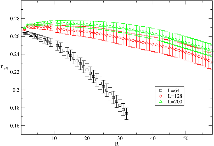
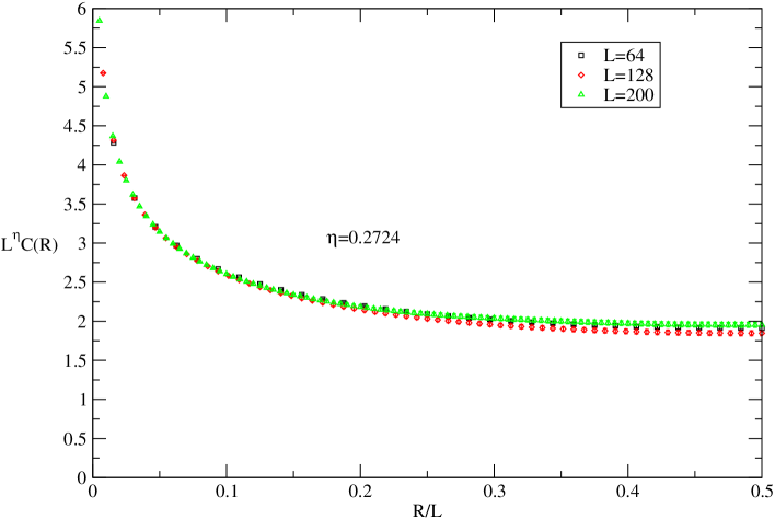
Figure 4: (Top) $\eta_{\mbox{\scriptsize eff}}$ for $N_{t}=4$ on lattices with $L$=64, 128, 200 at $\beta=3.42$. For all lattices we fixed $R_{0}$=10. Errors are determined by the jackknife method. (Bottom) $L^{\eta}C(R)$ versus $R/L$, with $\eta$ fixed at the central value of our determination through the method of the effective $\eta_{\mbox{\scriptsize eff}}$ (see the text).

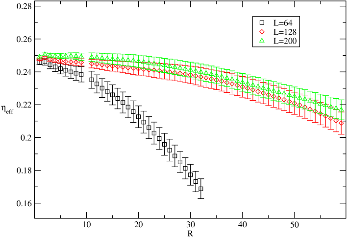
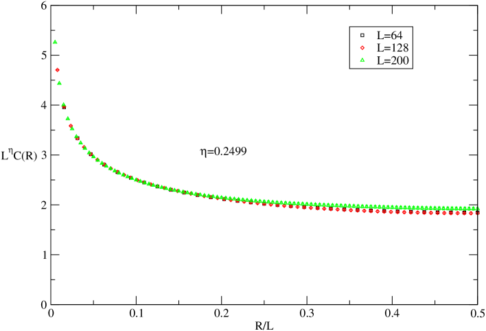
Figure 5: (Top) $\eta_{\mbox{\scriptsize eff}}$ for $N_{t}=8$ on lattices with $L$=64, 128, 200 at $\beta=6.38$. For all lattices we fixed $R_{0}$=10. Errors are determined by the jackknife method. (Bottom) $L^{\eta}C(R)$ versus $R/L$, with $\eta$ fixed at the central value of our determination through the method of the effective $\eta_{\mbox{\scriptsize eff}}$ (see the text).

In summary, essential scaling is verified both for $N_{t}=4$ and 8, thus indicating that indeed the occurring transitions are compatible with BKT. Moreover data point to values of the thermal and magnetic critical indices of the 2$d$ $XY$ universality class. This leads us to conclude that for $N_{t}=4$ and 8 the 3$d$ U(1) LGT at $\beta_{s}$=0 belongs to the 2$d$ $XY$ universality class and this supports the conjecture that the same holds, in general, for any $N_{t}$ at $\beta_{s}=0.$

Since we do not study the correlation length, we are not allowed to rule out the possibility that it keeps finite and the transition is therefore first order. To this aim, we have performed a fit to the pseudo-critical couplings with the first order law

$$\beta_{pc}(L)=\beta_{c}+\frac{B}{L^{2}}\;,$$ (31)

finding

$$\beta_{c}(N_{t}=4) = 3.245(3)\;,\;\;\;\;\;B(N_{t}=4)=-500(30)\;,\;\;\;\;\;(\chi^{2}/\mbox{d.o.f.}=2.1)$$

$$\beta_{c}(N_{t}=8) = 5.852(8)\;,\;\;\;\;\;B(N_{t}=8)=-1300(100)\;,\;\;\;\;\;(\chi^{2}/\mbox{d.o.f.}=0.6)\quad.$$ (32)

Looking at the $\chi^{2}$/d.o.f., one can argue that for $N_{t}=4$ first order should be ruled out, whereas $N_{t}=8$ is compatible with first order scaling.  This can be due to the limited volumes ($L\leq 150$) considered for $N_{t}=8$ and to the larger error bars in the determinations of the $\beta_{pc}$’s with respect to the $N_{t}=4$ case. However, for $N_{t}=8$ the good agreement between the numerical result for the magnetic critical index and the corresponding value in the $2d$ $XY$ model supports the claim that, even for this $N_{t}$, the transition is BKT.

5 Conclusions and outlook

The purpose of this paper has been to study the critical behavior of 3$d$ U(1) LGT at finite temperatures, through the formulation on an asymmetric lattice. While the theory at zero-temperature is always in the confined phase, at finite temperatures it undergoes a deconfinement phase transition, just as it happens for 4$d$ QCD. Analytical results from the high-temperature expansion suggest that this transition is of BKT type, but compelling numerical evidence is missing that indeed critical indices of 3$d$ U(1) LGT coincide with those of the 2$d$ $XY$ model.

This paper is the first step in the construction of the phase diagram of 3$d$ U(1) LGT in the $(\beta_{t},\beta_{s})$-plane, where $\beta_{s}$ ($\beta_{t})$ is the spatial (temporal) coupling. In particular, we restricted ourselves to the case $\beta_{s}=0$ and, by means of numerical Monte Carlo simulations on a dimensionally reduced effective theory, found evidence that the theory belongs indeed to the same universality class of the 2$d$ $XY$ model. The key observations have been the appearance of essential scaling and the agreement of the magnetic critical index $\eta$ with that from the 2$d$ $XY$ model.

The next step is the extension of the numerical procedure established in this paper to the general case of $\beta_{s}\neq 0$.

Acknowledgment

O.B. thanks for warm hospitality the Dipartimento di Fisica dell’Università della Calabria and the INFN Gruppo Collegato di Cosenza, where the idea of this investigation came up. A.P. is grateful to the Department of Nuclear Physics of the Technical University of Vienna for hosting him during the final stages of the work.

References

- [1] M. N. Chernodub, E. M. Ilgenfritz, A. Schiller, Phys. Rev. D 64 (2001) 054507; Phys. Rev. Lett. 88 (2002) 231601; Phys. Rev. D 67 (2003) 034502.
- [2] A. Polyakov, Nucl. Phys. B 120 (1977) 429; M. Göpfert, G. Mack, Commun. Math. Phys. 81 (1981) 97; 82 (1982) 545.
- [3] N. Parga, Phys. Lett. B 107 (1981) 442.
- [4] B. Svetitsky, L. Yaffe, Nucl. Phys B 210 (1982) 423.
- [5] V. L. Berezinsky, Sov. Phys. JETP 32 (1971) 493.
- [6] J. M. Kosterlitz and D. J. Thouless, J. Phys. C 6 (1973) 1181.
- [7] P. D. Coddington, A. J. G. Hey, A. A. Middleton and J. S. Townsend, Phys. Lett. B 175 (1986) 64.
- [8] R. Kenna, The model and the Berezinskii-Kosterlitz-Thouless phase transition, arXiv:cond-mat/0512356.
- [9] A. C. D. van Enter and S. B. Shlosman, Phys. Rev. Lett. 89 (2002) 285702.
- [10] A. M. Ferrenberg and R. H. Swendsen, Phys. Rev. Lett. 63 (1989) 1195.
- [11] M. Hasenbusch and K. Pinn, J. Phys. A 30 (1997) 63.
- [12] R. Kenna and A. C. Irving, Nucl. Phys. B 485 (1997) 583.
- [13] M. Hasenbusch, J. Phys. A 38 (2005) 5869.
- [14] H. Weber and P. Minnhagen, Phys. Rev. B 37 (1988) 5986.
- [15] M. Hasenbusch, arXiv:cond-mat/0804.1880.