Semitoric integrable systems on symplectic $4$-manifolds

Abstract

Let $(M,\,\omega)$ be a symplectic $4$-manifold. A semitoric integrable system on $(M,\,\omega)$ is a pair of smooth functions $J,\,H\in\!\!\mathop{\rm~{}C}\nolimits^{\infty}(M,\,{\mathbb{R}})$ for which $J$ generates a Hamiltonian $S^{1}$-action and the Poisson brackets $\{J,\,H\}$ vanish. We shall introduce new global symplectic invariants for these systems; some of these invariants encode topological or geometric aspects, while others encode analytical information about the singularities and how they stand with respect to the system. Our goal is to prove that a semitoric system is completely determined by the invariants we introduce.

1 Introduction

Atiyah [1, Th. 1] and Guillemin-Sternberg [9] proved that the image $\mu(M)$ under the momentum map $\mu:=(\mu_{1},\ldots,\mu_{n})\colon M\to{\mathbb{R}}^{n}$ of a Hamiltonian action of an $n$-dimensional torus on a compact connected symplectic manifold $(M,\,\omega)$ is a convex polytope, called the momentum polytope. Delzant [3] showed that if the dimension of the torus is half the dimension of $M$, the momentum polytope, which in this case is called Delzant polytope, determines the isomorphism type of $M$. Moreover, he showed that $M$ is a toric variety. These theorems establish remarkable and deep connections bewteen Hamiltonian dynamics, symplectic geometry, Kähler manifolds and toric varieties in algebraic geometry. Through the analysis of the quantization of such systems, one may also mention important links with the representation theory of Lie groups and Lie algebras, semiclassics, and microlocal analysis.

Nevertheless, at least from the viewpoint of symplectic geometry, the situation described by the momentum polytope is very rigid. There are at least three natural directions for further mathematical exploration : (i) replacing the manifold $M$ by an orbifold; (ii) allowing more general actions than Hamiltonian ones, (iii) replacing the torus $T$ by a non-abelian and/or non-compact Lie group $G$.

Following (i) Lerman-Tolman generalized Delzant’s classification to orbifolds in [13, Th. 7.4, 8.1]. Regarding (i) Pelayo generalized Delzant’s result to the case when $M$ is $4$-dimensional and $T$ acts symplectically, but not necessarily Hamiltonianly [18, Th. 8.2.1]. This result relies on the generalization of Delzant’s theorem for symplectic torus actions with coisotropic principal orbits by Duistermaat-Pelayo earlier [5, Th. 9.4, 9.6], and for symplectic torus actions with symplectic principal orbits by Pelayo [18, Th. 7.4.1]. Regarding (iii), results for non-abelian compact Lie groups $G$ are relatively complete, see Kirwan [11], Lerman-Meinrenken-Tolman-Woodward [14], Sjamaar [20] and Guillemin-Sjamaar [8]. When $T$ is replaced by a non-compact group $G$ the theory is hard; even in the proper and Hamiltonian case, the symplectic local normal form for a proper action requires extensive work, see Marle [15] and Guillemin-Sternberg [10, Sec. 41]; in the non-Hamiltonian symplectic case this normal form is recent work of Benoist [2, Prop. 1.9] and Ortega-Ratiu [17].

The seemingly most simple non-compact case to study is that of a Hamiltonian action of the abelian group ${\mathbb{R}}^{n}$ on a $2n$-dimensional symplectic manifold. But of course, this is nothing less than the goal of the theory of integrable systems. The role of the momentum map is in this case played by a map of the form $F:=(f_{1},\,\dots,\,f_{n})\colon M\to{\mathbb{R}}^{n},$ where $f_{i}\colon M\to{\mathbb{R}}$ is smooth, the Poisson brackets $\{f_{i},\,f_{j}\}$ identically vanish on $M$, and the differentials $\!\mathop{\rm d\!}\nolimits{}f_{1},\,\dots,\,\!\mathop{\rm d\!}\nolimits{}f_{n}$ are almost-everywhere linearly independent. In this article we study the case of an integrable system $f_{1}:=J,\,f_{2}:=H$, where $M$ is $4$-dimensional and the component $J$ generates a Hamiltonian $S^{1}$-action: these are called semitoric. Semitoric systems form an important class of integrable systems, commonly found in simple physical models. Indeed, a semitoric system can be viewed as a Hamiltonian system in the presence of an $S^{1}$ symmetry [19]. One of the incentives for this work is that it is much simpler to understand the integrable system on its whole rather than writing a theory of Hamiltonian systems on Hamiltonian $S^{1}$-manifolds.

It is well established in the integrable systems community that the most simple and natural object, which tells much about the structure of the integrable system under study, is the so-called bifurcation diagram. This is nothing but the image in ${\mathbb{R}}^{2}$ of $F=(J,\,H)$ or, more precisely, the set of critical values of $F$. In this article, we are going to show that the arrangement of such critical values is indeed important, but other crucial ingredients are needed to understand $F$, which are more subtle and cannot be detected from the bifurcation diagram itself. Our goal is to construct a collection of new global symplectic invariants for semitoric integrable systems which completely determine a semitoric system up to isomorphisms. We will build on a number of remarkable results by other authors in integrable systems, including Arnold, Atiyah, Dufour-Molino, Eliasson, Duistermaat, Guillemin-Sternberg, Miranda-Zung and Vũ Ngọc, to which we shall make references throughout the text, and to whom this paper owes much credit.

The paper is structured as follows; in Section 2 we define semitoric systems, explain the conditions which appear in the definition and announce our main result; in sections 3,4 and 5 we construct the new symplectic invariants. Specifically, in Section 3 we study the analytical invariants, in Section 4 we study the combinatorial invariants, and in Section 5 we study the geometric invariants. In Section 6 we state the aforementioned theorem, which we prove in Section 7. The paper concludes with a short appendix, Section 8, in which we prove a very slight modification of a result of Miranda-Zung which we need earlier.

2 Semitoric systems

First we introduce the precise definition of semitoric integrable system.

Definition 2.1   Let $(M,\,\omega)$ be a connected symplectic $4$-dimensional manifold. A semitoric integrable system on $M$ is an integrable system $J,\,H\in\!\!\mathop{\rm~{}C}\nolimits^{\infty}(M,\,{\mathbb{R}})$ for which

• the component $J$ is a proper momentum map for a Hamiltonian circle action on $M$;

• the map $F:=(J,\,H):M\to{\mathbb{R}}^{2}$ has only non-degenerate singularities in the sense of Williamson, without real-hyperbolic blocks.

We also use the terminology $4$-dimensional semitoric integrable system to refer to the triple $(M,\,\omega,\,(J,\,H))$. $\oslash$

We recall that the first point in Definition 2 means that the preimage by $J$ of a compact set is compact in $M$ (which is of course automatic if $M$ is compact), and the second point means that, whenever $m$ is a critical point of $F$, there exists a 2 by 2 matrix $B$ such that, if we denote $\tilde{F}=B\circ F$, one of the following happens, in some local symplectic coordinates near $m$ :

• $\tilde{F}(x,\,y,\,\xi,\,\eta)=(\eta+\mathcal{O}(\eta^{2}),\,x^{2}+\xi^{2}+\mathcal{O}((x,\,\xi)^{3}))$

• $\!\!\mathop{\rm~{}d}\nolimits^{2}_{m}\tilde{F}(x,\,y,\,\xi,\,\eta)=(x^{2}+\xi^{2},\,y^{2}+\eta^{2})$

• $\!\!\mathop{\rm~{}d}\nolimits^{2}_{m}\tilde{F}(x,\,y,\,\xi,\,\eta)=(x\xi+y\eta,\,x\eta-y\xi)$

The first case is called a transversally — or codimension 1 — elliptic singularity; the second case is an elliptic-elliptic singularity; the last case is a focus-focus singularity.

In [22], Vũ Ngọc proved a version of the Atiyah-Guillemin-Sternberg theorem: to a $4$-dimensional semitoric integrable system one may meaningfully associate a family of convex polygons which generalizes the momentum polygon that one has in the presence of a Hamiltonian $2$-torus action. If two such systems are isomorphic, then these two families of polygons are equal.

In view of this, a natural goal is to try to understand whether a semitoric integrable system on a symplectic $4$-manifold could possibly be determined by this family of polygons; as it turns out this is one of five invariants we associate to such a system. Precisely, the invariants are the following: (i) the number of singularities invariant: an integer counting the number of isolated singularities; (ii) the singularity type invariant: which classifies locally the type of singularity; (iii) the polygon invariant: a family of weighted rational convex polygons (generalizing the Delzant polygon and which may be viewed as a bifurcation diagram); (iv) the volume invariant: numbers measuring volumes of certain submanifolds at the singularities; (v) the twisting index invariant: integers measuring how twisted the system is around singularities. Our goal in this paper is to prove an integrable system is completely determined, up to isomorphisms, by these invariants. In other words, we shall prove that:

$(M,\,\omega_{1},\,(J_{1},\,H_{1}))$ and $(M,\,\omega_{2},\,(J_{2},\,H_{2}))$ are isomorphic $\iff$ they have the same invariants (i)–(v).

Here the word isomorphism is used in the sense that there exists a symplectomorphism

$$\varphi\colon M_{1}\to M_{2},\,\,\,\,\,\,\,\textup{such that}\,\,\,\,\,\varphi^{*}(J_{2},\,H_{2})=(J_{1},\,f(J_{1},\,H_{1})).$$

for some smooth function $f$ (see Theorem 6.2).

One could say that (i) and (ii) are analytical invariants, (iii) is a combinatorial/group-theoretic invariant, and (iv), (v) are geometric invariants.

3 Analytic invariants of a semitoric system

We describe invariants of a semitoric system encoding analytic information about the singularities. Throughout this section $(M,\,\omega,\,(J,\,H))$ is a $4$-dimensional semitoric integrable system.

3.1 Cardinality of singular set invariant

It is clear from the definition that a semitoric integrable system has only two types of singularities: elliptic (of codimension $0$ or $1$) and focus-focus. This can easily be inferred from the bifurcation diagram. In fact, Vũ Ngọc proves in [22, Prop. 2.9, Th. 3.4, Cor. 5.10] the following statement :

Proposition 3.1.

The semitoric system $(M,\,\omega,\,(J,\,H))$ admits a finite number $m_{f}$ of focus-focus critical values $c_{1},\dots,c_{m_{f}}$, and, denoting by $B=F(M)$ the image of $F$, where $F=(J,\,H)$:

• the set of regular values of $F$ is $B_{r}=\!\!\mathop{\rm~{}Int}\nolimits{B}\setminus\{c_{1},\dots,c_{m_{f}}\};$

• the boundary of $B$ consists of all images of elliptic singularities;

• the fibers of $F$ are connected.

Of course $m_{f}$ is an invariant of the singular foliation induced by $F$, where $m_{f}$ and $F$ are as in Proposition 3.1. Since this foliation is preserved by isomorphism, we have the following result.

Lemma 3.2.

Let $(M_{1},\,\omega_{1},(J_{1},\,H_{1})),\,(M_{2},\,\omega_{2},(J_{2},\,H_{2}))$ be isomorphic $4$-dimensional semitoric integrable systems and let $m_{f}^{i}$ be the number of focus-focus points of $(M_{i},\,\omega_{i},(J_{i},\,H_{i}))$, where $i\in\{1,\,2\}$. Then $m^{1}_{f}=m^{2}_{f}$.

One may argue that $m_{f}$ is a combinatorial invariant, since it is an integer; we have put it in this section because we need it for the construction of the true analytic invariant of the system, defined in Section 3.2: the singularity type invariant.

3.2 Singularity type invariant

Let $F$, $m_{f}$ and $c_{1},\ldots,c_{m_{f}}$ be as in Proposition 3.1 We consider here the preimage by $F$ of a focus-focus critical value $c_{i}$, where $i\in\{1,\,\ldots,\,m_{f}\}$. Throughout, we will assume that the critical fiber

$$\mathcal{F}_{m}:=F^{-1}(c_{i})$$

contains only one critical point $m$. According to Zung [23], this is a genericity assumption.

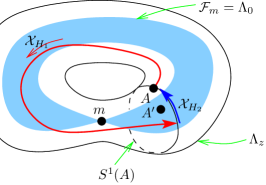
Figure 3.1: The singular foliation $\mathcal{F}$ associated to $F$ near the singular leaf $\mathcal{F}_{m}$, where $S^{1}(A)$ denotes the $S^{1}$-orbit for the $S^{1}$-action generated by $H_{2}$.

Let $\mathcal{F}$ denote the associated singular foliation. Eliasson’s theorem [7] describes a neighborhood $U$ of a focus-focus point $m$ in a singular foliation of focus-focus type: there exist symplectic coordinates $(x,\,y,\,\xi,\,\eta)$ in $U$ in which the map $(q_{1},\,q_{2})$, given by

$$q_{1}=x\xi+y\eta,\qquad q_{2}=x\eta-y\xi,$$ (3.1)

is a momentum map for the foliation $\mathcal{F}$; here the critical point $m$ corresponds to coordinates $(0,\,0,\,0,\,0)$. Let us fix a point $A^{\prime}\in\mathcal{F}_{m}\cap(U\setminus\{m\})$, let $\Sigma$ denote a small 2-dimensional surface transversal to $\mathcal{F}$ at the point $A^{\prime}$, and let $\Omega$ be the open neighborhood of the leaf $\mathcal{F}_{m}$ which consists of the leaves which intersect the surface $\Sigma$.

Since the Liouville foliation in a small neighborhood of $\Sigma$ is regular for both momentum maps $F$ and $q=(q_{1},\,q_{2})$, there must be a local diffeomorphism $\varphi$ of ${\mathbb{R}}^{2}$ such that $q=\varphi\circ{F}$, and hence we can define a global momentum map $\Phi=\varphi\circ{F}$ for the foliation, which agrees with $q$ on $U$. Write $\Phi:=(H_{1},\,H_{2})$ and $\Lambda_{z}:=\Phi^{-1}(z)$. Note that $\Lambda_{0}=\mathcal{F}_{m}.$ It follows from (3.1) that near $m$ the $H_{2}$-orbits must be periodic of primitive period $2\pi$ for any point in a (non-trivial) trajectory of $\mathcal{X}_{H_{1}}$.

Suppose that $A\in\Lambda_{z}$ for some regular value $z$. We define $\tau_{1}(z)$, which is a strictly positive number, as the time it takes the Hamiltonian flow associated to $H_{1}$ leaving from $A$ to meet the Hamiltonian flow associated to $H_{2}$ which passes through $A$, and let $\tau_{2}(z)\in{\mathbb{R}}/2\pi{\mathbb{Z}}$ the time that it takes to go from this intersection point back to $A$, hence closing the trajectory. Write $z=(z_{1},\,z_{2})=z_{1}+\!\!\mathop{\rm~{}i}\nolimits z_{2}$, and let $\!\!\mathop{\rm~{}ln}\nolimits z$ for a fixed determination of the logarithmic function on the complex plane. We moreover define the following two functions:

$$\left\{\begin{array}[]{ccl}\sigma_{1}(z)&=&\tau_{1}(z)+\Re(\!\!\mathop{\rm~{}ln}\nolimits z)\\ \sigma_{2}(z)&=&\tau_{2}(z)-\Im(\!\!\mathop{\rm~{}ln}\nolimits z),\end{array}\right.$$ (3.2)

where $\Re$ and $\Im$ respectively stand for the real an imaginary parts of a complex number. In his article [21, Prop. 3.1], Vũ Ngọc proved that $\sigma_{1}$ and $\sigma_{2}$ extend to smooth and single-valued functions in a neighbourhood of $0$ and that the differential 1-form

$$\sigma:=\sigma_{1}\,\!\mathop{\rm d\!}\nolimits{}z_{1}+\sigma_{2}\,\!\mathop{\rm d\!}\nolimits{}z_{2}$$ (3.3)

is closed. Notice that if follows from the smoothness of $\sigma_{2}$ that one may choose the lift of $\tau_{2}$ to ${\mathbb{R}}$ such that $\sigma_{2}(0)\in[0,\,2\pi)$. This is the convention used throughout.

Definition 3.3  [21, Def. 3.1] Let $S_{i}$ be the unique smooth function defined around $0\in{\mathbb{R}}^{2}$ such that

$$\left\{\begin{array}[]{rl}\!\mathop{\rm d\!}\nolimits{}S_{i}=\sigma\\ S_{i}(0)=0\end{array}\right.,$$ (3.6)

where $\sigma$ is the one-form given by (3.3). The Taylor expansion of $S$ at $(0,\,0)$ is denoted by $(S)^{\infty}$. We say that $(S_{i})^{\infty}$ is the Taylor series invariant of $(M,\,\omega,\,(J,\,H))$ at the focus-focus point $c_{i}$, where $i\in\{1,\,\ldots,\,m_{f}\}$. $\oslash$

The Taylor expansion $(S)^{\infty}$ is a formal power series in two variables with vanishing constant term.

Lemma 3.4.

Let $(M_{1},\,\omega_{1},(J_{1},\,H_{1})),\,(M_{2},\,\omega_{2},(J_{2},\,H_{2}))$ be isomorphic $4$-dimensional semitoric integrable systems and let $((S^{j}_{i})^{\infty})_{i=1}^{m^{i}_{f}}$ be the tuple of Taylor series invariants at the focus-focus critical points of $(M_{j},\,\omega_{j},(J_{j},\,H_{j}))$, where $j\in\{1,\,2\}$. Then the tuple $((S^{1}_{i})^{\infty})_{i=1}^{m^{1}_{f}}$ is equal to the tuple $((S^{2}_{i})^{\infty})_{i=1}^{m^{2}_{f}}$.

This result was proven in [22].

4 Combinatorial invariants of a semitoric system

The Atiyah-Guillemin-Sternberg and Delzant theorems tell us that a lot of the information of some completely integrable systems coming from Hamiltonian torus actions is encoded combinatorially by polytopes.

Figure 4.1: Momentum polytope of $\mathbb{CP}^{2}$ (left), a Hirzebruch surface (center) and $(\mathbb{CP}^{1})^{2}$ (right), all of which determine the isomorphism type of the manifold.

Although $4$-dimensional semitoric systems are not induced by torus actions, some of the information of the system may be combinatorially encoded by a certain equivalence class of rational convex polygons endowed with a collection of vertical weighted lines. This is in fact a way of encoding the affine structure induced by the integrable system. Throughout this section $(M,\,\omega,\,(J,\,H))$ is a $4$-dimensional semitoric integrable system with $m_{f}$ isolated focus-focus singular values.

4.1 Affine Structures

Recall that a map $X\subset\mathbb{R}^{m}\to Y\subset\mathbb{R}^{m}$ is integral-affine on $X$ if it is of the form $A_{ij}(\cdot)+b_{ij},$ where $A_{ij}\in\textup{GL}(m,\,\mathbb{Z})$ and $b_{ij}\in\mathbb{R}^{m}$.

An integral-affine smooth $m$-dimensional manifold is a smooth $m$-dimensional manifold $X$ for which the coordinate changes are integral-affine, i.e. if $\varphi_{i}\colon U_{i}\subset\mathbb{R}^{m}\to X$ are the charts associated to $X$, for all $i,\,j$ we have that $\varphi_{i}\circ\varphi_{j}^{-1}$, whereever defined, is an integral affine map. We allow manifolds with boundary and corners, in which case the charts take their values in $[0,+\infty)^{k}\times{\mathbb{R}}^{m-k}$ for some integer $k\in\{0,\dots,m\}$.

A map $f\colon X\to Y$ between integral affine manifolds is integral-affine if for each point $x\in X$ there are charts $\varphi_{x}\colon U_{x}\to X$ around $x$ and $\psi_{y}\colon V_{y}\to Y$ around $y:=f(x)$ such that $\psi_{y}^{-1}\circ f\circ\varphi_{x}$ is integral-affine.

Any Lagrangian fibration $F:M\to B$ naturally defines an integral-affine structure on the base $B$. This affine structure can be characterized by the following fact : a local diffeomorphism $g:(B,\,b)\to({\mathbb{R}}^{n},\,0)$ is integral-affine if and only if the Hamiltonian flows of the $n$ coordinate functions of $g\circ F$ are periodic of primitive period equal to $2\pi$. Thus, an integrable system with momentum map $F=(J,\,H)$ defines an integral-affine structure on the set $B_{r}$ of regular values of $F$. In our case, this structure will in fact extend to the boundary of $B_{r}$. Although $B_{r}$ is a subset of ${\mathbb{R}}^{2}$, the integral-affine structure of $B_{r}$ is in general different from the induced canonical integral-affine structure of ${\mathbb{R}}^{2}$.

The integral-affine structure of $B_{r}$ encodes much of the topology of the integrable system (see [23]) but, as we will see, is far from encoding all its symplectic geometry.

4.2 Generalized toric map

We start with two definitions that we shall need. Let $\mathfrak{I}$ be the subgroup of the affine group $\!\!\mathop{\rm~{}Aff}\nolimits(2,\,{\mathbb{Z}})$ in dimension 2 of those transformations which leave a vertical line invariant, or equivalently, an element of $\mathfrak{I}$ is a vertical translation composed with a matrix $T^{k}$, where $k\in{\mathbb{Z}}$ and

$$T^{k}:=\left(\begin{array}[]{cc}1&0\\ k&1\end{array}\right)\in\!\!\mathop{\rm~{}GL}\nolimits(2,\,{\mathbb{Z}}).$$ (4.3)

Let $\ell\subset{\mathbb{R}}^{2}$ be a vertical line in the plane, not necessarily through the origin, which splits it into two half-spaces, and let $n\in{\mathbb{Z}}$. Fix an origin in $\ell$. Let $\!\!\mathop{\rm~{}t}\nolimits^{n}_{\ell}\colon{\mathbb{R}}^{2}\to{\mathbb{R}}^{2}$ be the identity on the left half-space, and $T^{n}$ on the right half-space. By definition $\!\!\mathop{\rm~{}t}\nolimits^{n}_{\ell}$ is piecewise affine. Let $\ell_{i}$ be a vertical line through the focus-focus value $c_{i}=(x_{i},\,y_{i})$, where $1\leq i\leq m_{f}$, and for any tuple $\vec{n}:=(n_{1},\,\dots,\,n_{m_{f}})\in{\mathbb{Z}}^{m_{f}}$ we set

$$\!\!\mathop{\rm~{}t}\nolimits_{\vec{n}}:=\!\!\mathop{\rm~{}t}\nolimits^{n_{1}}_{\ell_{1}}\circ\,\cdots\,\circ\!\!\mathop{\rm~{}t}\nolimits^{n_{m_{f}}}_{\ell_{m_{f}}}.$$ (4.4)

The map $t_{\vec{n}}$ is piecewise affine.

In [22, Th. 3.8] Vũ Ngọc describes how to associate to $(M,\,\omega,\,F=(J,\,H))$ a rational convex polygon: the image of a certain almost everywhere integral-affine homeomorphism $f\colon F(M)\subset{\mathbb{R}}^{2}\to\Delta\subset{\mathbb{R}}^{2}$. Here, $B:=F(M)$ is equipped with the natural integral-affine structure induced by the system, while ${\mathbb{R}}^{2}$ on the right hand-side is endowed with its canonical integral-affine structure.

Given a sign $\epsilon_{i}\in\{-1,+1\}$, let $\ell_{i}^{\epsilon_{i}}\subset\ell_{i}$ be the vertical half line starting at $c_{i}$ at extending in the direction of $\epsilon_{i}$ : upwards if $\epsilon_{i}=1$, downwards if $\epsilon_{i}=-1$. Let

$$\ell^{\vec{\epsilon}}:=\bigcup_{i=1}^{m_{f}}\ell_{i}^{\epsilon_{i}}.$$

Theorem 4.1 (Th. 3.8 in [22]).

For $\vec{\epsilon}\in\{-1,+1\}^{m_{f}}$ there is a homeomorphism $f=f_{\epsilon}\colon B\to{\mathbb{R}}^{2}$ such that

1. $f|_{(B\setminus\ell^{\vec{\epsilon}})}$ is a diffeomorphism into its image $\Delta:=f(B)$.

2. $f|_{(B_{r}\setminus\ell^{\vec{\epsilon}})}$ is affine: it sends the integral affine structure of $B_{r}$ to the standard structure of ${\mathbb{R}}^{2}$.

3. $f$ preserves $J$: i.e. $f(x,\,y)=(x,\,f^{(2)}(x,\,y))$.

4. For any $i\in\{1,\,\ldots,\,m_{f}\}$ and any $c\in\ell_{i}^{\epsilon_{i}}\setminus\{c_{i}\}$ there is an open ball $D$ around $c$ such that $f|_{(B_{r}\setminus l^{\vec{\epsilon}})}$ has a smooth extension on each domain $\{(x,\,y)\in D\,\mid\,\leq x_{i}\}$ and $\{(x,\,y)\in D\,\mid\,x\geq x_{i}\}$. One has the formula:

   $$\lim_{\begin{subarray}{c}(x,y)\to c\\ x<x_{i}\end{subarray}}\!\!\mathop{\rm~{}d}\nolimits f(x,\,y)=T^{k(c)}\lim_{\begin{subarray}{c}(x,y)\to c\\ x>x_{i}\end{subarray}}\!\!\mathop{\rm~{}d}\nolimits f(x,\,y),$$

   where $k(c)$ is the multiplicity of $c$.

5. The image of $f$ is a rational convex polygon.

Such an $f$ is unique modulo a left composition by a transformation in $\mathfrak{I}$.

In order to arrive at the rational convex polygon $\Delta$ in the proof of Theorem 4.1 one cuts the image $(J,\,H)(M)\subset{\mathbb{R}}^{2}$, which is in general not convex, along each of the vertical lines $\ell_{i}$, $i\in\{1,\,\ldots,\,m_{f}\}$. One must make a choice of “cut direction” for each vertical line $\ell_{i}$, that is to say that one has to choose whether to cut the set $(J,\,H)(M)$ along the half-vertical-line $\ell_{i}^{+1}$ which starts at $c_{i}$ going upwards, or along the half-vertical-line $\ell_{i}^{-1}$ which starts at $c_{i}$ going downwards. Precisely, the definitions of $f$ and $\Delta$ in Theorem 4.1 depend on two choices in the proof :

• an initial set of action variables $f_{0}$ of the form $(J,\,K)$ near a regular Liouville torus in [22, Step 2, pf. of Th. 3.8]. If we choose $f_{1}$ instead of $f_{0}$ we get a polytope $\Delta^{\prime}$ by left composition with an element of $\mathfrak{I}$. Similarly instead instead of $f$ we obtain $f$ composed on the left with an element of $\mathfrak{I}$;

• a tuple $\vec{\epsilon}$ of $1$ and $-1$. If we choose $\vec{\epsilon^{\prime}}$ instead of $\vec{\epsilon}$ we get $\Delta^{\prime}=\!\!\mathop{\rm~{}t}\nolimits_{\vec{u}}(\Delta)$ with $u_{i}=(\epsilon_{i}-\epsilon^{\prime}_{i})/2$, by [22, Prop. 4.1, expr. (11)]. Similarly instead of $f$ we obtain $f^{\prime}=\!\!\mathop{\rm~{}t}\nolimits_{\vec{u}}\circ f$.

Definition 4.2   Let $(M,\,\omega,\,(J,\,H))$ be a semitoric integrable system and let $f$ a choice of homeomorphism as in Theorem 4.1. We say that:

• the map $f\circ(J,\,H)$ is a generalized toric momentum map for $(M,\,\omega,\,(J,\,H))$;

• the rational convex polygon $\Delta:=f\big{(}(J,\,H)(M)\big{)}$ is a a generalized toric momentum polygon for $(M,\,\omega,\,(J,\,H))$.

$\oslash$

For simplicity sometimes we omit the word “generalized” in Definition 4.1.

4.3 Semitoric polygon invariant

Let $\!\!\mathop{\rm~{}Polyg}\nolimits({\mathbb{R}}^{2})$ be the space of rational convex polygons in ${\mathbb{R}}^{2}$. Let $\!\!\mathop{\rm~{}Vert}\nolimits({\mathbb{R}}^{2})$ be the set of vertical lines in ${\mathbb{R}}^{2}$, i.e.

$$\!\!\mathop{\rm~{}Vert}\nolimits({\mathbb{R}}^{2})=\Big{\{}\ell_{\lambda}:=\{(x,\,y)\in{\mathbb{R}}^{2}\,|\,x=\lambda\}\,\,|\,\,\lambda\in{\mathbb{R}}\Big{\}}.$$

Definition 4.3   A weighted polygon of complexity $s$ is a triple of the form

$$\Delta_{\!\!\mathop{\mbox{\rm\scriptsize~{}weight}}\nolimits}=\Big{(}\Delta,\,(\ell_{\lambda_{j}})_{j=1}^{s},\,(\epsilon_{j})_{j=1}^{s}\Big{)}$$

where $s$ is a non-negative integer and:

• $\Delta\in\!\!\mathop{\rm~{}Polyg}\nolimits({\mathbb{R}}^{2})$;

• $\ell_{\lambda_{j}}\in\!\!\mathop{\rm~{}Vert}\nolimits({\mathbb{R}}^{2})$ for every $j\in\{1,\ldots,s\}$;

• $\epsilon_{j}\in\{-1,\,1\}$ for every $j\in\{1,\ldots,s\}$;

• $\!\!\mathop{\rm~{}min}\nolimits_{s\in\Delta}\pi_{1}(s)<\lambda_{1}<\ldots<\lambda_{s}<\!\!\mathop{\rm~{}max}\nolimits_{s\in\Delta}\pi_{1}(s),$ where $\pi_{1}\colon{\mathbb{R}}^{2}\to{\mathbb{R}}$ is the canonical projection $\pi_{1}(x,\,y)=x$.

We denote by $\mathcal{W}\!\!\mathop{\rm~{}Polyg}\nolimits_{s}({\mathbb{R}}^{2})$ the space of all weighted polygons of complexity $s$. $\oslash$

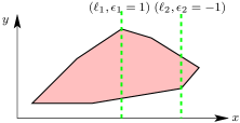
Figure 4.2: A weighted polygon of complexity $2$.

For any $s\in{\mathbb{N}}$, let

$$G_{s}:=\{-1,\,+1\}^{s}$$ (4.5)

and let

$$\mathcal{G}:=\{T^{k}\,\,|\,\,k\in{\mathbb{Z}}\},$$ (4.6)

where $T$ is the $2$ by $2$ matrix (4.3). Consider the action of the product group $G_{s}\times\mathcal{G}$ on the space $\mathcal{W}\!\!\mathop{\rm~{}Polyg}\nolimits_{s}({\mathbb{R}}^{2})$: the product

$$((\epsilon^{\prime}_{j})_{j=1}^{s},\,T^{k})\cdot\Big{(}\Delta,\,(\ell_{\lambda_{j}})_{j=1}^{s},\,(\epsilon_{j})_{j=1}^{s}\Big{)}$$

is defined to be

$$\Big{(}\!\!\mathop{\rm~{}t}\nolimits_{\vec{u}}(T^{k}(\Delta)),\,(\ell_{\lambda_{j}})_{j=1}^{s},\,(\epsilon^{\prime}_{j}\,\epsilon_{j})_{j=1}^{s}\Big{)},$$ (4.7)

where $\vec{u}=((\epsilon_{i}-\epsilon^{\prime}_{i})/2)_{i=1}^{s}$, and $\!\!\mathop{\rm~{}t}\nolimits_{\vec{u}}$ is a map of the form (4.4).

Definition 4.4   Let $\Delta$ be a rational convex polygon obtained from the momentum image $(J,\,H)(M)$ according to the proof of Theorem 4.1 by cutting along the vertical half-lines $\ell_{1}^{\epsilon_{1}},\ldots,\ell_{m_{f}}^{\epsilon_{m_{f}}}$. The semitoric polygon invariant of $(M,\,\omega,\,(J,\,H))$ is the $(G_{m_{f}}\times\mathcal{G})$-orbit

$$(G_{m_{f}}\times\mathcal{G})\cdot\Big{(}\Delta,\,(\ell_{j})_{j=1}^{m_{f}},\,(\epsilon_{j})_{j=1}^{m_{f}}\Big{)}\in\mathcal{W}\!\!\mathop{\rm~{}Polyg}\nolimits_{m_{f}}({\mathbb{R}}^{2})/(G_{m_{f}}\times\mathcal{G}),$$ (4.8)

where $\mathcal{W}\!\!\mathop{\rm~{}Polyg}\nolimits_{m_{f}}({\mathbb{R}}^{2})$ is as in Definition 4.3 and the action of $G_{m_{f}}\times\mathcal{G}$ on $\mathcal{W}\!\!\mathop{\rm~{}Polyg}\nolimits_{m_{f}}({\mathbb{R}}^{2})$ is given by (4.7). $\oslash$

It follows now from Theorem 4.1 that the semitoric polygon invariant does not depend on the isomorphism class of the system.

Lemma 4.5.

Let $(M_{1},\,\omega_{1},(J_{1},\,H_{1})),\,(M_{2},\,\omega_{2},(J_{2},\,H_{2}))$ be isomorphic $4$-dimensional semitoric integrable systems. Then the semitoric polygon invariant of $(M_{1},\,\omega_{1},(J_{1},\,H_{1}))$ is equal to the semitoric polygon invariant of $(M_{2},\,\omega_{2},(J_{2},\,H_{2}))$.

5 Geometric invariants of a semitoric system

The invariants we have described so far are not enough to determine whether two $4$-dimensional semitoric systems are isomorphic. In this section we introduce two global geometric invariants, which encode a mixture of information about local and global behavior. Throughout, $(M,\,\omega,\,(J,\,H))$ is a $4$-dimensional semitoric integrable system with $m_{f}$ isolated focus-focus singular values.

5.1 The Volume Invariant

The invariant we introduce next is easy to define using the combinatorial ingredients we have by now introduced. Consider a focus-focus critical point $m_{i}$ whose image by $(J,\,H)$ is $c_{i}$ for $i\in\{1,\,\ldots,\,m_{f}\}$, and let $\Delta$ be a rational convex polygon corresponding to the system $(M,\,\omega,\,(J,\,H))$, c.f. Definition 4.2.

Lemma 5.1.

If $\mu$ is a toric momentum map for the semitoric system $(M,\,\omega,\,(J,\,H))$ corresponding to $\Delta$, c.f. Definition 4.1, then the image $\mu(m_{i})$, where $i\in\{1,\,\ldots,\,m_{f}\}$, is a point lying in the interior of the polygon $\Delta$, along the line $\ell_{i}$. The vertical distance

$$h_{i}:=\mu(m_{i})-\min_{s\in\ell_{i}\cap\Delta}\pi_{2}(s)>0$$ (5.1)

between $\mu(m_{i})$ and the point of intersection of $\ell_{i}$ with the image polytope with lowest $y$-coordinate, is independent of the choice of momentum map $\mu$. Here $\pi_{2}\colon{\mathbb{R}}^{2}\to{\mathbb{R}}$ is the canonical projection $\pi_{2}(x,\,y)=y$.

Lemma 5.1 follows from the fact that two different toric momentum maps only differ by piecewise affine transformations, which all act on any fixed vertical line as translations.

Definition 5.2   We say that the vertical distance (5.1) bewteen $\mu(m_{i})$ and the point of intersection of $\ell_{i}$ with the image polytope that has the lowest $y$-coordinate is the height of the focus-focus critical value $c_{i}$, where $i\in\{1,\,\ldots,\,m_{f}\}$. $\oslash$

Remark 5.2   One can give a geometrical meaning to the height of the focus-focus critical values. Let $Y_{i}=J^{-1}(c_{i})$. This singular manifold splits into two parts, $Y^{+}_{i}$ and $Y^{-}_{i}$ defined as $Y_{i}\cap\{H>H(m_{i})\}$ and $Y_{i}\cap\{H<H(m_{i})\}$, respectively. The height of the focus-focus critical value $c_{i}$ is simply the Liouville volume of $Y^{-}_{i}$. $\oslash$

Since isomorphic systems share the same set of momentum polygons, we have the following result.

Lemma 5.3.

Let $(M_{1},\,\omega_{1},(J_{1},\,H_{1})),\,(M_{2},\,\omega_{2},(J_{2},\,H_{2}))$ be isomorphic $4$-dimensional semitoric integrable systems and let $(h^{j}_{i})_{i=1}^{m^{i}_{f}}$ be the tuple of heights of focus-focus critical values of of $(M_{j},\,\omega_{j},(J_{j},\,H_{j}))$, $j\in\{1,\,2\}$. Then the tuple $(h^{1}_{i})_{i=1}^{m^{1}_{f}}$ is equal to the tuple $(h^{2}_{i})_{i=1}^{m^{2}_{f}}$.

The volume invariant is very easy to compute from a weighted polygon, and hence it is a quick way to rule out that two semitoric integrable systems are not isomorphic.

5.2 The Twisting-Index Invariant

For clarity, we divide the construction of the twisting index invariant into five steps. Let

$$\Delta_{\!\!\mathop{\mbox{\rm\scriptsize~{}weight}}\nolimits}:=\Big{(}\Delta,\,(\ell_{j})_{j=1}^{m_{f}},\,(\epsilon_{j})_{j=1}^{m_{f}}\Big{)}\in\mathcal{W}\!\!\mathop{\rm~{}Polyg}\nolimits_{m_{f}}({\mathbb{R}}^{2}),$$ (5.2)

be a weighted polygon as in expression (4.8), representing the orbit given by the semitoric polygon invariant of the system $(M,\,\omega,\,(J,\,H))$, c.f. Definition 4.2, where recall that the polygon $\Delta$ is obtained from the momentum image $(J,\,H)(M)$ according to the proof of Theorem 4.1 by cutting along the vertical lines $\ell_{1},\ldots,\ell_{m_{f}}$ in the direction of $\epsilon_{1},\ldots,\epsilon_{m_{f}}$, i.e. upwards if $\epsilon_{i}$ is $+1$ and downwards otherwise. Write $F=(J,\,H)$, $c_{1},\ldots,c_{m_{f}}$ for the focus-focus critical values.

In the first three steps we define for each $i\in\{1,\,\dots,\,m_{f}\}$, an integer $k_{i}$ that we shall call the twisting index of the focus-focus value $c_{i}$, on which we built to construct the actual invariant associated to $(M,\,\omega,\,(J,\,H))$ in Step 5.

Step 1: an application of Eliasson’s theorem. Let $(e_{1},\,e_{2})$ be the canonical basis of ${\mathbb{R}}^{2}$. Let $\ell=\ell_{i}^{+1}\subset{\mathbb{R}}^{2}$ be the vertical half-line starting at $c_{i}$ and pointing in the direction of $\epsilon_{i}\,e_{2}$.

Let us apply Eliasson’s theorem in a small neighbourhood $W=W_{i}$ of the focus-focus critical point $m_{i}=F^{-1}(c_{i})$ : there exists a local symplectomorphism $\phi:({\mathbb{R}}^{4},\,0)\to W$, and a local diffeomorphism $g$ of $({\mathbb{R}}^{2},\,0)$ such that

$$F\circ\phi=g\circ q,$$ (5.3)

where $q$ is the quadratic momentum map given by (3.1). Since the second component, $q_{2}\circ\phi^{-1}$ has a $2\pi$-periodic Hamiltonian flow, it must be equal to $J$ in $W$, up to a sign. Composing if necessary $\phi$ by the canonical transformation $(x,\xi)\mapsto(-x,-\xi)$, one can always assume that $q_{2}=J\circ\phi$ in $W$. This means that $g$ is of the form

$$g(q_{1},\,q_{2})=(q_{2},\,g_{2}(q_{1},\,q_{2})).$$ (5.4)

Moreover, upon composing $\phi$ by the canonical transformation $(x,\,y,\,\xi,\,\eta)\mapsto(-\xi,\,-\eta,\,x,\,y)$, which changes $(q_{1},\,q_{2})$ into $(-q_{1},\,q_{2})$, one can always assume that

$$\frac{\partial g_{2}}{\partial q_{1}}(0)>0.$$ (5.5)

In particular, near the origin $\ell$ is transformed by $g^{-1}$ into the positive real axis if $\epsilon_{i}=1$, or the negative real axis if $\epsilon_{i}=-1$.

Step 2: the smooth vector field $\mathcal{X}_{p}$. Let us now fix the origin of angular polar coordinates in ${\mathbb{R}}^{2}$ on the positive real axis. Let $V=F(W)$ and define $\tilde{F}=(H_{1},\,H_{2})=g^{-1}\circ F$ on $F^{-1}(V)$ (notice that $H_{2}=J$). Now recall from Section 3.2 that near any regular torus there exists a Hamiltonian vector field $\mathcal{X}_{p}$, whose flow is $2\pi$-periodic, defined by

$$2\pi\mathcal{X}_{p}=(\tau_{1}\circ\tilde{F})\mathcal{X}_{H_{1}}+(\tau_{2}\circ\tilde{F})\mathcal{X}_{J},$$ (5.6)

where $\tau_{1}$ and $\tau_{2}$ are functions on ${\mathbb{R}}^{2}\setminus\{0\}$ satisfying (3.2), with $\sigma_{1}(0)>0$. In fact $\tau_{2}$ is multivalued, but we determine it completely in polar coordinates with angle in $[0,\,2\pi)$ by requiring continuity in the angle variable and $\sigma_{2}(0)\in[0,\,2\pi)$. In case $\epsilon_{i}=1$, this defines $\mathcal{X}_{p}$ as a smooth vector field on $F^{-1}(V\setminus\ell)$. In case $\epsilon_{i}=-1$ we keep the same $\tau_{2}$-value on the negative real axis, but extend it by continuity in the angular interval $[\pi,\,3\pi)$. In this way $\mathcal{X}_{p}$ is again a smooth vector field on $F^{-1}(V\setminus\ell)$.

Step 3: twisting index of a weighted polygon at a focus-focus singularity. Let $\mu$ be the generalized toric momentum map, c.f. Definition 4.1, associated to the polygon $\Delta$. On $F^{-1}(V\setminus\ell$), $\mu$ is smooth, and its components $(\mu_{1},\,\mu_{2})=(J,\,\mu_{2})$ are smooth Hamiltonians, whose vector fields $(\mathcal{X}_{J},\mathcal{X}_{\mu_{2}})$ are tangent to the foliation, have a $2\pi$-periodic flow, and are a.e. independent. Since the couple $(\mathcal{X}_{J},\mathcal{X}_{p})$ shares the same properties, there must be a matrix $A\in\textup{GL}(2,{\mathbb{Z}})$ such that $(\mathcal{X}_{J},\mathcal{X}_{\mu_{2}})=A(\mathcal{X}_{J},\mathcal{X}_{p})$. This is equivalent to saying that there exists an integer $k_{i}\in{\mathbb{Z}}$ such that

$$\mathcal{X}_{\mu_{2}}=k_{i}\mathcal{X}_{J}+\mathcal{X}_{p}.$$ (5.7)

Proposition 5.4.

For a fixed weighted polygon $\Delta_{\!\!\mathop{\mbox{\rm\scriptsize~{}weight}}\nolimits}$ as in equation (5.2), the integer $k_{i}$ in (5.7) is well defined for each $i\in\{1,\,\ldots,\,m_{f}\}$, i.e. it does not depend on

• the choice of the periodic Hamiltonian $\mathcal{X}_{p}$;

• the transformations involved in Eliasson’s normal form (5.3), with the sign constraints (5.4) and (5.5).

Proof.

It follows from Lemma 4.1 in [21] that changing the transformations involved in Eliasson’s normal form [7] can only modify $g_{2}$ — and hence $H_{1}$ — by a flat term. Suppose $\mathcal{X}_{p}^{\prime}$ is another admissible choice for a Hamiltonian of the form

$$2\pi\mathcal{X}_{p}^{\prime}=(\tau_{1}^{\prime}\circ\tilde{F}^{\prime})\mathcal{X}_{H_{1}^{\prime}}+(\tau_{2}^{\prime}\circ\tilde{F}^{\prime})\mathcal{X}_{J}.$$

Since $\mathcal{X}_{p}^{\prime}$ has a $2\pi$-periodic flow, there must be coprime integers $a,\,b$ in ${\mathbb{Z}}$ such that

$$\mathcal{X}_{p}^{\prime}=a\mathcal{X}_{p}+b\mathcal{X}_{J}.$$ (5.8)

Inserting (5.6), we see that there exist functions $Z_{1}$ and $Z_{2}$ that vanish at all orders at the origin such that

$$2\pi\mathcal{X}_{p}^{\prime}=(a\tau_{1}\circ\tilde{F}+Z_{1})\mathcal{X}_{H_{1}^{\prime}}+(a\tau_{2}\circ\tilde{F}+2\pi b+Z_{2})\mathcal{X}_{J}.$$

From this we see that, up to a flat function, $\tau_{1}^{\prime}=a\tau_{1}$ and $\tau_{2}^{\prime}=a\tau_{2}+2\pi b$. Because of the logarithmic asymptotics required in (3.2), the first equation requires $a=1$. But then, the second equation with the restriction that both $\sigma_{2}(0)$ and $\sigma_{2}^{\prime}(0)$ must be in $[0,2\pi)$ implies that $b=0$. Recalling (5.8) we obtain $\mathcal{X}_{p}^{\prime}=\mathcal{X}_{p}$, which shows that $k_{i}$ is indeed well-defined. ∎

Definition 5.5   Let $\Delta_{\!\!\mathop{\mbox{\rm\scriptsize~{}weight}}\nolimits}$ be a fixed weighted polygon as in (5.2). For each $i\in\{1,\,\ldots,\,m_{f}\}$, the integer $k_{i}$ defined in equation (5.7) is called the twisting index of $\Delta_{\!\!\mathop{\mbox{\rm\scriptsize~{}weight}}\nolimits}$ at the focus-focus critical value $c_{i}$. $\oslash$

The integer $k_{i}$ in Definition 5.4 is still not the relevant object that we intend to associate to the semitoric system, but we shall build on its definition to construct the actual invariant.

Step 4: the privileged momentum map. We explain how there is a reasonable way to “choose” a momentum map for $(M,\,\omega,\,(J,\,H))$.

Lemma 5.6.

There exists a unique smooth function $H_{p}$ on $F^{-1}(V\setminus\ell)$ the Hamiltonian vector field of which is $\mathcal{X}_{p}$ and such that $\lim_{m\to m_{i}}H_{p}=0.$

Proof.

Near a regular torus $\mathcal{X}_{p}$ is a Hamiltonian vector field of a function of the form $f(H_{1},\,J)$, and by construction $\partial_{i}f=\tau_{i}/2\pi,$ $i\in\{1,\,2\}$. Therefore, using (3.2) we can check that $2\pi f(z)=S(c)-\Re(z\ln z-z)+\textup{Const},$ where $S$ is smooth at the origin, which shows that $f$ has a limit as $z\in{\mathbb{R}}^{2}\setminus([0,\,\infty)\times\{0\})$ tends to the origin. In fact, $f$ has a continuous extension to ${\mathbb{R}}^{2}$, entailing that $H_{p}$ extends to a continuous function on $F^{-1}(V)$. ∎

Definition 5.7   Let $(M,\,\omega,\,(J,\,H))$ be a $4$-dimensional semitoric integrable system, and let $H_{p}$ be the unique smooth function defined in Lemma 5.6. We say that the toric momentum map $\nu:=(J,\,H_{p})$ is the privileged momentum map for $(J,\,H)$ around the focus-focus value $c_{i}$, for each $i\in\{1,\,\ldots,\,m_{f}\}$. $\oslash$

Remark 5.7   The map $\nu$ in Definition 5.6 depends on the cut $\ell$, that is to say, on the sign $\epsilon_{i}$. Moreover, we have the following.

• If $k_{i}$ is the twisting index of $c_{i}$, one has

  $$\mu=T^{k_{i}}\nu\qquad\text{ on }F^{-1}(V).$$ (5.9)

• If we transform the polygon $\Delta$ by a global affine transformation in $T^{r}\in\mathfrak{I}$ this has no effect on the privileged momentum map $\nu$, whereas it changes $\mu$ into $T^{r}\mu$.

From the characterization (5.9), it follows that all the twisting indices $k_{i}$ are replaced by $k_{i}+r$. $\oslash$

With this preparation we are now ready to define the twisting index invariant.

Step 5: the twisting index invariant. We give the definition of the twisting index invariant as an equivalence class of weighted polygons pondered by a collection of integers.

Proposition 5.8.

If two weighted polygons $\Delta_{\!\!\mathop{\mbox{\rm\scriptsize~{}weight}}\nolimits}$ and $\Delta^{\prime}_{\!\!\mathop{\mbox{\rm\scriptsize~{}weight}}\nolimits}$ lie in the same $G_{m_{f}}$-orbit, for the $G_{m_{f}}$-action induced by (4.7), then the twisting indexes $k_{i},\,k^{\prime}_{i}$ associated to $\Delta_{\!\!\mathop{\mbox{\rm\scriptsize~{}weight}}\nolimits}$ and $\Delta^{\prime}_{\!\!\mathop{\mbox{\rm\scriptsize~{}weight}}\nolimits}$ at their respective focus-focus critical values $c_{i},\,c^{\prime}_{i}$ are equal, for each $i\in\{1,\,\ldots,\,m_{f}\}$.

Proof.

For $\epsilon_{i}=\pm 1$, we denote by $\mu_{\pm}$ and $\nu_{\pm}$, as in equation (5.9) above, the generalized toric momentum map and the privileged momentum map, c.f. Definition 5.6 at $c_{i}$.

With the notations of Section 4, we have

$$\mu_{-}=\!\!\mathop{\rm~{}t}\nolimits_{\ell_{i}}\mu_{+}.$$

On the other hand, from the definition of $\tau_{2}$ in each case, we see that $\mathcal{X}_{p,-}=\mathcal{X}_{p,+}$ on the left-hand side of $\ell$ (that is to say, $J<0$), while

$$\mathcal{X}_{p,-}=\mathcal{X}_{p,+}+2\pi\mathcal{X}_{J}$$

on the right hand side ($J>0$). This means that $\nu_{-}=\!\!\mathop{\rm~{}t}\nolimits_{\ell_{i}}\nu_{+}$. From the characterization of the twisting index by (5.9), using that $\!\!\mathop{\rm~{}t}\nolimits_{\ell_{i}}$ commutes with $T$, we see that $k_{i,+}=k_{i,-}$. ∎

Recall the groups $G_{s}$ and $\mathcal{G}$ given by (4.5) and (4.6) respectively, and the action of $G_{s}\times\mathcal{G}$ on $\mathcal{W}\!\!\mathop{\rm~{}Polyg}\nolimits_{s}({\mathbb{R}}^{2})$, c.f. Definition 4.7. Consider the action of the product group $G_{s}\times\mathcal{G}$ on the space $\mathcal{W}\!\!\mathop{\rm~{}Polyg}\nolimits_{s}({\mathbb{R}}^{2})\times{\mathbb{Z}}^{m_{s}}$: the product

$$((\epsilon^{\prime}_{j})_{j=1}^{s}),\,T^{k})\star\Big{(}\Delta,\,(\ell_{\lambda_{j}})_{j=1}^{s},\,(\epsilon_{j})_{j=1}^{s},\,(k_{i})_{i=1}^{s}\Big{)}$$

is defined to be

$$\Big{(}\!\!\mathop{\rm~{}t}\nolimits_{\vec{u}}(T^{k}(\Delta)),\,(\ell_{\lambda_{j}})_{j=1}^{s},\,(\epsilon^{\prime}_{j}\,\epsilon_{j})_{j=1}^{s},\,(k_{i}+k)_{i=1}^{s}\Big{)}.$$ (5.10)

where $\vec{u}=(\epsilon_{i}-\epsilon^{\prime}_{i})/2)_{i=1}^{s}$. Here $T$ is the $2$ by $2$ matrix (4.3) and $\!\!\mathop{\rm~{}t}\nolimits_{\vec{u}}$ is of the form (4.4).

Definition 5.9   The twisting-index invariant of $(M,\,\omega,\,(J,\,H))$ is the $(G_{m_{f}}\times\mathcal{G})$-orbit of weighted polygon pondered by twisting indexes at the focus-focus singularities of the system given by

$$(G_{m_{f}}\times\mathcal{G})\star\Big{(}\Delta,\,(\ell_{j})_{j=1}^{m_{f}},\,(\epsilon_{j})_{j=1}^{m_{f}},\,(k_{i})_{i=1}^{m_{f}}\Big{)}\in(\mathcal{W}\!\!\mathop{\rm~{}Polyg}\nolimits_{m_{f}}({\mathbb{R}}^{2})\times{\mathbb{Z}}^{m_{f}})/(G_{m_{f}}\times\mathcal{G}),$$ (5.11)

where $\mathcal{W}\!\!\mathop{\rm~{}Polyg}\nolimits_{m_{f}}({\mathbb{R}}^{2})$ is defined in Definition 4.3 and the action of $G_{m_{f}}\times\mathcal{G}$ on $\mathcal{W}\!\!\mathop{\rm~{}Polyg}\nolimits_{m_{f}}({\mathbb{R}}^{2})\times{\mathbb{Z}}^{m_{f}}$ is given by (5.10). $\oslash$

Here again, our definition is invariant under isomorphism.

Lemma 5.10.

Let $(M_{1},\,\omega_{1},(J_{1},\,H_{1})),\,(M_{2},\,\omega_{2},(J_{2},\,H_{2}))$ be isomorphic $4$-dimensional semitoric integrable systems. Then their corresponding twisting-index invariants are equal.

Remark 5.10   We would like to emphasize again that the twisting index is not a semiglobal invariant of the singular fibration in a neighbourhood of the focus-focus fibre. Such semiglobal fibrations are completely classified in [21], and the twisting index does not play any role there. It is instead a global invariant characterizing the way the fibers near a particular focus-focus point stand with respect to the rest of the fibration. $\oslash$

6 Main Theorem: Statement

To each semitoric system we assign a list of invariants as above.

Definition 6.1   Let $(M,\,\omega,\,(J,\,H))$ be a $4$-dimensional semitoric integrable system. The list of invariants of $(M,\,\omega,\,(J,\,H))$ consists of the following items.

• The integer number $0\leq m_{f}<\infty$ of focus-focus singular points, see Section 3.1.

• The $m_{f}$-tuple $((S_{i})^{\infty})_{i=1}^{m_{f}}$, where $(S_{i})^{\infty}$ is the Taylor series of the $i^{\!\!\mathop{\mbox{\rm\scriptsize~{}th}}\nolimits}$ focus-focus point, see Section 3.2.

• The semitoric polygon invariant: the $(G_{m_{f}}\times\mathcal{G})$-orbit

  $$(G_{m_{f}}\times\mathcal{G})\cdot\Delta_{\!\!\mathop{\mbox{\rm\scriptsize~{}weight}}\nolimits}\,\,\in\,\,\mathcal{W}\!\!\mathop{\rm~{}Polyg}\nolimits({\mathbb{R}}^{2})/(G_{m_{f}}\times\mathcal{G})$$

  of the weighted polygon $\Delta_{\!\!\mathop{\mbox{\rm\scriptsize~{}weight}}\nolimits}:=\Big{(}\Delta,\,(\ell_{j})_{j=1}^{m_{f}},\,(\epsilon_{j})_{j=1}^{m_{f}}\Big{)}$, c.f. Definition 4.2.

• The $m_{f}$-tuple of integers $(h_{i})_{i=1}^{m_{f}}$, where $h_{i}$ is the height of the $i^{\!\!\mathop{\mbox{\rm\scriptsize~{}th}}\nolimits}$ focus-focus point, see Section 5.1.

• The twisting-index invariant: the $(G_{m_{f}}\times\mathcal{G})$-orbit

  $$(G_{m_{f}}\times\mathcal{G})\star\Big{(}\Delta_{\!\!\mathop{\mbox{\rm\scriptsize~{}weight}}\nolimits},\,(k_{i})_{i=1}^{m_{f}}\Big{)}\,\,\in\,\,(\mathcal{W}\!\!\mathop{\rm~{}Polyg}\nolimits({\mathbb{R}}^{2})\times{\mathbb{Z}}^{m_{f}})/(G_{m_{f}}\times\mathcal{G})$$

  of the weighted polygon pondered by the twisting-indexes $\Big{(}\Delta_{\!\!\mathop{\mbox{\rm\scriptsize~{}weight}}\nolimits},\,(k_{i})_{i=1}^{m_{f}}\Big{)}$, c.f. Definition 5.8.

$\oslash$

In the above list invariant (v) determines invariant (iii), so we could have ignored the latter. We have kept this list as it appears naturally in the construction of the invariants. Indeed the definition of invariant (iii) is needed to construct invariant (v). One may also argue that it is worthwhile for practical purposes to list (iii), as it is easier to compute than (v) and hence if two systems do not have the same invariant (iii) we know they are not isomorphic without having to compute (v).

Recall that if $(M_{1},\,\omega_{1},\,(J_{1},\,H_{1}))$ and $(M_{2},\,\omega_{2},\,(J_{2},\,H_{2}))$ are $4$-dimensional semitoric integrable systems, we say that they are isomorphic if there exists a symplectomorphism

$$\varphi\colon M_{1}\to M_{2},\,\,\,\,\,\,\,\textup{such that}\,\,\,\,\,\varphi^{*}(J_{2},\,H_{2})=(J_{1},\,f(J_{1},\,H_{1})).$$

for some smooth function $f$. Our main theorem is the following.

Theorem 6.2.

Two $4$-dimensional semitoric integrable systems $(M_{1},\,\omega_{1},(J_{1},\,H_{1})),\,(M_{2},\,\omega_{2},(J_{2},\,H_{2}))$ are isomorphic if and only if the list of invariants (i)-(v), as in Definition 6, of $(M_{1},\,\omega_{1},(J_{1},\,H_{1}))$ is equal to the list of invariants (i)-(v) of $(M_{2},\,\omega_{2},(J_{2},\,H_{2}))$.

The proof of Theorem 6.2 is sufficiently involved that is better organized in an independent section. In the proof we combine notable results of several authors, in particular Eliasson, Duistermaat, Dufour-Molino, Liouville-Mineur-Arnold and Vũ Ngọc. We combine these results with new ideas to construct explicitly an isomorphism between two semitoric integrable systems that have the same invariants, in the spirit of Delzant’s proof [3] for the case when the system defines a Hamiltonian $2$-torus action. Because in our context we have focus-focus singularities a number of delicate problems arise that one has to deal with to construct such an isomorphism. As a matter of fact, it is remarkable how the behavior of the system near a particular singularity has a subtle global effect on the system.

7 Proof of Main Theorem

The left-to-right implication follows from putting together lemmas 3.2, 3.4, 4.5, 5.3 and 5.10. The proof of the right-to-left implication breaks into three steps. Let $F_{1}=(J_{1},\,H_{1})$ and let $F_{2}=(J_{2},\,H_{2})$.

• First, we reduce to a case where the images $F_{1}(M_{1})$ and $F_{2}(M_{2})$ are equal.

• Second, we prove that this common image can be covered by open sets $\Omega_{\alpha}$, above each of which $F_{1}$ and $F_{2}$ are symplectically interwined.

• The last step is to glue together these local symplectomorphisms, in this way constructing a global symplectomorphism $\phi:M_{1}\to M_{2}$ such that $F_{1}=F_{2}\circ\phi$.

Step 1: first reduction. The goal of this step is to reduce to a particular case where the images $F_{1}(M_{1})$ and $F_{2}(M_{2})$ are equal. For simplicity we assume that the invariants of $F_{1}$ are indexed as in Definition 6 with an additional upper index $1$, and similarly for $F_{2}$.

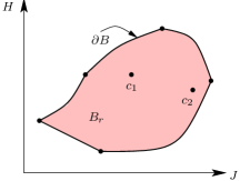
Figure 7.1: In Step 1 we prove that we can assume that the “momentum” images $F_{1}(M_{1})$ and $F_{2}(M_{2})$ are equal to the same curved polygon $B$. To emphasize this we index the axes as $J$ and $H$ without lower indexes.

Because both systems have the same invariants (i), (iii) and (v), we may choose a weighted polygon pondered by the twisting indexes $\Big{(}\Delta_{\!\!\mathop{\mbox{\rm\scriptsize~{}weight}}\nolimits},\,(k_{i})_{i=1}^{m_{f}}\Big{)},$ where $\Delta_{\!\!\mathop{\mbox{\rm\scriptsize~{}weight}}\nolimits}=\Big{(}\Delta,\,(\ell_{j})_{j=1}^{m_{f}},\,(\epsilon_{j})_{j=1}^{m_{f}}\Big{)},$ and which is inside of the $(\mathcal{W}\!\!\mathop{\rm~{}Polyg}\nolimits({\mathbb{R}}^{2})\times{\mathbb{Z}}^{m^{1}_{f}})/(G_{m^{1}_{f}}\times\mathcal{G})=(\mathcal{W}\!\!\mathop{\rm~{}Polyg}\nolimits({\mathbb{R}}^{2})\times{\mathbb{Z}}^{m_{f}^{2}})/(G_{m^{2}_{f}}\times\mathcal{G})$-orbit of weighted polygons pondered by twisting indexes:

$$(G_{m^{1}_{f}}\times\mathcal{G})\star\Big{(}\Delta^{1}_{\!\!\mathop{\mbox{\rm\scriptsize~{}weight}}\nolimits}\,(k^{1}_{i})_{i=1}^{m^{1}_{f}}\Big{)}=(G_{m^{2}_{f}}\times\mathcal{G})\star\Big{(}\Delta^{2}_{\!\!\mathop{\mbox{\rm\scriptsize~{}weight}}\nolimits},\,(k^{2}_{i})_{i=1}^{m^{2}_{f}}\Big{)},$$ (7.1)

where we are writing $\Delta^{i}_{\!\!\mathop{\mbox{\rm\scriptsize~{}weight}}\nolimits}=(\Delta^{i},\,(\ell^{i}_{j})_{j=1}^{m^{i}_{f}},\,(\epsilon^{i}_{j})_{j=1}^{m^{i}_{f}}\Big{)}$, for $i\in\{1,\,2\}$.

Let $\mu_{1},\,\mu_{2}$ respectively be associated toric momentum maps to $F_{1}$ and $F_{2}$ for the polygon $\Delta$ in Theorem 4.1 and Definition 4.1. There are homeomorphisms $g_{1},\,g_{2}\colon\Delta\to\Delta$ such that

$$F_{1}=g_{1}\circ\mu_{1},\,\,\,\,F_{2}=g_{2}\circ\mu_{2}.$$

Consider the map $h:=g_{1}\circ g_{2}^{-1}$. We wish to replace $F_{2}$ by $\widetilde{F}_{2}=h\circ F_{2}$. Then, obviously,

$$\!\!\mathop{\rm~{}Image}\nolimits(\widetilde{F}_{2})=g_{1}(\Delta)=\!\!\mathop{\rm~{}Image}\nolimits({F}_{1}).$$

In order for $\widetilde{F}_{2}$ to define a semi-toric completely integrable system isomorphic to $F_{2}$, we need to prove that $h(x,\,y)=(x,\,f(x,y))$ for some smooth function $f$. In fact, it follows from Theorem 4.1 that $h$ has this form, but for some $f$ which is a priori not smooth. The crucial point here is to show that, because $F_{1}$ and $F_{2}$ have the same invariants, $h$ is in fact smooth.

Claim 7.1.

The map $h$ extends to an $S^{1}$-equivariant diffeomorphism of a neighborhood of $F_{2}(M_{2})$ into a neighborhood of $F_{1}(M_{1})$.

The map $h$ is a already a homeomorphism. We need to show that it is a local diffeomorphism everywhere. Let us denote by $c_{i}^{j}$ for $j\in\{1,\,2\}$ and $i\in\{1,\,\dots,\,m_{f}\}$ the focus-focus critical values of $F_{j}$. Again we let $(e_{1},\,e_{2})$ be the canonical basis of ${\mathbb{R}}^{2}$ and let $\ell_{i}^{j}\subset{\mathbb{R}}^{2}$ be the vertical half-line starting at $c_{i}^{j}$ and pointing in the direction of $\epsilon_{j}e_{2}$.

Since the tuple of heights of the focus-focus points given by invariant (iv) are the same for both systems, $g_{1}^{-1}(c_{j}^{1})=g_{2}^{-1}(c_{j}^{2})$ and $g_{1}^{-1}(\ell_{i}^{1})=g_{2}^{-1}(\ell_{i}^{2})$. Hence $h$ is smooth away from the union of all $\ell_{i}^{2}$, $i\in\{1,\,\dots,\,m_{f}\}$.

Let us now fix some $i\in\{1,\dots,m_{f}\}$ and let $\widetilde{U}_{z}$ be a small ball around a point $z\in\ell_{i}^{2}\setminus\{c_{i}^{2}\}$. For simplifying notations, we shall drop the various subscripts $i$. Recall that $\widetilde{U}_{z}$ inherits from $F_{2}(M_{2})$ an integral-affine structure. Let $\varphi_{z}:U_{z}\to\widetilde{U}_{z}$ be an oriented affine chart, with $U_{z}$ a neighborhood of the origin in ${\mathbb{R}}^{2}$, sending the vertical axis to $\ell^{2}$. In order to show that $h$ is smooth on $\widetilde{U}_{z}$, we consider the two halves of the ball $\widetilde{U}_{z}$ :

$$\widetilde{U}_{z}^{+}=\widetilde{U}_{z}\cap\{x\geq x_{c}\}\,\,\,\textup{ and}\,\,\,\widetilde{U}_{z}^{-}=\widetilde{U}_{z}\cap\{x\leq x_{c}\},$$

where $x_{c}$ is the abscissa of $c^{2}$. Of course, the restrictions of $\varphi_{z}$ to each half $U_{z}\cap\{x\geq 0\}$ and $U_{z}\cap\{x\leq 0\}$ are admissible affine charts for $\widetilde{U}_{z}^{+}$ and $\widetilde{U}_{z}^{-}$, respectively. Let us call these restrictions $\varphi^{\pm}_{z}$. Let $y=h(z)$, $\widetilde{V}_{y}=h(\widetilde{U}_{z})$ and $\widetilde{V}_{y}^{\pm}=h(\widetilde{U}_{z}^{\pm})$. Using the natural integral-affine structure on $F_{1}(M_{1})$, we can similarly introduce an affine chart $\psi_{y}$ for $\widetilde{V}_{y}$ and the corresponding restrictions $\psi_{y}^{\pm}$. We are now going to use the following facts :

1. On each half $\widetilde{U}_{z}^{+}$ and $\widetilde{U}_{z}^{-}$, $h$ is an integral-affine isomorphism : $\widetilde{U}_{z}^{\pm}\to\widetilde{V}_{y}^{\pm}$.

2. The differential $\!\!\mathop{\rm~{}d}\nolimits h$ is continuous on $\widetilde{U}$.

The first fact implies, by definition, that the map

$$\nu^{\pm}:=(\psi^{\pm}_{y})^{-1}\circ h\circ\varphi^{\pm}_{z},$$

wherever defined, is of the form $A^{\pm}(\cdot)+b^{\pm},$ for some matrix $A^{\pm}\in\textup{GL}(2,\,\mathbb{Z})$ and some constant $b^{\pm}\in\mathbb{R}^{2}$. Evaluating the differentials at the origin, we immediately deduce from the second fact that $A^{+}=A^{-}$. So, $\nu^{\pm}$ should be just a translation. But $h$ itself being continuous on the line segment $\ell^{2}$, we must have $b^{+}=b^{-}$. It follows that, on $\widetilde{U}_{z}$, $h$ is equal to $\psi_{y}\circ L\circ\varphi_{z}^{-1}$, where $L$ is the affine transformation $A^{+}(\cdot)+b^{+}=A^{-}(\cdot)+b^{-}$. So $h$ is indeed smooth on $\widetilde{U}_{z}$.

We have left to show that $h$ is smooth at a focus-focus critical value $c^{2}$. The fact that we are assuming that invariant (ii) is the same for both systems means that the corresponding symplectic invariants power series $(S)^{\infty}$ are the same for both systems implies, by the semi-global result of Vũ Ngọc [21, Th. 2.1], that there exist a neighborhood $V(c^{1})$ of $c^{1}$, a neighborhood $V(c^{2})$ of $c^{2}$, a semi-global symplectomorphism $\varphi:F_{1}^{-1}(V(c^{1})))\to F_{2}^{-1}(V(c^{2}))$ and a local diffeomorphism $g:V(c^{2})\to V(c^{1})$ such that $F_{1}=g\circ F_{2}\circ\varphi$. Now, from Lemma 5.6 we know that there exists a privileged toric momentum map, c.f. Definition 5.6, for each system above the domain $V(c^{j})\setminus\ell^{j}$, $j\in\{1,\,2\}$, c.f. Definition 5.6. We denote by $\nu_{1}$ this momentum map for the system induced by $F_{1}$, and $\nu_{2}$ for the system induced by $F_{2}$. Since $\nu_{1}$ and $\nu_{2}$ are semi-global symplectic invariants, one has $\nu_{1}=\nu_{2}\circ\varphi$.

By equation (7.1) the focus-focus critical values $c^{1}$ of the semitoric systems $F_{1}$ and and $c^{2}$ of $F_{2}$ have the same twisting-index invariant $k$ with respect to the common polygon $\Delta$. In view of the characterization of expresion (5.9), we get

$$\mu_{1}=T^{k}\nu_{1}\qquad\text{ and }\qquad\mu_{2}=T^{k}\nu_{2},$$ (7.2)

and therefore

$$\mu_{1}=\mu_{2}\circ\varphi.$$

Thus we can write $g_{1}^{-1}F_{1}=g_{2}^{-1}F_{2}\circ\varphi$, or

$$F_{1}=h\circ g^{-1}\circ F_{1}.$$

Using that $F_{1}$ is a submersion on a neighborhood of any regular torus, and the fact that $h\circ g^{-1}$ is smooth at the corresponding regular values of $F_{1}$, we get that

$$h\circ g^{-1}=\textup{Id}\qquad\text{ on }V(c^{1}).$$ (7.3)

By continuity, this also holds at $c^{1}$. Hence $h=g$ is smooth at $c^{2}$, which proves the claim.
 
Step 2: Local symplectomorphisms. From step 1 we can assume that

$$F_{1}=g_{1}\circ\mu_{1}\quad F_{2}=g_{1}\circ\mu_{2}$$ (7.4)

and hence $F_{1}(M_{1})=F_{2}(M_{2})$. In this second step we prove that this common image can be covered by open sets $\Omega_{\alpha}$, above each of which $F_{1}$ and $F_{2}$ are symplectically interwined.

Claim 7.2.

There exists a locally finite open cover $(\Omega_{\alpha})_{\alpha\in A}$ of $F_{1}(M_{1})=F_{2}(M_{2})$ such that

1. all $\Omega_{\alpha}$, $\alpha\in A$ are simply connected, and all intersections are simply connected;

2. for each $\alpha\in A$, $\Omega_{\alpha}$ contains at most one critical value of rank $0$ of $F_{i}$, for any $i\in\{1,\,2\}$;

3. for each $\alpha\in A$, there exists a symplectomorphism $\varphi_{\alpha}:F_{1}^{-1}(\Omega_{\alpha})\to{F}_{2}^{-1}(\Omega_{\alpha})$ such that

   $$F_{1}={F}_{2}\circ\varphi_{\alpha}\quad\text{ on }F_{1}^{-1}(\Omega_{\alpha}).$$

We prove this claim next. Recall that the toric momentum maps $\mu_{1}$ and $\mu_{2}$ have by hypothesis the same image, which is the polygon $\Delta$. We can define an open cover $\tilde{\Omega}_{\alpha}$ of $\Delta$ with open balls, satisfying points $(1)$ and $(2)$. When the ball $\tilde{\Omega}_{\alpha}$ contains critical value of rank 0, we may assume that this critical value is located at its center. Similarly, when a ball contains critical values of rank 1, we may assume that the set of rank 1 critical values in this ball is a diameter. Then we just define

$$\Omega_{\alpha}=g_{1}(\tilde{\Omega}_{\alpha}).$$

Notice that in doing so we ensure that the number and type of critical values of $F_{i}$ in $\Omega_{\alpha}$ are the same for $i=1$ and $i=2$. For proving point $(3)$ we distinguish four cases :

• $\Omega_{i,\alpha}$ contains no critical point of $F_{i}$;

• $\Omega_{i,\alpha}$ contains critical points of rank 1, but not of rank 0;

• $\Omega_{i,\alpha}$ contains a rank 0 critical point, of elliptic-elliptic type;

• $\Omega_{i,\alpha}$ contains a rank 0 critical point, of focus-focus type.

The reasoning for all cases follows the same lines, but we keep these cases separated for the sake of clarity.

Case (a).

Let us fix a point $c_{\alpha}\in\Omega_{\alpha}$. By Liouville-Mineur-Arnold theorem [4], applied for each momentum map $F_{i}$ over the simply connected open set $\Omega_{\alpha}$, there exists a symplectomorphism $\tilde{\varphi}_{i,\alpha}:F_{i}^{-1}(\Omega_{\alpha})\to\!\!\mathop{\rm~{}T}\nolimits^{*}{\mathbb{T}}^{2}$ and a local diffeomorphism $h_{i}:({\mathbb{R}}^{2},\,0)\to({\mathbb{R}}^{2},\,c_{\alpha})$ such that

$$F_{i}=h_{i}(\xi_{1},\xi_{2})\circ\tilde{\varphi}_{i,\alpha}.$$

Here we use the notation $(x_{1},\,x_{2},\,\xi_{1},\,\xi_{2})$ for canonical coordinates in $\!\!\mathop{\rm~{}T}\nolimits^{*}{\mathbb{T}}^{2}$, where the zero section is given by $\{\xi_{1}=\xi_{2}=0\}$.

In fact because of equation (7.4), $\mu_{i}=g_{1}^{-1}h_{i}(\xi_{1},\,\xi_{2})\circ\tilde{\varphi}_{i,\alpha}$. Since both $\mu_{i}$ and $(\xi_{1},\,\xi_{2})$ are toric momentum map, this implies that $g_{1}^{-1}h_{i}$ is an affine map with a linear part $B_{i}\in\!\!\mathop{\rm~{}GL}\nolimits(2,\,{\mathbb{Z}})$. Now we can define a linear symplectomorphism in a block-diagonal way

$$S_{i}=\begin{pmatrix}\raisebox{2.58334pt}{${\scriptstyle t}$}B_{i}&0\\ 0&B_{i}^{-1}.\end{pmatrix}$$

Obviously $(\xi_{1},\xi_{2})\circ S_{i}=B_{i}^{-1}\circ(\xi_{1},\xi_{2})$. From now on we replace $\tilde{\varphi}_{i,\alpha}$ by $S_{i}\circ\tilde{\varphi}_{i,\alpha}$, which reduces us to the case $B_{i}=\textup{Id}$.

Now, let $\varphi_{\alpha}:=\tilde{\varphi}_{2,\alpha}^{-1}\circ\tilde{\varphi}_{1,\alpha}$. We have the relation

$$F_{1}=(h_{1}h_{2}^{-1})\circ F_{2}\circ\tilde{\varphi}_{2,\alpha}^{-1}\circ\tilde{\varphi}_{1,\alpha}=g_{1}(g_{1}^{-1}h_{1})(g_{1}^{-1}h_{2})^{-1}g_{1}^{-1}\circ\varphi_{\alpha}.$$

The affine diffeomorphism $(g_{1}^{-1}h_{1})(g_{1}^{-1}h_{2})^{-1}$ is tangent to the identity and fixes the point $c_{\alpha}$; hence it is the identity, and we obtain, as required :

$$F_{1}=F_{2}\circ\varphi_{\alpha},\quad\text{ on }F_{1}^{-1}(\Omega_{\alpha}).$$

Case (b).

Above $\Omega_{\alpha}$, the momentum map has singularities, so we cannot apply the action-angle theorem. However, there is still a ${\mathbb{T}}^{2}$-action, and it is well known that an “action-angle with elliptic singularities” theorem holds (see [6] or  [16]). Precisely, we fix a point $c_{\alpha}\in\Omega_{\alpha}$ that is a critical value of $F_{1}$ and $F_{2}$, and then for each $i\in\{1,\,2\}$, there exists a symplectomorphism $\tilde{\varphi}_{i,\alpha}:F_{i}^{-1}(\Omega_{\alpha})\to\!\!\mathop{\rm~{}T}\nolimits^{*}{\mathbb{R}}\times\!\!\mathop{\rm~{}T}\nolimits^{*}{\mathbb{T}}^{1}$ and a local, orientation preserving diffeomorphism $h_{i}:({\mathbb{R}}^{2},\,0)\to({\mathbb{R}}^{2},\,c_{\alpha})$ such that

$$F_{i}=h_{i}(q_{1},\xi_{2})\circ\tilde{\varphi}_{i,\alpha}.$$

Here $\!\!\mathop{\rm~{}T}\nolimits^{*}{\mathbb{R}}$ has canonical coordinates $(x_{1},\,\xi_{1})$, $q_{1}=(x_{1}^{2}+\xi_{1}^{2})/2$, and $\!\!\mathop{\rm~{}T}\nolimits^{*}{\mathbb{T}}^{1}$ has canonical coordinates $(x_{2},\,\xi_{2})$. As before, one has

$$\mu_{i}=g_{1}^{-1}h_{i}(q_{1},\,\xi_{2})\circ\tilde{\varphi}_{i,\alpha},$$

and $g_{1}^{-1}h_{i}$ is an affine map with a linear part in $\textup{SL}(2,{\mathbb{Z}})$.

Since $h_{i}$ must preserve the set of critical values, it must send the vertical axis “$q_{1}=0$”$\subset{\mathbb{R}}^{2}$ to the set of critical values in $\Omega_{\alpha}$. Hence $g_{1}^{-1}h_{i}$ sends the vertical axis to the corresponding diameter in $\tilde{\Omega}_{\alpha}$. Moreover, since by hypothesis the images of $\mu_{1}$ and $\mu_{2}$ are the same, the set “$q_{1}>0$” corresponds via $g_{1}^{-1}h_{1}$ and $g_{1}^{-1}h_{2}$ to the same half of the ball $\tilde{\Omega}_{\alpha}$. In other words, the vector $e_{2}=(0,1)$ is an eigenvector for the linear part $B$ of $(g_{1}^{-1}h_{1})^{-1}g_{1}^{-1}h_{2}$, with eigenvalue 1.

Therefore, $B$ is of the form $\begin{pmatrix}1&0\\ k&1\end{pmatrix}$, for some integer $k\in{\mathbb{Z}}$. Now, consider the map $S(x_{1},\,x_{2},\,\xi_{1},\,\xi_{2})=(x_{1}^{\prime},\,x_{2}^{\prime},\,\xi_{1}^{\prime},\,\xi_{2}^{\prime})$ given by

$$\left\{\begin{aligned} (x_{1}^{\prime}+i\xi_{1}^{\prime})&=\textup{e}^{ikx_{2}}(x_{1}+i\xi_{1})\\ x_{2}^{\prime}&=x_{2}\\ \xi_{2}^{\prime}&=\xi_{2}+kq_{1}.\end{aligned}\right.$$ (7.5)

In complex coordinates,

$$\!\mathop{\rm d\!}\nolimits{}\xi_{1}\wedge\!\mathop{\rm d\!}\nolimits{}x_{1}=\frac{1}{2i}\!\mathop{\rm d\!}\nolimits{}z_{1}\wedge\!\mathop{\rm d\!}\nolimits{}\bar{z}_{1},$$

so it is easy to check that $S$ is symplectic. Moreover,

$$(q_{1},\xi_{2})\circ S=\begin{pmatrix}1&0\\ k&1\end{pmatrix}(q_{1},\xi_{2})=B(q_{1},\xi_{2}).$$

We can write

$$F_{1}=h_{1}B^{-1}(q_{1},\xi_{2})\circ S\circ\tilde{\varphi}_{1,\alpha},$$

and hence, letting $\varphi_{\alpha}:=\tilde{\varphi}_{2,\alpha}^{-1}\circ S\circ\tilde{\varphi}_{\alpha}$,

$$F_{1}=(h_{1}B^{-1}h_{2}^{-1})\circ F_{2}\circ\varphi_{\alpha}.$$

Consider the affine map $(g_{1}^{-1}h_{1})^{-1}g_{1}^{-1}h_{2}B^{-1}$. Its linear part is the identity, and it fixed the origin; thus it is the identity. This implies that $h_{1}B^{-1}h_{2}^{-1}=\textup{Id}$.

Case (c).

Using Eliasson’s local normal form for elliptic-elliptic singularities, we have the existence of a symplectomorphism $\tilde{\varphi}_{\alpha}$ and a local diffeomorphism $h$ such that

$$F_{1}=h\circ F_{2}\circ\tilde{\varphi}_{\alpha}.$$

Again, because of equation (7.4), $\mu_{2}=g_{1}^{-1}hg_{1}\circ\mu_{1}\circ\tilde{\varphi}_{\alpha}$, and $g_{1}^{-1}hg_{1}\in\textup{GL}(2,{\mathbb{Z}})$. But since the image of $\mu_{1}$ and the image of $\mu_{2}$ are the same, then $g_{1}^{-1}hg_{1}$ must send the corner of the polygon to itself. Since it is a Delzant corner, $g_{1}^{-1}hg_{1}$ must be the identity.

Case (d).

From (7.4), the momentum maps $F_{1}$ and $F_{2}$ have the same focus-focus critical values $c_{1},\dots,c_{m_{f}}$. We wish here to interwine both systems above a small neighborhood of each $c_{i}$. In order to ease notations, let us drop the subscript $i$, as the construction can be repeated for each focus-focus point.

The behaviour of the system in a neighborhood of $c$ is given by Vũ Ngọc’s theorem, which we already used for the proof of Claim 7.1. Precisely [22, Th. 2.1] gives the existence of a neighborhood $V(c)$ of $c$ together with an equivariant symplectomorphism

$$\psi\colon F_{1}^{-1}(V(c))\to F_{2}^{-1}(V(c))$$ (7.6)

and a diffeomorphism $g$ such that

$$F_{1}=g\circ F_{2}\circ\psi.$$ (7.7)

Now, we may argue exactly as in (7.2) – (7.3), keeping in mind that we are now in the case where $h=\textup{Id}$. Hence $g$ also must be the identity map.

This concludes the proof of Claim 7.2 and hence Step 2.
 
Step 3: Local to Global. In this last step is to glue together the local symplectomorphisms of Step 2, thus constructing a global symplectomorphism $\phi:M_{1}\to M_{2}$ such that $F_{1}=F_{2}\circ\phi$. For technical reasons, we introduce a slightly smaller open cover that $(\Omega_{\alpha})_{\alpha\in A}$.

Claim 7.3.

There exists an open cover $(\Omega^{\prime}_{\alpha})_{\alpha\in A}$ of $F_{1}(M_{1})=F_{2}(M_{2})$ such that

• $\Omega^{\prime}_{\alpha}\Subset\Omega_{\alpha}$,

• $(\Omega^{\prime}_{\alpha})_{\alpha\in A}$ verifies the properties of Claim 7.2, i.e. if we replace $\Omega_{\alpha}$ by $\Omega^{\prime}_{\alpha}$ therein, Claim 7.2 holds.

• If $\alpha,\,\beta\in A$ are such that $\Omega^{\prime}_{\alpha}\cap\Omega^{\prime}_{\beta}\neq\emptyset$, there exists a smooth symplectomorphism:

  $$\varphi_{(\alpha,\beta)}:F_{1}^{-1}(\Omega^{\prime}_{\alpha}\cup\Omega^{\prime}_{\beta})\to F_{2}^{-1}(\Omega^{\prime}_{\alpha}\cup\Omega^{\prime}_{\beta})$$

  such that

  1. $(\varphi_{(\alpha,\beta)})|_{F^{-1}(\Omega^{\prime}_{\alpha})}=\varphi_{\alpha}$;

  2. $F_{1}=\varphi_{(\alpha,\beta)}^{*}F_{2}\quad\text{ on }F_{1}^{-1}(\Omega^{\prime}_{\alpha}\cup\Omega^{\prime}_{\beta}).$

The proof of this claim uses the Hamiltonian structure of the group of symplectomorphisms preserving homogeneous momentum maps, which we state below. It is due to Miranda-Zung [16].

First we introduce some notation. Let $h_{1},\dots h_{n}$ be $n$ Poisson-commuting functions$:{\mathbb{R}}^{2n}\to{\mathbb{R}}$. Suppose that $\psi\colon({\mathbb{R}}^{2n},\,0)\to({\mathbb{R}}^{2n},\,0)$ is a local symplectomorphism of ${\mathbb{R}}^{2n}$ which preserves the smooth map $h=(h_{1},\ldots,h_{n})$.

Let $\!\!\mathop{\rm~{}Sympl}\nolimits({\mathbb{R}}^{2n})$ be the group of symplectomorphisms of ${\mathbb{R}}^{2n}$. Consider the set

$$\Gamma:=\{\phi\in\!\!\mathop{\rm~{}Sympl}\nolimits({\mathbb{R}}^{2n})\,|\,\phi(0)=0,\,\,\,h\circ\phi=h\},$$

and let $\Gamma_{0}$ stand for the path-connected component of the identity of $\Gamma$. Let $\mathfrak{g}$ be the Lie algebra of germs of Hamiltonian vector fields tangent to the fibration $\mathcal{F}$ given by $h$.

Let $\!\!\mathop{\rm~{}exp}\nolimits\colon\mathfrak{g}\to\Gamma_{0}$ be the exponential mapping determined by the time-1 flow of a vector field $X\in\mathfrak{g}$. More precisely, the time-s flow $\phi^{s}_{X}$ of $X$ preserves $h$ because $X$ is tangent to $\mathcal{F}$, and it preserves the symplectic form because $X$ is a Hamiltonian vector field. The mapping $\phi^{s}_{X}$ fixes the origin because $X$ vanishes there. Hence $\phi^{s}_{X_{G}}$ is contained in $\Gamma_{0}\subset\Gamma$ since $\phi^{0}_{X}$ is the identity map.

Claim 7.4.

Suppose that each $h_{i}$ is a homogeneous function, meaning that for each $i\in\{1,\ldots,n\}$ there exists an integer $k_{i}\geq 0$ such that $h_{i}(t\,x)=t^{k_{i}}\,h_{i}(x)$ for all $x\in{\mathbb{R}}^{n}$. Then:

1. The linear part $\psi^{(1)}$ of $\psi$ is a symplectomorphism which preserves $h$.

2. There is a vector field contained in $\mathfrak{g}$ such that its time-1 map is $\psi^{(1)}\circ\psi^{-1}$. Moreover, for each vector field $X$ fulfilling this condition there is a unique local smooth function $\Psi:({\mathbb{R}}^{2n},\,0)\rightarrow{\mathbb{R}}$ vanishing at $0$ such that $X=X_{\Psi}$.

Although not explicitely written in [16], the proof of this claim is a minor extension of the case treated therein, where all $h_{i}$ are quadratic functions. For completeness, we have included a proof as an appendix.  
 
We turn now to the proof of Claim 7.3. Because of Claim 7.2, there cannot be a critical value of $F_{1}$ of rank zero in the intersection $\Omega_{\alpha}\cap\Omega_{\beta}$. Hence we have two cases to consider :

• the intersection contains no critical value;

• the intersection contains critical values of rank one.

Case (1).

Let $\varphi_{\alpha\beta}=\varphi_{\alpha}\varphi^{-1}_{\beta}$. It is well defined as a symplectomorphism of $M_{\alpha\beta}:=F_{2}^{-1}(\Omega_{\alpha}\cap\Omega_{\beta})$ into itself. Moreover, $F_{2}^{*}\varphi_{\alpha\beta}=F_{2}$. Since $F_{2}$ is regular on $M_{\alpha\beta}$ (and $\Omega_{\alpha}\cap\Omega_{\beta}$ is simply connected), one can invoke the Liouville-Mineur-Arnold theorem [4] and assume that $M_{\alpha\beta}={\mathbb{T}}^{n}\times D$, with corresponding angle-action coordinates $(x,\,\xi)$, where $D$ is some simply connected open subset of ${\mathbb{R}}^{n}$, in such a way that $F_{2}$ depends only the the $\xi$ variables.

The symplectomorphism $\varphi_{\alpha\beta}$ preserves the linear momentum map $\xi=(\xi_{1},\,\xi_{2})$, so we may apply Claim 7.4 and obtain a smooth function $h_{\alpha\beta}$ on $\Omega_{\alpha}\cap\Omega_{\beta}$ such that $\varphi_{\alpha\beta}$ is the time-1 Hamiltonian flow of $h_{\alpha\beta}\circ F_{2}$. Let $\chi$ be a smooth function on $\Omega_{\alpha}\cup\Omega_{\beta}$ vanishing outside $\Omega_{\alpha}\cap\Omega_{\beta}$ and identically equal to 1 in $\Omega^{\prime}_{\alpha}\cap\Omega^{\prime}_{\beta}$. Thus we may construct a smooth function $\tilde{h}_{\alpha\beta}=\chi h_{\alpha\beta}$ on $\Omega_{\alpha}\cup\Omega_{\beta}$ whose restriction to a slightly smaller open set $\Omega^{\prime}_{\alpha}\cap\Omega^{\prime}_{\beta}$ is precisely $h_{\alpha\beta}$, where $\Omega^{\prime}_{\alpha}\Subset\Omega_{\alpha}$ and $\Omega^{\prime}_{\beta}\Subset\Omega_{\beta}$ are chosen precisely so that this condition is satisfied. Let $\tilde{\varphi}_{\alpha\beta}$ be the time-1 Hamiltonian flow of $\tilde{h}_{\alpha\beta}\circ F_{2}$. It is defined on $F_{2}^{-1}(\Omega_{\alpha}\cup\Omega_{\beta})$, and equal to $\varphi_{\alpha\beta}$ on $F_{2}^{-1}(\Omega^{\prime}_{\alpha}\cap\Omega^{\prime}_{\beta})$.

Now consider the map $\psi$ defined on $F_{1}^{-1}(\Omega^{\prime}_{\alpha}\cup\Omega^{\prime}_{\beta})$ by

$$\psi(m)=\begin{cases}\varphi_{\alpha}(m)&\textrm{if }m\in F_{1}^{-1}(\Omega^{\prime}_{\alpha})\\ \tilde{\varphi}_{\alpha\beta}\circ\varphi_{\beta}(m)&\textrm{if }m\in F_{1}^{-1}(\Omega^{\prime}_{\beta}).\end{cases}$$

It is well-defined because on $F_{1}^{-1}(\Omega^{\prime}_{\alpha}\cap\Omega^{\prime}_{\beta})$ one has

$$\tilde{\varphi}_{\alpha\beta}\circ\varphi_{\beta}(m)={\varphi}_{\alpha\beta}\circ\varphi_{\beta}(m)=\varphi_{\alpha}(m).$$

Then $\psi$ is a smooth symplectomorphism: $F_{1}^{-1}(\Omega^{\prime}_{\alpha}\cup\Omega^{\prime}_{\beta})\to F_{2}^{-1}(\Omega^{\prime}_{\alpha}\cup\Omega^{\prime}_{\beta})$. Moreover, since $F_{2}=\tilde{\varphi}_{\alpha\beta}^{*}F_{2}$, one has $F_{1}=\psi^{*}F_{2}$. Thus, in this case, we may let $\varphi_{(\alpha,\beta)}=\psi$.

Case (2).

Again we let $\varphi_{\alpha\beta}=\varphi_{\alpha}\varphi^{-1}_{\beta}$, a symplectomorphism of $M_{\alpha\beta}:=F_{2}^{-1}(\Omega_{\alpha}\cap\Omega_{\beta})$ into itself, such that $F_{2}\circ\varphi_{\alpha\beta}=F_{2}$.

By Miranda-Zung’s result [16, Th.  2.1] (or Dufour-Molino [6] or Eliasson [7]), the foliation above $\Omega_{\alpha}\cap\Omega_{\beta}$ is symplectomorphic to the linear model $(q_{1},\xi_{2})$ on $\!\!\mathop{\rm~{}T}\nolimits^{*}{\mathbb{R}}\times\!\!\mathop{\rm~{}T}\nolimits^{*}{\mathbb{T}}^{1}$, with

$$q_{1}(x_{1},\,\xi_{1},\,x_{2},\,\xi_{2})=x_{1}^{2}+\xi_{1}^{2}.$$

This means that there exists a symplectomorphism $\chi:M_{\alpha\beta}\to\!\!\mathop{\rm~{}T}\nolimits^{*}{\mathbb{R}}\times\!\!\mathop{\rm~{}T}\nolimits^{*}{\mathbb{T}}^{1}$ and a diffeomorphism $h$ of $\chi(\Omega_{\alpha}\cap\Omega_{\beta})$ such that

$$F_{2}\circ\chi^{-1}=h(q_{1},\,\xi_{2}).$$

Hence we find that

$$h(q_{1},\,\xi_{2})\circ\chi=h(q_{1},\,\xi_{2})\circ\chi\circ\varphi_{\alpha\beta}.$$

By Claim 7.4, there exists a smooth function $\hat{h}_{\alpha\beta}=\hat{h}_{\alpha\beta}(q_{1},\xi_{2})$ whose Hamiltonian flow connects $\hat{\varphi_{\alpha\beta}}:=\chi\circ\varphi_{\alpha\beta}\circ\chi^{-1}$ to its linear part of at the origin. Now, it is easy to see that any linear symplectomorphism preserving the moment map $(q_{1},\,\xi_{2})$ is the time-1 flow of some linear function $q_{\alpha\beta}(q_{1},\xi_{2})$. Since any two functions of $(q_{1},\,\xi_{2})$ commute, the time-1 Hamiltonian flow of the half sum $(\hat{h}_{\alpha\beta}+q_{\alpha\beta})/2\circ(q_{1},\,\xi_{2})$ is precisely $\hat{\varphi_{\alpha\beta}}$. By naturality, the time-1 Hamiltonian flow of

$$h_{\alpha\beta}\circ F_{2}=(\hat{h}_{\alpha\beta}+q_{\alpha\beta})/2\circ(q_{1},\,\xi_{2})\circ\chi,$$

defined on $\Omega_{\alpha}\cap\Omega_{\beta}$, is precisely $\varphi_{\alpha\beta}$. We now conclude as in case a).
 
Conclusion: It follows from Claim 7.2 and the second point of Claim 7.3 that for any finite subset $A^{\prime}\subset A$, there exists a symplectomorphism $\phi_{A^{\prime}}:F_{1}^{-1}(\Omega_{A^{\prime}})\to F_{2}^{-1}(\Omega_{A^{\prime}})$, where

$$\Omega_{A^{\prime}}:=\bigcup_{\alpha\in A^{\prime}}\Omega^{\prime}_{\alpha},$$

such that

$$F_{1}=F_{2}\circ\phi_{A^{\prime}}.$$

Moreover, from the first point of Claim 7.3 we see that of $A"\subset A$ is another finite subset containing $A^{\prime}$, then one can choose $\phi_{A"}$ such that $(\phi_{A"})|_{\Omega_{A^{\prime}}}=\phi_{A^{\prime}}$.

Let $(A_{n})_{n\in\mathbb{N}}$ be an increasing sequence of finite subsets of $A$ whose union is $A$. The projective limit of the corresponding sequence $(\phi_{A_{n}})$ is a symplectomorphism $\phi:M_{1}\to M_{2}$ such that $F_{1}=F_{2}\circ\phi$, which finally proves the theorem.

8 Proof of Miranda-Zung’s lemma for homogeneous maps

Let $\phi\in\Gamma$. Let $g_{t}\in\!\!\mathop{\rm~{}C}\nolimits^{\infty}({\mathbb{R}}^{2n})$ the expansion mapping $g_{t}(x_{1},\ldots,x_{2n})=t\,(x_{1},\ldots,x_{2n})$ for each $t\in{\mathbb{R}}$. Consider the deformation given by the family $\{S^{\psi}_{t}(x)\}_{t\in[0,\,2)}$ defined by

$$S_{t}^{\psi}(x)=\begin{cases}{\displaystyle{1/t\,\,(\psi\circ g_{t}})(x)}&\quad t\in(0,2]\\ \hfill\psi^{(1)}(x)&\quad t=0.\end{cases}$$ (8.1)

This deformation is usually called “Alexander’s trick” and it is well-known to be smooth [12]. We have to check that the deformation takes place inside of $\Gamma$, which amounts to checking that $h\circ S^{\psi}_{t}=h$ for all $t\in[0,\,2]$, and that it is symplectic, i.e. $(S^{\psi}_{t})^{*}\omega=\omega$ for all $t\in[0,\,2]$.

In order to check this, let us assume that $t\neq 0$ in what follows. Indeed, we have that

$$h_{i}\circ\frac{1}{t}(\psi\circ g_{t})(x)=\Big{(}\frac{1}{t}\Big{)}^{k_{i}}h_{i}\,(\psi\circ g_{t})(x)=\frac{1}{t^{k_{i}}}\,h_{i}(g_{t}(x))=\frac{1}{t^{k_{i}}}\,h_{i}(t\,x)=\frac{1}{t^{k_{i}}}\,t^{k_{i}}\,h_{i}(x),$$ (8.2)

where in the first equality we have used that $h_{i}$ is homogeneous of degree $k_{i}$, in the second that $\psi\in\Gamma$ and hence $h_{i}\circ\psi=h$, and in the fourth again that $h_{i}$ is homogeneous of degree $k_{i}$.

On the other hand, $g_{t}^{*}\omega=t^{2}\,\omega$ since $\omega$ is a $2$-form, and therefore

$$(S^{\psi}_{t})^{*}\omega=1/t\,(\psi\circ g_{t})^{*}\omega=\omega.$$ (8.3)

It follows from (8.2) and (8.3) that $S^{\psi}_{t}\in\Gamma$ for all $t\in(0,\,2]$. Because the definition given by $\{S_{t}^{\psi}\}_{t\in(0,\,2]}$ is smooth, $S_{0}^{\psi}\in\Gamma$, and in particular $\psi^{(1)}\in\Gamma$, which proves (1).

Let $\Gamma_{0}$ be be the path-connected component of the identity of $\Gamma$. To conclude the proof it suffices to show that $\psi^{(1)}\circ\psi^{-1}\in\Gamma_{0}$, because once we know this (2) will follow from Theorem 3.2 in Miranda-Zung [16]: The exponential $\exp\colon\mathfrak{g}\longrightarrow\mathcal{G}_{0}$ is a surjective group homomorphism, and moreover there is an explicit right inverse given by $\phi\in\mathcal{G}_{0}\longmapsto\int_{0}^{1}X_{t}\,\!\mathop{\rm d\!}\nolimits{}t\in\mathfrak{g}$ where $X_{t}\in\mathfrak{g}$ is defined by $X_{t}(R_{t})=\frac{\!\mathop{\rm d\!}\nolimits{}R_{t}}{\!\mathop{\rm d\!}\nolimits{}t}$ for any $\!\!\mathop{\rm~{}C}\nolimits^{1}$ path $R_{t}$ contained in $\Gamma_{0}$ connecting the identity to $\phi$.

As in Miranda-Zung’s proof for the case that $h$ is quadratic homogeneous, we take $R_{t}=\psi^{(1)}\circ S_{t}^{(\psi^{-1})}$, $t\in[0,\,1]$. The path $\{R_{t}\}_{t\in[0,\,1]}\subset\Gamma_{0}$ is connects the identity to $\psi^{(1)}\circ S_{t}^{\psi^{-1}}$. Hence by the result above there exists a vector field $X$ whose time-1 map is $\psi^{(1)}\circ\psi^{-1}$ and a unique Hamiltonian mapping $\Psi$ which vanishes at the origin such that $X=X_{\Psi}$, and (2) follows.

Acknowledgements. A. Pelayo thanks the Department of Mathematics at MIT and Chair Sipser for the excellent resources he was provided with while he was a postdoc there.

Alvaro Pelayo
Massachusetts Institute of Technology
MIT room 2-282
77 Massachusetts Avenue
Cambridge MA 02139-4307 (USA)
and
University of California–Berkeley
Mathematics Department
970 Evans Hall 3840
Berkeley, CA 94720-3840, USA.
E-mail: apelayo@math.mit.edu

San Vũ Ngọc
Université de Rennes 1
Mathématiques Unité
Campus de Beaulieu
35042 Rennes cedex (France)
E-mail: san.vu-ngoc@univ-rennes1.fr

References

- [1] M. Atiyah: Convexity and commuting Hamiltonians. Bull. London Math. Soc. 14 (1982) 1–15.
- [2] Y. Benoist: Actions symplectiques de groupes compacts. Geometriae Dedicata 89 (2002) 181–245, and Correction to “Actions symplectiques de groupes compacts”, http://www.dma.ens.fr/ benoist.
- [3] T. Delzant: Hamiltoniens périodiques et image convex de l’application moment. Bull. Soc. Math. France 116 (1988) 315–339.
- [4] J.J. Duistermaat. On global action-angle variables. Comm. Pure Appl. Math., 33:687–706, 1980.
- [5] J.J. Duistermaat and A. Pelayo: Symplectic torus actions with coisotropic principal orbits, Annales de l’Institut Fourier 57 Vol 7 (2007) 2239–2327.
- [6] J.P. Dufour and P. Molino. Compactification d’actions de et variables actions-angles avec singularités. In Dazord and Weinstein, editors, Séminaire Sud-Rhodanien de Géométrie à Berkeley, volume 20, pages 151–167. MSRI, 1989.
- [7] L.H. Eliasson. Hamiltonian systems with Poisson commuting integrals. PhD thesis, University of Stockholm, 1984.
- [8] V. Guillemin, R. Sjamaar: Convexity Properties of Hamiltonian Group Actions, CRM Monograph Series, 26, American Mathematical Society, Providence, RI, 2005. iv+82 pp.
- [9] V. Guillemin and S. Sternberg: Convexity properties of the moment mapping. Invent. Math. 67 (1982) 491–513.
- [10] V. Guillemin and S. Sternberg: Symplectic Techniques in Physics. Cambridge University Press, Cambridge, etc., 1984.
- [11] F. C. Kirwan, Convexity properties of the moment mapping, III: Invent. Math. 77 (1984), pp. 547 552.
- [12] M. Hirsch, Differential topology. Springer-Verlag 33 (1980).
- [13] E. Lerman and S. Tolman: Hamiltonian torus actions on symplectic orbifolds. Trans. Amer. Math. Soc. 349 (1997) 4201–4230.
- [14] E. Lerman, E. Meinrenken, S. Tolman and C. Woodward: Non-abelian convexity by symplectic cuts. Topology 37 (1998), pp. 245 259.
- [15] C.-M. Marle: Classification des actions hamiltoniennes au voisinage d’une orbite. C. R. Acad. Sci. Paris Sér. I Math. 299 (1984) 249–252. Modèle d’action hamiltonienne d’un groupe de Lie sur une variété symplectique. Rend. Sem. Mat. Univ. Politec. Torino 43 (1985) 227–251.
- [16] E. Miranda and N. T. Zung: Equivariant normal for for non-degenerate singular orbits of integrable Hamiltonian systems. Ann. Sci. Ècole Norm. Sup. (4), 37(6):819–839, 2004.
- [17] J.-P Ortega and T.S. Ratiu: A symplectic slice theorem. Lett. Math. Phys. 59 (2002) 81–93.
- [18] A. Pelayo: Symplectic actions of -tori on -manifolds. Memoirs Amer. Math. Soc., to appear, 87 pp. (ArXiv:Math.SG/0609848).
- [19] D.A. Sadovskií and B.I. Zhilinskií. Monodromy, diabolic points, and angular momentum coupling. Phys. Lett. A, 256(4):235–244, 1999.
- [20] R. Sjamaar: Convexity properties of the moment mapping re-examined, Adv. Math. 138 (1998), no. 1, 46–91.
- [21] S. Vũ Ngọc: On semi-global invariants for focus-focus singularities. Topology 42 (2003), no. 2, 365–380.
- [22] S. Vũ Ngọc: Moment polytopes for symplectic manifolds with monodromy. Adv. Math. 208 (2007), no. 2, 909–934. 53D20
- [23] N. T. Zung: Symplectic topology of integrable Hamiltonian systems. I. Arnold-Liouville with singularities. Compositio Math. 101 (1996), no. 2, 179–215.