Fermionic vacuum polarization by a composite topological defect in higher-dimensional space-time

Abstract

We investigate the vacuum polarization effects associated with a charged massless spin-1/2 field in a higher-dimensional space-time, induced by a composite topological defect. The defect is constituted by a global monopole living on a three-brane and two-dimensional conical space transverse to the latter. In addition, we assume the presence of an extra magnetic flux along the core of the conical space. The heat kernel and the Feynman Green function are presented in the form of a sum of two terms. The first one corresponds to the contribution coming from the bulk with global monopole in the absence of conical structure of the orthogonal two-space, and the second one is induced by this structure and the magnetic flux. We explicitly evaluate the part in the vacuum expectation value of the energy-momentum tensor induced by the flux carrying conical structure. As in pure cosmic string geometries, only the fractional part of the ratio of the magnetic flux to flux quantum leads to non-trivial effects. The vacuum energy-momentum tensor is an even function of this parameter. We show that for strong gravitational fields corresponding to large values of the solid angle deficit, the effects induced by the conical structure and flux are exponentially suppressed.

PACS numbers: 11.10.Kk, 04.62.+v, 98.80.Cq

1 Introduction

Symmetry braking phase transitions in the early universe have several cosmological consequences and provide an important link between particle physics and cosmology. In particular, within the framework of grand unified theories various types of topological defects are predicted to be formed [1]. Among them the cosmic strings are of special interest. Although the recent observational data on the cosmic microwave background radiation have excluded cosmic strings as seeds for structure formation, they are still candidates for the generation of a number of interesting physical effects such as the generation of gravitational waves and gamma ray bursts. Recently, cosmic strings attract a renewed interest partly because a variant of their formation mechanism is proposed in the framework of brane inflation [2]. The non-trivial space-time around a cosmic string leads to interesting effects in quantum field theory. The vacuum polarization associated with scalar and fermionic fields in the geometry of an idealized cosmic string, have been analyzed in [3, 4] and [5], respectively. Moreover, considering the presence of the magnetic flux along the cosmic string, there appears an additional contribution to the vacuum polarization effect associated with charged fields [6]. The combined effects of the topology and boundaries in the geometry of a cosmic string are investigated in [7, 8].

Though the topological defects have been first analyzed in four-dimensional space-time, they have been considered within the framework of the braneworld scenario as well. By this scenario our four-dimensional world emerges as a defect in a higher-dimensional space-time (for a review see [9]). Braneworlds naturally appear in the string/M-theory context and provide a novel setting for discussing phenomenological and cosmological issues related to extra dimensions. The models introduced by Randall and Sundrum are particularly attractive [10]. The corresponding space-time contains one or two Ricci-flat branes embedded on a five-dimensional anti-de Sitter bulk. More recently, the Randall-Sundrum scenario is generalized to the case of two extra dimensions by using a global string [11]. For the case with three extra dimensions, magnetic monopole and global monopole have been analyzed in [12] and [13, 14], respectively. In particular, in [14] the authors have obtained the solution to the Einstein equations considering a general $p$-dimensional Minkowski brane worldsheet and a $d$-dimensional global monopole, with $d\geqslant 3$, in the transverse extra dimensions with the core on the brane.

The investigation of quantum effects in corresponding braneworld models is of considerable phenomenological interest, both in particle physics and cosmology. Quantum effects provide a natural alternative for the stabilization of the radion fields. The corresponding vacuum energies give contribution to both the brane and bulk cosmological constant and, hence, has to be taken into account in the self-consistent formulation of the braneworld dynamics. In recent papers we have investigated the vacuum polarization effects associated with massless scalar [15] and fermionic [16] fields, respectively, in higher dimensional global monopole space-time, in braneworld context. One-loop quantum effects of a scalar field induced by a composite topological defect consisting a cosmic string on a $p$-dimensional brane and a $(m+1)$-dimensional global monopole in the transverse extra dimensions are considered in [17]. In order to develop these analysis we have explicitly constructed the corresponding Green functions. The objective of this paper is to complete the analysis, studying the fermionic vacuum polarization effects associated with quantum charged field propagating on six-dimensional space-time produced by a composite defect, along the same line of investigation developed in [17]. Here we shall consider the monopole on the three-brane and the cosmic string on the two-dimensional transverse space. In this analysis we also allow the presence of an extra magnetic field, which can be understood as producing a magnetic flux running along the core of the cosmic string (about vacuum polarization energies for flux tube configurations see, for instance, [18] and references therein). Note that fluxes by gauge fields play an important role in higher-dimensional models including the braneworld scenario (see, for instance, [19]). In particular, they provide an stabilization mechanism for all moduli fields appearing in various string compactifications. The problem under consideration is also of separate interest as an example with gravitational and topology-induced polarizations of the vacuum, where all calculations can be performed in a closed form.

This paper is organized as follows. In section 2, we introduce the structure of the space-time produced by the topological defect under consideration. With the objective to construct the fermionic propagator in this manifold, we first evaluate the heat kernel associated with the square of the corresponding Dirac operator. Although the general expression for the heat kernel is given in terms of series involving the modified Bessel functions, a much simpler expression is obtained for a particular choice of the parameters which codify the conical structure of the transverse two-space and the fractional part of the ratio of the magnetic flux by the quantum one. This special case is considered in section 3. In this section we also analyze the fermionic propagator in the coincidence limit and explicitly extract the divergent part. By using this propagator, we evaluate the part in the vacuum expectation value of the energy-momentum tensor induced by the conical structure and the magnetic flux. In section 4 we consider the general case for the parameters of the conical structure and the flux. Aiming to investigate the effects induced by this structure, we evaluate the subtracted heat kernel and the Green function. The corresponding part in the vacuum expectation value of the energy-momentum tensor is presented as a sum of two terms. The first one corresponding to the contribution coming from the bulk, having only a three-dimensional point-like global monopole on it, and the second one is induced by the conical structure of its two-dimensional submanifold. The behavior of the latter in various asymptotic regions of the parameters is discussed. The special case is discussed when the global monopole is absent. The main results of the paper are summarized in section 5. Throughout the paper the system of units $\hbar=c=1$ is used.

2 Heat kernel

The six-dimensional space-time that we want to investigate the fermionic vacuum polarization effects, is constituted by a point-like global monopole on a three-brane and a transverse conical two-dimensional space. In the coordinate system $x^{A}=(t,\ r,\theta,\ \phi,\ \rho,\ \varphi)$ it can be described by the line element

$$ds^{2}=g_{AB}dx^{A}dx^{B}=-dt^{2}+dr^{2}/\alpha^{2}+r^{2}(d\theta^{2}+\sin^{2}\theta d\phi^{2})+d\rho^{2}+b^{2}\rho^{2}d\varphi^{2}\ ,$$ (1)

with radial coordinates varying as $r,\ \rho\ \geqslant 0$, planar angles $\phi,\ \varphi\in\ [0,\ 2\pi]$, polar angle $\theta\in[0,\ \pi]$ and $t\in(-\infty,\ \infty)$. In (1), the parameters $\alpha$ and $b$ codify the presence of the global monopole and string respectively. In this space-time the scalar curvature outside the string axis is $\mathcal{R}=2(1-\alpha^{2})/r^{2}$.

The flat six-dimensional Dirac matrices, $\Gamma^{(M)}$, are $8\times 8$ matrices, which can be constructed from the four-dimensional $4\times 4$ ones [20] as shown below [21]:

$$\Gamma^{(\mu)}=\left(\begin{array}[]{cc}0&\gamma^{\mu}\\ \gamma^{\mu}&0\end{array}\right)\ ,\ \Gamma^{(4)}=\left(\begin{array}[]{cc}0&i\gamma_{5}\\ i\gamma_{5}&0\end{array}\right)\ ,\ \Gamma^{(5)}=\left(\begin{array}[]{cc}0&I\\ -I&0\end{array}\right)\ ,$$ (2)

where $\mu=0,1,2,3$, $\gamma_{5}=i\gamma^{0}\gamma^{1}\gamma^{2}\gamma^{3}$, and $I$ is the $4\times 4$ identity matrix. These matrices obey the Clifford algebra $\{\Gamma^{(M)},\ \Gamma^{(N)}\}=-2\eta^{(M)(N)}I_{(8)}$, for $M,\ N=0,\ 1,\ ...\ 5$. In this representation, the $\Gamma^{(7)}$ matrix takes a diagonal form below

$$\Gamma^{(7)}=\Gamma^{(0)}\Gamma^{(1)}\ ...\Gamma^{(5)}=\left(\begin{array}[]{cc}I&0\\ 0&-I\end{array}\right)\ ,$$ (3)

and presents two chiral eigenstates defined as $\Psi_{+}$ and $\Psi_{-}$ [21]. So any six-dimensional fermionic wave-function, $\Psi$, can be decomposed in terms of its chiral components as

$$\Psi=\left(\begin{array}[]{c}\Psi_{+}\\ \Psi_{-}\end{array}\right)\ .$$ (4)

Solutions for the Dirac equation,

$$i\Gamma^{(M)}\partial_{(M)}\Psi=M\Psi\ ,$$ (5)

with defined chirality can only be possible for $M=0$. In this way for positive chirality, equation (5) reduces to

$$\sigma^{(M)}\partial_{(M)}\Psi_{+}=0\ ,$$ (6)

being $\sigma^{(M)}=(\gamma^{\mu},\ i\gamma_{5},\ -I)$ a set of $4\times 4$ matrices; and for negative chirality it reduces to

$${{\tilde{\sigma}}}^{(M)}\partial_{(M)}\Psi_{-}=0\ ,$$ (7)

being now ${\tilde{\sigma}}^{(M)}=(\gamma^{\mu},\ i\gamma_{5},\ I)$.

For a massive charged fermionic filed in a curved space-time and in the presence of the electromagnetic field, the Dirac equation has the form

$$\left(i{\not{}\nabla}+e{\not{}A}-M\right)\Psi(x)=0\ ,$$ (8)

with the covariant derivative operator defined by the relation

$${\not{}\nabla}=\Gamma^{M}(\partial_{M}+\Pi_{M})\ ,$$ (9)

where $\Pi_{M}$ is the spin connection given in terms of the $\Gamma$ matrices by

$$\Pi_{M}=-\frac{1}{4}\Gamma_{N}\nabla_{M}\Gamma^{N}\ ,$$ (10)

and

$${\not{}A}=\Gamma^{M}A_{M}\ .$$

Now, in order to write the Dirac equation in the six-dimensional space-time defined by (1), we shall choose the following basis tetrad below:

$$e_{(M)}^{A}=\left(\begin{array}[]{cccccc}1&0&0&0&0&0\\ 0&\alpha\sin\theta\cos\phi&\cos\theta\cos\phi/r&-\sin\phi/r\sin\theta&0&0\\ 0&\alpha\sin\theta\sin\phi&\cos\theta\sin\phi/r&\cos\phi/r\sin\theta&0&0\\ 0&\alpha\cos\theta&-\sin\theta/r&0&0&0\\ 0&0&0&0&\cos\varphi&-\sin\varphi/b\rho\\ 0&0&0&0&\sin\varphi&\cos\varphi/b\rho\end{array}\right)\ .$$ (11)

For this basis tetrad, the only nonzero spin connections are:

$$\Pi_{\theta} = \frac{i}{2}(1-\alpha){\vec{\Sigma}}_{(8)}\cdot{\hat{\phi}\,,}$$

$$\Pi_{\phi} = -\frac{i}{2}(1-\alpha)\sin\theta{\vec{\Sigma}}_{(8)}\cdot{\hat{\theta}\,,}$$ (12)

$$\Pi_{\varphi} = \frac{i}{2}(1-b)\Lambda_{5}\ ,$$

where ${\hat{\theta}}$ and ${\hat{\phi}}$ are the standard unit vectors along the angular directions on the three-brane,

$${\vec{\Sigma}}_{(8)}=\left(\begin{array}[]{cc}{\vec{\Sigma}}&0\\ 0&{\vec{\Sigma}}\end{array}\right)\ \mathrm{with}\ \ {\vec{\Sigma}}=\left(\begin{array}[]{cc}{\vec{\sigma}}_{P}&0\\ 0&{\vec{\sigma}}_{P}\end{array}\right)\ ,$$ (13)

with $\sigma_{P}^{k}$ being the Pauli matrices, and

$$\Lambda_{5}=i\ \Gamma^{(4)}\ \Gamma^{(5)}=\left(\begin{array}[]{cc}\gamma_{5}&0\\ 0&-\gamma_{5}\end{array}\right)\ .$$ (14)

The fermionic propagator defined by [22]

$$i{\mathcal{S}}_{F}(x,x^{\prime})=\langle 0|T(\Psi(x){\bar{\Psi}}(x^{\prime}))|0\rangle\ ,$$ (15)

with ${\bar{\Psi}}=\Psi^{\dagger}\Gamma^{0}$, satisfies the non-homogeneous linear differential equation,

$$\left(i{\not{}\nabla}+e{\not{}A}-M\right){\mathcal{S}}_{F}(x,x^{\prime})=\frac{I_{(8)}}{\sqrt{-g}}\delta^{6}(x-x^{\prime})\ ,$$ (16)

where $g=\mathrm{det}(g_{AB})$. The Green function defined in (16) is a bispinor, i.e., it transforms as $\Psi$ at $x$ and as ${\bar{\Psi}}$ at $x^{\prime}$.

Let a bispinor ${\mathcal{D}}_{F}(x,x^{\prime})$ satisfy the differential equation

$$\left[{\Box}-ieg^{MN}(D_{M}A_{N})+ie\Sigma^{MN}F_{MN}-2ieg^{MN}A_{M}\nabla_{N}\right.$$

$$\left.-e^{2}g^{MN}A_{M}A_{N}-M^{2}-\mathcal{R}/4\right]{\mathcal{D}}_{F}(x,x^{\prime})=-\frac{I_{(8)}}{\sqrt{-g}}\delta^{6}(x-x^{\prime})\ ,$$ (17)

with

$$\Sigma^{MN}=\frac{1}{4}[\Gamma^{M},\Gamma^{N}]\ ,\ D_{M}=\nabla_{M}-ieA_{M}\ ,$$ (18)

$\mathcal{R}$ being the scalar curvature and the generalized d’Alembertian operator given by

$$\Box=g^{MN}\nabla_{M}\nabla_{N}=g^{MN}\left(\partial_{M}\nabla_{N}+\Pi_{M}\nabla_{N}-\{_{MN}^{S}\}\nabla_{S}\right)\ .$$ (19)

Then the spinor Feynman propagator can be written as

$${\mathcal{S}}_{F}(x,x^{\prime})=\left(i{\not{}\nabla}+e{\not{}A}+M\right){\mathcal{D}}_{F}(x,x^{\prime})\ .$$ (20)

Now we apply this formalism to the system under investigation. In order to take into account the presence of a magnetic field along the core of the cosmic string, we may write

$$A_{M}=A\partial_{M}\varphi\ .$$ (21)

Choosing the basis tetrad (11), the operator $\mathcal{K}$, which acts on the bispinor in (17), reads

$${\mathcal{K}} = -\partial_{t}^{2}+\alpha^{2}\left(\partial_{r}^{2}+\frac{2}{r}\partial_{r}\right)-\frac{{\vec{L}}^{2}}{r^{2}}+\partial_{\rho}^{2}+\frac{1}{\rho}\partial_{\rho}$$ (22)

$$+ \frac{1}{b^{2}\rho^{2}}\left(\partial_{\varphi}+\Pi_{\varphi}-ieA_{\varphi}\right)^{2}-\frac{(1-\alpha)}{r^{2}}\left[1+{\vec{\Sigma}}_{(8)}\cdot{\vec{L}}\right]-M^{2}\ ,$$

where $\vec{L}$ is the ordinary angular momentum operator on the three-brane. As we can see, the above operator is expressed as diagonal blocks of $4\times 4$ matrices.

Because it is not possible to express the fermionic propagator for a massive field in the manifold given by (1) in terms of known special functions, we shall restrict our analysis for vacuum effects associated with massless field only. In this case we shall consider the field with positive chirality, for which the Dirac equation can be written in terms of a $4\times 4$ matrix differential equation

$${\not{}D}\Psi_{+}=0\ ,$$ (23)

with the operator

$${\not{}D} = \gamma^{0}\partial_{t}+\frac{1}{r}\gamma_{r}\left(\alpha r\partial_{r}-{\vec{\Sigma}}\cdot{\vec{L}}-1+\alpha\right)+{\vec{\sigma}}\cdot{\hat{\rho}}\ \left(\partial_{\rho}-\frac{1-b}{2b\rho}\right)$$ (24)

$$+\frac{1}{b\rho}{\vec{\sigma}}\cdot{\hat{\varphi}}\ \left(\partial_{\varphi}-ieA\ \ \right),$$

where $\vec{\sigma}=(\gamma^{j},\ i\gamma_{5},\ -I)$. In (24) we have $\hat{r}\cdot\vec{\sigma}=\hat{r}\cdot\vec{\gamma}=\gamma_{r}$, ${\vec{\sigma}}\cdot{\hat{\rho}}=i\gamma_{5}\cos\varphi-I\sin\varphi$ and ${\vec{\sigma}}\cdot{\hat{\varphi}}=-i\gamma_{5}\sin\varphi-I\cos\varphi$, being $\hat{r}$, $\hat{\rho}$ and $\hat{\varphi}$ the unit vectors along the corresponding coordinate directions. The case of a field with negative chirality is considered in a similar way.

The four-component Feynman propagator obeys the differential equation

$$i{\not{}D}S_{F}(x,x^{\prime})=\frac{I}{\sqrt{-g}}\delta^{(6)}(x-x^{\prime})\ ,$$ (25)

and can be expressed in terms of the bispinor $\mathcal{D}_{F}$ by the relation

$$S_{F}(x,x^{\prime})=i{\not{}D}{\mathcal{D}}_{F}(x,x^{\prime})\ .$$ (26)

Now ${\mathcal{D}}_{F}(x,x^{\prime})$ is a $4\times 4$ bispinor, being the solution of the differential equation

$${\bar{\mathcal{K}}}\mathcal{D}_{F}(x,x^{\prime})=-\frac{I}{\sqrt{-g}}\delta^{(6)}(x-x^{\prime})\ ,$$ (27)

with the operator

$${\bar{\mathcal{K}}} = -\partial_{t}^{2}+\alpha^{2}\left(\partial_{r}^{2}+\frac{2}{r}\partial_{r}\right)-\frac{{\vec{L}}^{2}}{r^{2}}+\partial_{\rho}^{2}+\frac{1}{\rho}\partial_{\rho}$$ (28)

$$+ \frac{1}{b^{2}\rho^{2}}\left(\partial_{\varphi}+\pi_{\varphi}-ieA_{\varphi}\right)^{2}-\frac{(1-\alpha)}{r^{2}}\left[1+{\vec{\Sigma}}\cdot{\vec{L}}\right]\ ,$$

where

$$\pi_{\varphi}=\frac{i}{2}(1-b)\gamma_{5}\ .$$ (29)

The vacuum expectation value of the energy-momentum tensor can be expressed in terms of the Euclidean Green function, which is related with the ordinary Feynman Green function [22] by the formula $\mathcal{D}_{E}(\tau,\vec{r};\tau^{\prime},\vec{r^{\prime}})=-i\mathcal{D}_{F}(x,x^{\prime})$, where $t=i\tau$. In the following we shall consider the Euclidean Green function.

In order to obtain the Euclidean Green function ${\mathcal{D}}_{E}(x,x^{\prime})$ in explicit form, we need to have the complete set of normalized bispinors which obey the eigenvalue equation

$${\bar{\mathcal{K}}}_{E}\Psi_{\lambda}(x)=-\lambda^{2}\Psi_{\lambda}(x)\ \ \mathrm{with}\ \ \lambda^{2}\geqslant 0\ ,$$ (30)

being ${\bar{\mathcal{K}}}_{E}$ the Euclidean continuation of the differential operator given in (28). So, we may write

$${\mathcal{D}}_{E}(x,x^{\prime})=\sum_{\lambda^{2}}\frac{\Psi_{\lambda}(x)\Psi_{\lambda}^{\dagger}(x^{\prime})}{\lambda^{2}}=\int_{0}^{\infty}\ ds\sum_{\lambda^{2}}\Psi_{\lambda}(x)\Psi_{\lambda}^{\dagger}(x^{\prime})\ e^{-s\lambda^{2}}\ .$$ (31)

The eigenfunctions of (30) can be specified by a set of quantum numbers associated with operators that commute with ${\bar{\mathcal{K}}}_{E}$ and among themselves. They are: $p_{\tau}=-i\partial_{\tau}$, ${\vec{J}}^{2}$, $J_{z}$, ${\vec{L}}^{2}$ and ${\vec{S}}^{2}$, being ${\vec{S}}=\frac{1}{2}{\vec{\Sigma}}$ and ${\vec{J}}={\vec{L}}+{\vec{S}}$, and $p_{\varphi}=-i\partial_{\varphi}$ and $\gamma_{5}$. The latter two operators are associated with the variables on the conical two-space.

On the basis of this set of operators, the normalized eigenfunctions of the operator ${\bar{\mathcal{K}}}_{E}$ are presented in the form

$$\Psi_{\lambda}^{(\delta)(\sigma)}(x) = \frac{1}{2\pi}\sqrt{\frac{\alpha p\beta}{2rb}}e^{-iE\tau}e^{in\varphi}J_{\nu_{\sigma}}(pr)J_{|\bar{\mu}_{\delta}|/b}(\beta\rho)\left(\begin{array}[]{c}\Phi_{j,m_{j}}^{(\sigma)}(\theta,\phi)\\ \delta\Phi_{j,m_{j}}^{(\sigma)}(\theta,\phi)\end{array}\right)\ ,$$ (34)

$$\lambda^{2} = E^{2}+\alpha^{2}p^{2}+\beta^{2}\ ,$$ (35)

where $J_{\mu}$ represents the Bessel function of the orders

$$\nu_{\sigma} = \frac{j+1/2}{\alpha}-\frac{n_{\sigma}}{2}\ ,\ \mathrm{with}\ n_{\sigma}=(-1)^{\sigma}\ ,\ \sigma=0,\ 1\$$

$$\bar{\mu}_{\delta} = n+\delta\frac{1-b}{2}-N-\gamma\ ,\ \mathrm{with}\ \delta=\pm 1.$$ (36)

In (34), $\Phi_{j,m_{j}}^{(\sigma)}$ are the spinor spherical harmonics which are eigenfunctions of the operators $\vec{L}^{2}$ and $\vec{\sigma}\cdot\vec{L}$ as shown below:

$$\vec{L}^{2}\Phi_{j,m_{j}}^{(\sigma)} = l(l+1)\Phi_{j,m_{j}}^{(\sigma)}\ ,$$

$$\vec{\sigma}\cdot\vec{L}\Phi_{j,m_{j}}^{(\sigma)} = -(1+\kappa^{(\sigma)})\Phi_{j,m_{j}}^{(\sigma)}\ ,$$ (37)

with $\kappa^{(0)}=-(l+1)=-(j+1/2)$ and $\kappa^{(1)}=l=j+1/2$. In (36) we have expressed $eA=N+\gamma$, in terms of an integer number, $N$, plus a fractional one, $\gamma$. As we shall see below, only the fractional part $\gamma$ leads to non-trivial effects. The index $\sigma$ specifies two types of eigenfunctions corresponding to $l=j-n_{\sigma}/2$ being $l$ the orbital quantum number, and $\delta=\pm 1$ the corresponding eigenvalues of the $\gamma_{5}$ matrix. Moreover, we have $E\in(-\infty,\ \infty)$, $n=0,\ \pm 1,\ \pm 2,\ ...$, $j=1/2,\ 3/2,\ ...$ denoting the eigenvalue of the total angular quantum number, $m_{j}=-j,\ ...,\ j$ determines its projection and $p,\ \beta\in[0,\ \infty)$.

According to (31) the heat kernel is given by the expression

$${\mathcal{K}}(x,x^{\prime};s)=\int_{-\infty}^{\infty}\ dE\ \int_{0}^{\infty}\ dp\int_{0}^{\infty}\ d\beta\sum_{n,\sigma,\delta,j,m_{j}}\Psi_{\lambda}^{(\delta)(\sigma)}(x)\Psi_{\lambda}^{(\delta)(\sigma)\dagger}(x^{\prime})e^{-s\lambda^{2}}\ .$$ (38)

Substituting (34) into the above definition, we get:

$${\mathcal{K}}(x,x^{\prime};s) = \frac{1}{32\pi^{3/2}b\alpha}\frac{e^{iN\Delta\varphi}}{\sqrt{rr^{\prime}}}\frac{e^{-{\mathcal{V}}/4s\alpha^{2}}}{s^{5/2}}\sum_{n}\sum_{\delta}I_{|\mu_{\delta}|/b}\left(\frac{\rho\rho^{\prime}}{2s}\right)e^{in\Delta\varphi}$$ (41)

$$\times\sum_{\sigma=0,1}\sum_{j,m_{j}}I_{\nu_{\sigma}}\left(\frac{rr^{\prime}}{2\alpha^{2}s}\right)\left(\begin{array}[]{cc}C_{j,m_{j}}^{\sigma}(\Omega,\Omega^{\prime})&\delta C_{j,m_{j}}^{\sigma}(\Omega,\Omega^{\prime})\\ \delta C_{j,m_{j}}^{\sigma}(\Omega,\Omega^{\prime})&C_{j,m_{j}}^{\sigma}(\Omega,\Omega^{\prime})\end{array}\right)\ ,$$

where $\Delta\varphi=\varphi-\varphi^{\prime}$, $I_{\mu}(z)$ is the modified Bessel function,

$$C_{j,m_{j}}^{\sigma}(\Omega,\Omega^{\prime})=\Phi_{j,m_{j}}^{(\sigma)}(\theta,\phi)\Phi_{j,m_{j}}^{(\sigma)\dagger}(\theta^{\prime},\phi^{\prime})$$ (42)

is a $2\times 2$ matrix and

$$\mu_{\delta} = n+\delta(1-b)/2-\gamma\ ,$$

$$\mathcal{V} = \alpha^{2}(\Delta\tau^{2}+\rho^{2}+\rho^{\prime}{}^{2})+r^{2}+r^{\prime}{}^{2}\ ,$$ (43)

with $\Delta\tau=\tau-\tau^{\prime}$. The general expression for the Green function is obtained by integrating (41), as shown below:

$${\mathcal{D}}_{E}(x,x^{\prime})=\int_{0}^{\infty}ds\ {\mathcal{K}}(x,x^{\prime};s).$$ (44)

For $b=1$ and $\gamma=N=0$, the summation over the quantum number $n$ in (41) can be done explicitly by using formula from [23] and the result coincides with the corresponding one given in [16].

3 Special case

3.1 Green function

Before to construct the Green function from the heat kernel (41) for the general case of the parameters characterizing the conical structure and the magnetic flux, here we consider a very special case which allows us to obtain a much simpler expression. It has been shown in [4] that when the parameter $q=1/b$ is an integer number, the scalar Green function in four-dimensional cosmic string space-time can be expressed as a sum of $q$ images of the Minkowsiki space-time function. Also, recently the image method was used in [8] to provide closed expressions for the massive scalar Green functions in a higher-dimensional cosmic string space-time. The mathematical reason for the use of image method in these applications is because the order of the modified Bessel functions which appear in the heat kernel becomes an integer number. As we have seen, for the fermionic case the order of the Bessel function depends, besides on the integer angular quantum number $n$ also on the the factor $(1-b)/2$ from the spin connection. However, considering a charged fermionic field in the presence of a magnetic flux running along the string, an additional term will be present, the factor $\gamma$. In the special case

$$\gamma=(1-b)/2,$$ (45)

the order of the Bessel function becomes an integer number and the image method can be used to express the fermionic Green function in a closed form [24]. Here, the manifold that we are considering has the structure of a direct product of a cosmic string by a global monopole one. Accepting the above condition on the parameters $b$ and $\gamma$, the calculation of the vacuum energy-momentum tensor becomes much easier to be performed as we shall see. So, although being a very special situation, the analysis of vacuum polarization effects in this circumstance may shed light on the qualitative behavior of these quantities for non-integer $q$. By using the formula [23],

$$\sum_{m=-\infty}^{\infty}I_{mq}(x)e^{imq\varphi}=\frac{1}{q}\sum_{k=0}^{q-1}e^{x\cos(\varphi+2\pi k/q)}\ ,$$ (46)

after some intermediate steps, (41) can be written as:

$${\mathcal{K}}(x,x^{\prime};s) = \frac{1}{32\pi^{3/2}\alpha}\frac{e^{iN\Delta\varphi}}{\sqrt{rr^{\prime}}}\sum_{k=0}^{q-1}\frac{e^{-{\mathcal{V}}_{k}/4s\alpha^{2}}}{s^{5/2}}\sum_{\sigma=0,1}\sum_{j,m_{j}}I_{\nu_{\sigma}}\left(\frac{rr^{\prime}}{2\alpha^{2}s}\right)$$ (49)

$$\times\left(\begin{array}[]{cc}(1+e^{i\beta_{k}})C_{j,m_{j}}^{\sigma}(\Omega,\Omega^{\prime})&(1-e^{i\beta_{k}})C_{j,m_{j}}^{\sigma}(\Omega,\Omega^{\prime})\\ (1-e^{i\beta_{k}})C_{j,m_{j}}^{\sigma}(\Omega,\Omega^{\prime})&(1+e^{i\beta_{k}})C_{j,m_{j}}^{\sigma}(\Omega,\Omega^{\prime})\end{array}\right)\ ,$$

with notations

$${\mathcal{V}}_{k} = {\mathcal{V}}-2\alpha^{2}\rho\rho^{\prime}\cos\left(\Delta\varphi/q+2k\pi/q\right),$$

$$\beta_{k} = (1-1/q)\Delta\varphi-2k\pi/q\ .$$ (50)

The corresponding Green function is obtained by substituting (49) into (44). After the integration over the variable $s$ with the help of formula from [23], the result is:

$${\mathcal{D}}_{E}(x,x^{\prime}) = -\frac{\alpha^{2}}{8\pi^{2}}\frac{e^{iN\Delta\varphi}}{(r^{\prime}r)^{2}}\sum_{k=0}^{q-1}\sum_{\sigma=0,1}\sum_{j,m_{j}}\frac{Q_{\nu_{\sigma}-1/2}^{1}(\cosh u_{k})}{\sinh u_{k}}$$ (53)

$$\times\left(\begin{array}[]{cc}(1+e^{i\beta_{k}})C_{j,m_{j}}^{\sigma}(\Omega,\Omega^{\prime})&(1-e^{i\beta_{k}})C_{j,m_{j}}^{\sigma}(\Omega,\Omega^{\prime})\\ (1-e^{i\beta_{k}})C_{j,m_{j}}^{\sigma}(\Omega,\Omega^{\prime})&(1+e^{i\beta_{k}})C_{j,m_{j}}^{\sigma}(\Omega,\Omega^{\prime})\end{array}\right)\ ,$$

with

$$\cosh u_{k}=\frac{{\mathcal{V}}_{k}}{2r^{\prime}r}=\frac{\alpha^{2}(\Delta\tau^{2}+\rho^{2}+\rho^{\prime 2}-2\rho\rho^{\prime}\cos(\Delta\varphi/q+2\pi k/q))+r^{\prime 2}+r^{2}}{2r^{\prime}r}\ .$$

In (53), $Q_{\nu}^{l}(z)$ represents the associated Legendre function of the second kind. From the above expression we can see that, the $k=0$ component presents divergence at the coincidence limit; however, as to the others, they remain finite. The reason is because $\cosh u_{k}$ will be always greater than unity for these components, consequently the Legendre function assumes finite value.

3.2 Vacuum average of the energy-momentum tensor

The evaluation of the vacuum expectation value (VEV) of the energy-momentum tensor associated with massless fermionic field in the six-dimensional space, in a braneworld scenario containing a three-dimensional global monopole, has been developed in [16]. Here we are mainly interested in the investigation of quantum effects induced by the presence of the cosmic string in the transverse two-dimensional space and by the magnetic flux along the core of the string.

Using the point-splitting procedure [22], the VEV of the energy-momentum tensor associated with charged fermionic fields can be obtained by using the Feynmann propagator as shown below:

$$\langle T_{AB}(x)\rangle=\frac{1}{4}\lim_{x^{\prime}\rightarrow x}\mathrm{Tr}\left[{\tilde{\sigma}}_{A}(D_{B}-{\bar{D}}_{B^{\prime}})+{\tilde{\sigma}}_{B}(D_{A}-{\bar{D}}_{A^{\prime}})\right]S_{F}(x,x^{\prime})\ .$$ (54)

Here we shall use the four-component bispinor, where $D_{B}=\nabla_{B}-iA_{B}$, the bar denotes complex conjugate, and ${\tilde{\sigma}}_{A}=e_{A}^{(M)}\ {\tilde{\sigma}}_{(M)}$, with ${\tilde{\sigma}}^{(M)}=(\gamma^{\mu},\ i\gamma_{5},\ I)$. Moreover,

$$S_{F}(x,x^{\prime})=i{\not{}D}{\mathcal{D}}_{F}(x,x^{\prime})\ ,$$ (55)

being the operator ${\not{}D}$ given by (24).

For the special case considered in this section, we shall use for the bispinor the result given in (53). As the first step in this direction, let us calculate the zero-zero component of (54). Because ${\tilde{\sigma}}_{0}=-\gamma^{0}$, $D_{0}=\partial_{0}$ and the dependence of the Feynman propagator on the time variable is by $t-t^{\prime}$, we can write:

$$\langle T_{00}(x)\rangle=\lim_{x^{\prime}\rightarrow x}\mathrm{Tr}\left[\gamma_{0}\partial_{0}{\mathcal{S}}_{F}(x^{\prime},x)\right]=-\lim_{x^{\prime}\rightarrow x}\mathrm{Tr}\left[\gamma_{0}\partial_{0}{\not{}D}{\mathcal{D}}_{E}(x^{\prime},x)\right]\ ,$$ (56)

where we have used the Euclidean version for the Green function.

Before to embark in the above calculation it is useful to analyze, separately, the contribution coming from the $k=0$ component of the Euclidean Green function. As the first point we can see that taking $\Omega=\Omega^{\prime}$ in $C_{j,m_{j}}^{\sigma}$, the summation over the quantum number $m_{j}$ in (53) provides:

$$\sum_{m_{j}}C_{j,m_{j}}^{\sigma}(\Omega,\Omega)=\frac{2j+1}{8\pi}I_{(2)}\ .$$ (57)

On the other hand, taking $\varphi^{\prime}=\varphi$, the $k=0$ component of the Green function becomes proportional to $I_{(4)}$. The same is true when the operator ${\vec{\Sigma}}\cdot{\vec{L}}$ of (24) acts on $C_{j,m_{j}}^{\sigma}$, because of (37). In this way, almost all derivative terms provide a vanishing trace. The exception is for the term proportional to $\partial_{\varphi}$; however, after taking this azimuthal angle derivative on (53) and the coincidence limit $\varphi^{\prime}=\varphi$, the matrix left is proportional to $i(1-b)(I_{(4)}-\gamma_{5})$, consequently its products with $\gamma_{5}\gamma_{0}$ and $\gamma_{0}$ have a vanishing trace. As a conclusion we can affirm that the only term that produces a non-vanishing result in the calculation of the vacuum average is linear in the time derivative in (24), consequently for the $k=0$ component we have:

$$\langle T_{00}(x)\rangle^{(k=0)}=-\lim_{x^{\prime}\rightarrow x}\mathrm{Tr}\ \partial_{\tau}^{2}\ {\mathcal{D}}_{E}^{(k=0)}(x,x^{\prime})\ .$$ (58)

Taking in ${\mathcal{D}}_{E}^{(k=0)}(x,x^{\prime})$ the coincidence limit for the azimuthal angle in the extra conical two-dimensional space, this component coincides with the corresponding bispinor in the absence of string and magnetic flux. As a consequence the analysis of the above vacuum average is similar to that one developed in [16]. The new analysis will involve the $k\geqslant 1$ components of (53). As we have already mentioned, the main objective of this paper is to evaluate the quantum effects induced by the string and magnetic flux on the VEV of the fermionic energy-momentum tensor. So, our next step is to calculate the contributions from the string and magnetic flux to $\langle T_{00}(x)\rangle$. We will denote this part as $\langle T_{00}(x)\rangle_{\mathrm{s}}$.

Because the $k\geqslant 1$ components of (53) are finite at the coincidence limit for $\rho\neq 0$, the calculation of their contribution to the VEV of the zero-zero component of the energy-momentum tensor does not require any renormalization procedure. Moreover, this contribution is only due to the term of the operator (24) with time derivative . The reason resides in the fact that only second time derivatives of $1/\sinh u_{k}$ and $Q_{\nu_{\sigma}-1/2}^{1}(\cosh u_{k})$ in (53), present non-vanishing result in the coincidence limit. So for these component of the bispinor we also can write:

$$\langle T_{00}(x)\rangle_{\mathrm{s}}=-\lim_{x^{\prime}\rightarrow x}\mathrm{Tr}\left[\gamma_{0}\partial_{0}{\not{}D}{\mathcal{D}}_{E}^{(k\geqslant 1)}(x,x^{\prime})\right]=-\lim_{x^{\prime}\rightarrow x}\mathrm{Tr}\ \partial_{\tau}^{2}\ {\mathcal{D}}_{E}^{(k\geqslant 1)}(x,x^{\prime})\ .$$ (59)

Now, after some intermediate steps and introducing the rescaled radial coordinate $\tilde{r}=r/\alpha$, we arrive at the expression:

$$\langle T_{0}^{0}\rangle_{\mathrm{s}}=-\frac{\alpha^{-2}}{16\pi^{3}\tilde{r}^{6}y}\sum_{k=1}^{q-1}\frac{\cot^{2}(\pi k/q)}{1+y\sin^{2}(\pi k/q)}\sum_{l=1}^{\infty}l\left[Q_{l/\alpha-1}^{2}(z_{k})+Q_{l/\alpha}^{2}(z_{k})\right]\,,$$ (60)

where

$$y=\left(\rho/\tilde{r}\right)^{2},\ \ z_{k}=1+2y\sin^{2}(\pi k/q)\ .$$ (61)

By making use of the recurrence relation for the associated Legendre function of the second kind (see [25]), it can be seen that

$$Q_{\nu-1}^{2}(z)+Q_{\nu}^{2}(z)=-2\sqrt{\frac{z+1}{z-1}}\left[(1+\nu)Q_{\nu-1}^{1}(z)+(1-\nu)Q_{\nu}^{1}(z)\right],$$ (62)

and, hence, the summand in (60) can also be written in terms of the associated Legendre function of the order 1.

When the global monopole is absent one has $\alpha=1$, and by using the formula

$$\sum_{l=0}^{\infty}(2l+1)Q_{l}^{2}(x)=2\frac{x+1}{(x-1)^{2}},$$ (63)

from (60) we find

$$\langle T_{0}^{0}\rangle_{\mathrm{s}}=-\frac{1}{16\pi^{3}\rho^{6}}\sum_{k=1}^{q-1}\frac{\cos^{2}(\pi k/q)}{\sin^{6}(\pi k/q)}=-\frac{q^{2}-1}{7560\pi^{3}\rho^{6}}(q^{2}-4)(q^{2}+5).$$ (64)

In section 4 we shall see that these result holds for non-integer values of $q$ as well. By taking into account that the same result will be obtained for the negative chirality, in the case of the combination of both chiralities formula (64) coincides with the result given in [24].

For $q=2$, the expression in (60) vanishes, and there is no contribution to the VEV of the energy density induced by the cosmic string and magnetic flux. However, for $q=3$ there appears a non-vanishing contribution given below:

$$\langle T_{0}^{0}\rangle_{\mathrm{s}}=-\frac{\alpha^{-2}}{24\pi^{3}\tilde{r}^{6}y}\frac{1}{1+3y/4}\sum_{l=1}^{\infty}l\left[Q_{l/\alpha-1}^{2}\left(1+3y/2\right)+Q_{l/\alpha}^{2}\left(1+3y/2\right)\right]\ .$$ (65)

In figure 1, we have plotted the behavior of $\tilde{r}^{6}\langle T_{0}^{0}\rangle_{\mathrm{s}}$, evaluated by formula (65), as a function of the parameters $\alpha$ and $y$. As it is seen from this figure, the part in the VEV of the energy density tends to zero for small values of the parameter $\alpha$. The behavior of the VEV in various asymptotic regions of the parameters will be described below for the general case when there is no relation between the planar angle deficit and the fractional part of the magnetic flux.

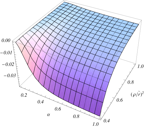
Figure 1: The energy density induced by the string, $\tilde{r}^{6}\langle{T}_{0}^{0}\rangle_{\mathrm{s}}$, as a function of $\alpha$ and $y=(\rho/\tilde{r})^{2}$ for $q=3$, $\gamma=1/3$.

In figure 2, we have presented the dependence of the part in the energy density induced by the string, on $y=(\rho/\tilde{r})^{2}$ for different values of the parameter $q$ (the numbers near the curves). The corresponding values of the parameter $\gamma$ are found from condition (45). The graphs are plotted for the value of the global monopole parameter $\alpha=0.5$. Note that in the cases $q=1,2$ the corresponding energy density vanishes.

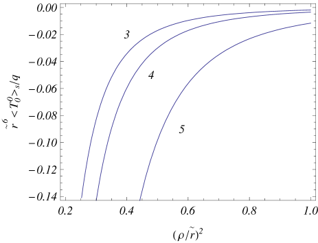
Figure 2: The dependence of the energy density induced by the string, $\tilde{r}^{6}\langle T_{0}^{0}\rangle_{\mathrm{s}}/q$, as a function of $y=(\rho/\tilde{r})^{2}$ for $\alpha=0.5$. The numbers near the curves correspond to the values of the parameter $q$.

The VEV of the radial component of the energy-momentum tensor will be given by

$$\langle T_{rr}(x)\rangle=\frac{1}{2\alpha}\lim_{x^{\prime}\rightarrow x}\mathrm{Tr}\left[{\hat{r}}\cdot{\vec{\gamma}}\left(\partial_{r}-\partial_{r^{\prime}}\right)\right]S_{F}(x,x^{\prime})\ ,$$ (66)

where we have used $D_{r}=\partial_{r}$ and ${\tilde{\sigma}}_{r}={\hat{r}}\cdot{\vec{\gamma}}/\alpha$. Expressing the Feynman propagator in terms of the Euclidean Green function, we can write:

$$\langle T_{rr}(x)\rangle=-\frac{1}{2\alpha}\lim_{x^{\prime}\rightarrow x}\mathrm{Tr}\left[{\hat{r}}\cdot{\vec{\gamma}}\left(\partial_{r}-\partial_{r^{\prime}}\right){\not{}D}{\mathcal{D}}_{E}(x^{\prime},x)\right]\ .$$ (67)

At this point we can make a similar analysis as we did in the calculation of the VEV of the energy density. For the $k=0$ component of (53), the only non-vanishing contributions coming from the product of $\gamma^{r}$ by (24), are given by the second, third and fourth terms of the latter. So, we may take for this component $\varphi^{\prime}=\varphi$. As a consequence the corresponding vacuum average again coincides with the one in the absence of string and magnetic flux. So, let us now proceed the calculation of the new contributions for the above VEV due to the terms with $k\geqslant 1$ in (53):

$$\langle T_{rr}(x)\rangle_{\mathrm{s}}=-\frac{1}{2\alpha}\lim_{x^{\prime}\rightarrow x}\mathrm{Tr}\left[{\hat{r}}\cdot{\vec{\gamma}}\left(\partial_{r}-\partial_{r^{\prime}}\right){\not{}D}{\mathcal{D}}_{E}^{(k\geqslant 1)}(x,x^{\prime})\right]\ .$$ (68)

Because of some simplifications that appear in this calculation, it is possible to observe that the only non-vanishing contribution comes from the second term on the right-hand side of (24) and one finds

$$\langle T_{rr}(x)\rangle_{\mathrm{s}}=\frac{1}{2}\lim_{x^{\prime}\rightarrow x}\mathrm{Tr}\left[\partial_{r}(\partial_{r}-\partial_{r^{\prime}})-\frac{\alpha+\kappa^{(\sigma)}}{\alpha r^{2}}\right]{\mathcal{D}}_{E}^{(k\geqslant 1)}(x,x^{\prime})\ .$$ (69)

Now substituting (53) into (69), and using relation (62), we can see that

$$\langle T_{r}^{r}\rangle_{\mathrm{s}}=\langle T_{0}^{0}\rangle_{\mathrm{s}}.$$ (70)

The calculation of the component $\langle T_{\rho\rho}\rangle$ is formally given by

$$\langle T_{\rho\rho}\rangle=\frac{1}{2}\lim_{x^{\prime}\rightarrow x}\mathrm{Tr}\left[{\tilde{\sigma}}_{\rho}(\partial_{\rho}-\partial_{\rho^{\prime}})\right]S_{F}(x,x^{\prime})\ ,$$ (71)

where we have used $D_{\rho}=\partial_{\rho}$. Expressing the Feynman propagator in terms of the Green function, and analyzing the $k=0$ component of (53), we conclude, after a careful analysis, that this component provides the same vacuum average as in the absence of string and magnetic flux. The only non-vanishing contributions to the parts in the VEV due to the string and magnetic flux come from the last two terms on the right-hand side of (24):

$$\langle T_{\rho}^{\rho}(x)\rangle_{\mathrm{s}}=\frac{1}{2}\lim_{x^{\prime}\rightarrow x}\mathrm{Tr}\left[\partial_{\rho}(\partial_{\rho}-\partial_{\rho^{\prime}})+\frac{q-1}{2\rho^{2}}-\frac{q\gamma_{5}}{\rho^{2}}(i\partial_{\varphi}+{\bar{N}}+\gamma)\right]{\mathcal{D}}_{E}^{(k\geqslant 1)}(x,x^{\prime})\ ,$$ (72)

where $\gamma=(q-1)/2q$. Substituting the expression for the Green function, and after a long calculation, we obtain for VEV of $T_{\rho}^{\rho}$ the same expression as obtained for $T_{0}^{0}$, given in (60):

$$\langle T_{\rho}^{\rho}\rangle_{\mathrm{s}}=\langle T_{0}^{0}\rangle_{\mathrm{s}}.$$ (73)

The other components of the VEV for the energy-momentum tensor are found from the covariant continuity equation $\nabla_{A}\langle T_{B}^{A}\rangle=0$. For the geometry under consideration this equation reduces to the following two relations

$$\langle T_{\theta}^{\theta}\rangle = \langle T_{\phi}^{\phi}\rangle=\left(1+\frac{r}{2}\partial_{r}\right)\langle T_{r}^{r}\rangle\ ,$$

$$\langle T_{\varphi}^{\varphi}\rangle = \partial_{\rho}(\rho\langle T_{\rho}^{\rho}\rangle)\ .$$ (74)

By using formulae (70), (73), (74), it can be checked that the part in the VEV of the energy-momentum tensor induced by the string and magnetic flux is traceless, $\langle T_{A}^{A}\rangle_{\mathrm{s}}=0$, and the trace anomaly is contained in the pure global monopole part only.

Having obtained the complete expressions for the VEVs of all components of the fermionic energy-momentum tensor induced by the cosmic string and magnetic flux, we let for the next section the analysis of the general case, where there is no more relation between the magnetic flux and the parameter associated with the cosmic string.

4 General case

4.1 Green function

In order to evaluate the vacuum expectation value of the energy-momentum tensor induced by the magnetic flux and cosmic string for general values of the parameters $b$ and $\gamma$, we shall subtract from the heat kernel (41) the corresponding heat kernel in the absence of cosmic string and taking $\gamma=0$. Denoting by ${\mathcal{K}}_{\mathrm{sub}}(x,x^{\prime};s)$ the subtracted heat kernel and introducing rescaled coordinates $\tilde{\varphi}=b\varphi$ and $\tilde{r}=r/\alpha$, we have

$${\mathcal{K}}_{\mathrm{sub}}(x,x^{\prime};s) = \frac{\alpha^{-2}}{32\pi^{3/2}\sqrt{\tilde{r}\tilde{r}^{\prime}}}\frac{e^{-\tilde{{\mathcal{V}}}/4s}}{s^{5/2}}\sum_{\sigma=0,1}\sum_{j,m_{j}}I_{\nu_{\sigma}}\left(\frac{\tilde{r}\tilde{r}^{\prime}}{2s}\right)$$ (77)

$$\times\sum_{n}\sum_{\delta}\left[qe^{iNq\Delta\tilde{\varphi}}I_{q|\mu_{\delta}|}\left(\frac{\rho\rho^{\prime}}{2s}\right)e^{iqn{\Delta}\tilde{\varphi}}-I_{n}\left(\frac{\rho\rho^{\prime}}{2s}\right)e^{in{\Delta}\tilde{\varphi}}\right]$$

$$\times\left(\begin{array}[]{cc}C_{j,m_{j}}^{\sigma}(\Omega,\Omega^{\prime})&\delta C_{j,m_{j}}^{\sigma}(\Omega,\Omega^{\prime})\\ \delta C_{j,m_{j}}^{\sigma}(\Omega,\Omega^{\prime})&C_{j,m_{j}}^{\sigma}(\Omega,\Omega^{\prime})\end{array}\right)\ ,$$

where ${\Delta}\tilde{\varphi}=\tilde{\varphi}-\tilde{\varphi}^{\prime}$ and

$$\tilde{\mathcal{V}}=\Delta\tau^{2}+\rho^{2}+\rho^{\prime}{}^{2}+\tilde{r}^{2}+\tilde{r}^{\prime}{}^{2}\ .$$ (78)

Though the contribution of the separate terms in square brackets of (77) to the Green function is divergent in the coincidence limit, the part of the Green function corresponding to the subtracted heat kernel (77) is finite in the coincidence limit for points away from the string core. This follows also from general arguments. For points outside the string core the electromagnetic field is zero and the local geometry is the same as that in the case when the global monopole is present only. Hence, the divergences in the Green function in the coincidence limit are the same in these two situations.

To provide a more convenient expression for the subtracted heat kernel, for the summation over $n$ we apply the Abel-Plana formula in the form

$$\sum_{n=n_{\pm}}^{\infty}F(n\pm\beta)=\int_{0}^{\infty}du\,F(u)+i\int_{0}^{\infty}du\sum_{\lambda=\pm 1}\frac{\lambda F(i\lambda u)}{e^{2\pi(u\pm i\lambda\beta)}-1},$$ (79)

where $n_{+}=0$, $n_{-}=1$, and $0<\beta<1$. This generalization of the Abel-Plana formula with the upper sign is given in [26] and the formula with the lower sign is easily obtained from the upper sign case by redefining $n\rightarrow n+1$. Note that formula (79) is also obtained from the generalized Abel-Plana formula (see [27]).

Defining the sum

$$S_{q,\gamma}^{(\delta)}(z,{\Delta}\tilde{\varphi})=e^{iNq\Delta\tilde{\varphi}}\sum_{n}qI_{q|\mu_{\delta}|}(z)e^{iqn{\Delta}\tilde{\varphi}},$$ (80)

and using formula (79), after some intermediate steps we find

$$S_{q,\gamma}^{(\delta)}(z,{\Delta}\tilde{\varphi}) = 2e^{i(N-\beta_{\delta})q{\Delta}\tilde{\varphi}}\bigg{[}\int_{0}^{\infty}duI_{u}(z)\cos(u{\Delta}\tilde{\varphi})$$ (81)

$$+\frac{1}{\pi}\int_{0}^{\infty}du\sinh(u\pi)K_{iu}(z)\sum_{\lambda=\pm 1}\frac{e^{-\mathrm{sgn}(\beta_{\delta})\lambda u{\Delta}\tilde{\varphi}}}{e^{2\pi(u/q+i\lambda|\beta_{\delta}|)}-1}\bigg{]},$$

where $K_{\nu}(z)$ is the MacDonald function and we have defined

$$\beta_{\delta}=\delta(q-1)/2q-\gamma.$$ (82)

To the sum over $n$ with the second term in the square brackets of (77) we apply the Abel-Plana formula in the standard form. This gives

$$S(z,{\Delta}\tilde{\varphi}) = \sum_{n}I_{n}\left(z\right)e^{in{\Delta}\tilde{\varphi}}=2\int_{0}^{\infty}duI_{u}(z)\cos(u{\Delta}\tilde{\varphi})$$ (83)

$$+\frac{4}{\pi}\int du\sinh(\pi u)K_{iu}(z)\frac{\cosh(u{\Delta}\tilde{\varphi})}{e^{2\pi u}-1}\ .$$

The subtracted Green function, ${\mathcal{D}}_{\mathrm{sub}}(x,x^{\prime})$, that we shall use to calculate the vacuum polarization effects induced by the cosmic string and magnetic flux, is obtained from formulae (44) and (77):

$${\mathcal{D}}_{\mathrm{sub}}(x,x^{\prime}) = \frac{\sqrt{2}\alpha^{-2}}{16\pi^{3/2}\sqrt{\tilde{r}\tilde{r}^{\prime}}}\int_{0}^{\infty}du\ u^{1/2}e^{-u\tilde{{\mathcal{V}}}/2}\bigg{[}\sum_{\delta}S_{q,\gamma}^{(\delta)}(u\rho\rho^{\prime},{\Delta}\tilde{\varphi})-S(u\rho\rho^{\prime},{\Delta}\tilde{\varphi})\bigg{]}$$ (86)

$$\times\sum_{\sigma=0,1}\sum_{j,m_{j}}I_{\nu_{\sigma}}\left(u\tilde{r}\tilde{r}^{\prime}\right)\left(\begin{array}[]{cc}C_{j,m_{j}}^{\sigma}(\Omega,\Omega^{\prime})&\delta C_{j,m_{j}}^{\sigma}(\Omega,\Omega^{\prime})\\ \delta C_{j,m_{j}}^{\sigma}(\Omega,\Omega^{\prime})&C_{j,m_{j}}^{\sigma}(\Omega,\Omega^{\prime})\end{array}\right),\$$

where $\tilde{{\mathcal{V}}}$ is defined by relation (78). The divergent contributions from the separate terms in the square brackets of (86) come from the first integrals on the right-hand sides of formulae (81) and (83). Now we see that after the application of the Abel-Plana formula these contributions are explicitly cancelled out in the subtracted Green function for ${\Delta}\tilde{\varphi}=0$.

4.2 Energy-momentum tensor

Having the subtracted Green function we can evaluate the VEV of the energy-momentum tensor on the base of formula (54). As in the special case discussed before, let us consider the part in the vacuum average of $T_{0}^{0}$ induced by the string and flux:

$$\langle T_{0}^{0}(x)\rangle_{\mathrm{s}}=\lim_{x^{\prime}\rightarrow x}\mathrm{Tr}\left[\gamma_{0}\partial_{0}{\not{}D}{\mathcal{D}}_{\mathrm{sub}}(x,x^{\prime})\right]\ .$$ (87)

Being ${\mathcal{D}}_{\mathrm{sub}}(x,x^{\prime})$ finite at the coincidence limit, we can interchange the differential operator and the integral over $u$. Moreover, terms linear in time derivative acting on the exponential factor of the subtracted heat kernel, $e^{-\tilde{{\mathcal{V}}}/4s}$, produce a term linear in $\Delta\tau$, which goes to zero at the coincidence limit. The only term that survives is the one obtained by the second time derivative. So on the basis of these information, we may write:

$$\langle T_{0}^{0}(x)\rangle_{\mathrm{s}}=\lim_{x^{\prime}\rightarrow x}\mathrm{Tr}\partial_{\tau}^{2}{\mathcal{D}}_{\mathrm{sub}}(x,x^{\prime})=\lim_{x^{\prime}\rightarrow x}\mathrm{Tr}\int_{0}^{\infty}ds\ \partial_{\tau}^{2}{\mathcal{K}}_{\mathrm{sub}}(x,x^{\prime};s)\ .$$ (88)

Developing all the calculations needed and defining a new integration variable, $v=u\tilde{r}^{2}$, we obtain:

$$\langle T_{0}^{0}\rangle_{\mathrm{s}} = -\frac{\sqrt{2}\alpha^{-2}}{16\pi^{5/2}\tilde{r}^{6}}\int_{0}^{\infty}dv\ v^{3/2}e^{-(1+y)v}\sum_{\sigma=0,1}\sum_{j}(j+1/2)$$ (89)

$$\times I_{\nu_{\sigma}}\left(v\right)\sum_{n}\bigg{[}\sum_{\delta=\pm 1}qI_{q|\mu_{\delta}|}(yv)-2I_{n}\left(yv\right)\bigg{]}\,.$$

with $y$ defined by (61).

An equivalent form for $\langle T_{0}^{0}\rangle_{\mathrm{s}}$ is obtained by using formulae (81) and (83) with ${\Delta}\tilde{\varphi}=0$:

$$\langle T_{0}^{0}\rangle_{\mathrm{s}}=-\frac{\sqrt{2}}{16\pi^{5/2}\alpha^{2}\tilde{r}^{6}}\int_{0}^{\infty}dv\ v^{3/2}e^{-(1+y)v}\sum_{l=1}^{\infty}l\left[I_{l/\alpha-1/2}(v)+I_{l/\alpha+1/2}(v)\right]F_{q,\gamma}(yv),$$ (90)

In this formula we have introduced the notation

$$F_{q,\gamma}(z)=\sum_{\delta=\pm 1}S_{q,\gamma}^{(\delta)}\left(z,0\right)-2S\left(z,0\right)=\frac{2}{\pi}\int_{0}^{\infty}du\sinh(u\pi)K_{iu}(z)G_{q,\gamma}(u).$$ (91)

where

$$G_{q,\gamma}(u)=\sum_{\delta=\pm 1}\sum_{\lambda=\pm 1}\frac{1}{e^{2\pi(u/q+i\lambda|\beta_{\delta}|)}-1}-\frac{4}{e^{2\pi u}-1},$$ (92)

and $\beta_{\delta}$ is defined by (82). Note that, as it follows from (92), the VEV of the energy-momentum tensor does not depend on the sign of the fractional part of the magnetic flux.

We could have obtained the second relation in (91) by applying to the series over $n$ in the definitions of $S_{q,\gamma}^{(\delta)}\left(z,0\right)$ and $S\left(z,0\right)$ the summation formula

$$\sum_{n=-\infty}^{\infty}F(|n+\beta|)=2\int_{0}^{\infty}du\,F(u)+i\int_{0}^{\infty}du\sum_{\lambda=\pm 1}\frac{F(iu)-F(-iu)}{e^{2\pi(u+i\lambda\beta)}-1},$$ (93)

which directly follows from (79). Note that for this formula the restriction $0<\beta<1$ is not necessary and it holds for any real value of the parameter $\beta$. The Abel-Plana formula in its standard form (see, for instance, [28]) is obtained from here taking $\beta=0$.

The components $\langle T_{rr}\rangle_{\mathrm{s}}$ and $\langle T_{\rho\rho}\rangle_{\mathrm{s}}$ are found by the formulae similar to (69) and (72) with the replacement ${\mathcal{D}}_{E}^{(k\geqslant 1)}(x,x^{\prime})\rightarrow{\mathcal{D}}_{\mathrm{sub}}(x,x^{\prime})$. The resulting expressions for $\langle T_{r}^{r}\rangle_{\mathrm{s}}$ and $\langle T_{\rho}^{\rho}\rangle_{\mathrm{s}}$ are obtained from formula (89) for the energy density by the replacement $I_{\nu_{\sigma}}\left(z\right)\rightarrow[I_{\nu_{\sigma}+n_{\sigma}}\left(z\right)+I_{\nu_{\sigma}}\left(z\right)]/2$ with $z=\tilde{r}^{2}/2s$ in the case of $\langle T_{r}^{r}\rangle_{\mathrm{s}}$ and by the replacement $I_{q|\mu_{\delta}|}\left(z\right)\rightarrow[I_{q|\mu_{\delta}|+\delta\mu_{\delta}/|\mu_{\delta}|}\left(z\right)+I_{q|\mu_{\delta}|}\left(z\right)]/2$ with $z=\rho^{2}/2s$ in the case of $\langle T_{\rho}^{\rho}\rangle_{\mathrm{s}}$. After summation over $\sigma$ and $\delta$ we see that $\langle T_{r}^{r}\rangle_{\mathrm{s}}=\langle T_{\rho}^{\rho}\rangle_{\mathrm{s}}=\langle T_{0}^{0}\rangle_{\mathrm{s}}$. Other components are found from relations (74). It can be additionally checked that the resulting tensor is traceless.

Now we consider the behavior of the string induced part in the VEV of the energy density in the asymptotic regions of the parameter $y$. For large values of this parameter, $y\gg 1$, introducing in (90) a new integration variable $z=yv$ and expanding the integrand over $1/y$, to the leading order we find

$$\langle T_{0}^{0}\rangle_{\mathrm{s}}\approx-\frac{(\tilde{r}/\rho)^{2/\alpha-2}}{4^{2+1/\alpha}\pi^{3}\alpha^{2}\rho^{6}}\int_{0}^{\infty}du\,G_{q,\gamma}(u)\frac{\sinh(u\pi)|\Gamma(1/\alpha+2+iu)|^{2}}{\Gamma(1/\alpha+1/2)\Gamma(1/\alpha+5/2)},$$ (94)

for $\rho\gg\tilde{r}$. In particular, for $\alpha<1$ the expectation value induced by the string and magnetic flux vanishes on the core of the global monopole. From formula (94) it follows that at large distances from the string, the string induced energy density is suppressed by the factor $(\tilde{r}/\rho)^{2/\alpha-2}$ with respect to the corresponding quantity in the absence of the global monopole.

As the vacuum expectation value given by (90) diverges on the string core corresponding to $y=0$, in the limit $y\ll 1$ the main contribution into the sum over $l$ comes from large values $l$ and we can use the uniform asymptotic expansion for the functions $I_{l/\alpha\pm 1/2}(v)$. As the next step, we replace the summation over $l$ by the integration. After some intermediate calculations, for the vacuum average of the energy density induced by the presence of the string and magnetic flux to the leading order one finds

$$\langle T_{0}^{0}\rangle_{\mathrm{s}}\approx-\frac{1}{60\pi^{3}\rho^{6}}\int_{0}^{\infty}du\,u(u^{2}+1)(u^{2}+4)G_{q,\gamma}(u).$$ (95)

The expression on the right-hand side of this formula does not depend on the parameter $\alpha$ and coincides with the corresponding quantity in the geometry of a cosmic string with magnetic flux when the global monopole is absent ($\alpha=1$, see below). This means that near the cosmic string the most relevant contribution to the vacuum expectation value comes from the string itself.

For small values of the parameter $\alpha$, corresponding to strong gravitational field, the order of the modified Bessel functions in (90) is large. Again, replacing these functions by the corresponding uniform asymptotic expansion we can estimate the integral over $v$ by the Laplace method. In this way it can be seen that the main contribution comes from $l=1$ term and one finds

$$\langle T_{0}^{0}\rangle_{\mathrm{s}}\approx-\frac{\exp[-(1/\alpha)\ln(1+2y+2\sqrt{y(1+y)})]}{16\pi^{3}\tilde{r}^{6}\alpha^{3}y^{3/2}(1+y)}\int_{0}^{\infty}du\sinh(u\pi)G_{q,\gamma}(u).$$ (96)

As we see, in this limit the vacuum expectation values are exponentially suppressed. The similar feature takes place for the VEV of the energy-momentum tensor and the fermionic condensate induced in the global monopole bulk by the presence of boundaries on which the fermionic field obeys the MIT bag boundary condition [29].

In the case when the global monopole is absent, $\alpha=1$, the summation over $l$ in the expression (90) for $\langle T_{0}^{0}\rangle_{\mathrm{s}}$ can be done by using the formula [23] $\sum_{l=0}^{\infty}(2l+1)I_{l+1/2}(x)=e^{x}\sqrt{2x/\pi}$. Redefining a new variable $z=yv$ we have

$$\langle T_{0}^{0}\rangle_{\mathrm{s}}=-\frac{1}{8\pi^{3}\rho^{6}}\int_{0}^{\infty}dz\ z^{2}e^{-z}F_{q,\gamma}(z)\ .$$ (97)

By taking into account the expression (91) for $F_{q,\gamma}(z)$, the integral over $z$ is evaluated explicitly using the formula from [23]. After some intermediate steps, we arrive to the following expression:

$$\langle T_{0}^{0}\rangle_{\mathrm{s}}=-\frac{1}{60\pi^{3}\rho^{6}}\int_{0}^{\infty}du\,u(u^{2}+1)(u^{2}+4)G_{q,\gamma}(u).$$ (98)

Note that by making use of the formula

$$A_{m}(q,\beta) = \int_{0}^{\infty}du\,u^{2m-1}\left[\sum_{\lambda=\pm 1}\frac{1}{e^{2\pi(u/q+i\lambda\beta)}-1}-\frac{2}{e^{2\pi u}-1}\right]$$ (99)

$$= \frac{(-1)^{m-1}}{2m}\left[q^{2m}B_{2m}(\beta)-B_{2m}\right],$$

where $B_{2m}(\beta)$ and $B_{2m}$ are the Bernoulli polynomials and Bernoulli numbers respectively, the energy density is also presented in the form

$$\langle T_{0}^{0}\rangle_{\mathrm{s}}=-\frac{1}{60\pi^{3}\rho^{6}}\sum_{\delta=\pm 1}\left[A_{3}(q,|\beta_{\delta}|)+5A_{2}(q,|\beta_{\delta}|)+4A_{1}(q,|\beta_{\delta}|)\right].$$ (100)

For the case $(q-1)/(2q)>\gamma$ the explicit calculation by this formula gives the result

$$\langle T_{0}^{0}\rangle_{\mathrm{s}} = -\frac{\pi^{-3}\rho^{-6}}{241920}[367+189q^{2}(-1+12\gamma^{2})-21q^{4}(7-120\gamma^{2}+240\gamma^{4})$$ (101)

$$+q^{6}(-31+588\gamma^{2}-1680\gamma^{4}+1344\gamma^{6})].$$

In the presence of both chiralities the result given by (101) should be doubled and it coincides with the formula derived in [24]. Considering the special case given by (45), from (101) we obtain formula (64). Hence, though we have derived formula (64) for integer values of $q$, we see that it is valid for non-integer $q$ as well.

5 Conclusions

In this paper we investigate quantum vacuum effects for a massless fermionic field induced by a composite topological defect in a six dimensional spacetime. The spacetime is a direct product of the two dimensional cosmic string and three dimensional global monopole geometries. The corresponding heat kernel is constructed and on the base of this, the Green function is evaluated for a field with positive chirality. The consideration of a negative chirality field is similar. As the corresponding geometry with a global monopole and in the absence of a cosmic string was investigated previously in [16], here we mainly concentrate on the effects induced by the cosmic string and magnetic flux along the core of the string. With this aim, the complete Green function is presented as the sum of two terms. The first one contains information only on the global monopole defect and the second one is induced by the presence of the cosmic string and magnetic flux. For points away from the string the second term in the Green function is finite in the coincidence limit and can be directly used for the evaluation of the vacuum expectation value of the energy-momentum tensor.

In section 3 we have considered a special case when the parameters of the cosmic string and magnetic flux are connected by relation (45) and $q$ is an integer. In this case the summation over $n$ in the mode-sum for the heat kernel can be done explicitly and the Euclidean Green function is presented in the form (53). The vacuum expectation value of the energy-momentum tensor is constructed from the Feynman propagator by making use of formula (54). The energy density induced by the string and magnetic flux is given by formula (60). The corresponding vacuum stresses along $r$- and $\rho$-directions coincide with energy density. The other components of the vacuum stress are found from the covariant continuity equation for the energy-momentum tensor. We have explicitly checked that the part of the energy-momentum tensor induced by the string and flux is traceless.

The Green function and the vacuum expectation value of the energy-momentum tensor for the general case of the string and flux parameters are discussed in section 4. By using the Abel-Plana summation formula, the corresponding subtracted Green function is presented in the form (86) where the parts giving the divergences in the coincidence limit are explicitly cancelled out. Further, this Green function is used for the evaluation of the corresponding energy-momentum tensor. The vacuum energy density is given by formula (90) and, as for the special case, the stresses along $r$- and $\rho$-directions coincide with energy density. The remained components are found from relations (74). As for pure cosmic string geometry, the VEV of the energy-momentum tensor depends only on the fractional part of the magnetic flux and is an even function of this parameter. We have investigated the vacuum energy-momentum tensor in asymptotic regions of the parameters. At large distances from the string, $\rho\gg\tilde{r}$, the leading term of the asymptotic expansion of the energy density is given by formula (94). In this case the string induced energy density is suppressed by the factor $(\tilde{r}/\rho)^{2/\alpha-2}$ with respect to the corresponding quantity in the absence of the global monopole. For points near the string core, $\rho\ll\tilde{r}$, to the leading order the string induced part in the vacuum average coincides with the corresponding quantity in the geometry of a cosmic string with magnetic flux when the global monopole is absent. For small values of the parameter $\alpha$, corresponding to strong gravitational fields, the vacuum expectation values are exponentially suppressed.

References

• [1] A. Vilenkin and E.P.S. Shellard, Cosmic Strings and Other Topological Defects (Cambridge University Press, Cambridge, UK, 1994).
• [2] S. Sarangi and S.H.H. Tye, Phys. Lett. B 536, 185 (2002); E.J. Copeland and R.C. Myers, J. Polchinski, JHEP 0406, 013 (2004); G. Dvali and A. Vilenkin, JCAP 0403 (2004) 010; A. Achúcarro and J. Urrestilla, JHEP 0408, 050 (2004).
• [3] B. Linet, Phys. Rev. D 35, 536 (1987); A. G. Smith, in Symposium on the Formation and Evolution of Cosmic String, edited by G.W. Gibbons, S.W. Hawking and T. Vachaspati (Cambridge University Press, Cambridge, England, 1989); M.E. X. Guimarães and B. Linet, Class. Quantum Grav. 10, 1665 (1993); V.B. Bezerra and E.R. Bezerra de Mello, Class. Quantum Grav. 11, 457 (1994); E.R. Bezerra de Mello, Class. Quantum Grav. 11, 1415 (1994).
• [4] P.C. Davies and V. Sahni, Class. Quantum Grav. 5, 1 (1987); T. Souradeep and V. Sahni, Phys. Rev. D 46, 1616 (1992).
• [5] V.P. Frolov and E.M. Serebriany, Phys. Rev. D 15, 3779 (1287); B. Linet, J. Math. Phys. 36, 3694 (1995); E.S. Moreira Jnr., Nucl. Phys. B 451, 365 (1995); V.B. Bezerra and N.R. Khusnutdinov, Class. Quantum Grav. 23, 3449 (2006).
• [6] J.S. Dowker, Phys. Rev. D 36, 3742 (1987). M.E.X. Guimarães and B. Linet, Commun. Math. Phys. 165, 297 (1994); L. Sriramkumar, Class. Quantum Grav. 18, 1015 (2001); J. Spinelly and E.R. Bezerra de Mello, Class. Quantum Grav. 20, 874 (2003); J. Spinelly and E. R. Bezerra de Mello, Int. J. Mod. Phys. A 17, 4375 (2002); J. Spinelly and E.R. Bezerra de Mello, Int. J. Mod. Phys. D 13, 607 (2004).
• [7] I. Brevik and T. Toverud, Class. Quantum Grav. 12, 1229 (1995); I. Brevik and T. Toverud, Phys. Rev. D 51, 691 (1995); N.R. Khusnutdinov and M. Bordag, Phys. Rev. D 59, 064017 (1999).
• [8] E.R. Bezerra de Mello, V.B. Bezerra, A.A. Sharian, and A.S. Tarloyan, Phys. Rev. D 74, 025017 (2006); E.R. Bezerra de Mello, V.B. Bezerra and A.A. Sharian, Phys. Lett. B 645, 245 (2007).
• [9] V.A. Rubakov, Phys. Usp. 44, 871 (2001); R. Maartens, Living Rev. Relativ. 7, 7 (2004).
• [10] L. Randall and R. Sundrum, Phys. Rev. Lett. 83, 3370 (1999); L. Randall and R. Sundrum, Phys. Rev. Lett. 83, 4690 (1999).
• [11] A.G. Cohen and D.B. Kaplan, Phys. Lett. B 470, 52 (1999); R. Gregory, Phys. Rev. Lett. 84, 2564 (2000).
• [12] E. Roessl and M. Shaposnikov, Phys. Rev. D 66, 084008 (2002); I. Cho and A. Vilenkin, Phys. Rev. D 69, 045005 (2004).
• [13] I. Olasagasti and A. Vilenkin, Phys. Rev. D 62, 044014 (2000); T. Gherghetta, E. Roessl, and M. Shaposnikov, Phys. Lett. B 491, 353 (2000); I. Olasagasti, Phys. Rev. D 63, 124016 (2001); K. Benson and I. Cho, Phys. Rev. D 64, 065026 (2001)
• [14] I. Cho and A. Vilenkin, Phys. Rev. D 68, 025013 (2003).
• [15] E.R. Bezerra de Mello, Phys. Rev. D 73, 105015 (2006).
• [16] E.R. Bezerra de Mello, Phys. Rev. D 76, 125021 (2007).
• [17] E.R. Bezerra de Mello and A.A. Saharian, Phys. Let. B 642, 129 (2006).
• [18] E.M. Serebryanyi, Theor. Math. Phys. 64, 846 (1985); M. Bordag and K. Kirsten, Phys. Rev. D 60, 105019 (1999); Yu.A. Sitenko, Phys. Rev. D 60, 125017 (1999); N. Graham, V. Khemani, M. Quandt, O. Schroeder, and H. Weigel, Nucl. Phys. B 707, 233 (2005).
• [19] M.R. Douglas and S. Kachru, Rev. Mod. Phys. 79, 733 (2007).
• [20] J.D. Bjorken and S.D. Drell, Relativistic Quantum Mechanics (McGraw-Hill, New York, 1964).
• [21] R.N. Mohapatra and A. Pérez-Lorenzana, Phis. Rev. D 67, 075015 (2003).
• [22] N.D. Birrell and P.C.W. Davies. Quantum Fields in Curved Space (Cambridge University Press, Cambridge, England, 1982).
• [23] A.P. Prudnikov, Yu.A. Brychkov, and O.I. Marichev, Integrals and Series (Gordon and Breach, New York, 1986), Vol. 2.
• [24] J. Spinelly and E.R. Bezerra de Mello, arXiv:0802.4401[hep-th].
• [25] M. Abramowitz and I.A. Stegun, Handbook of Mathematical Functions (National Bureau of Standards, Washington, DC, 1964).
• [26] N. Inui, J. Phys. Soc. Japan 72, 1035 (2003).
• [27] A.A. Saharian, ”The generalized Abel-Plana formula with applications to Bessel functions and Casimir effect,” Preprint ICTP/2007/082; arXiv: 0708.1187.
• [28] V.M. Mostepanenko and N.N. Trunov, The Casimir Effect and Its Applications (Oxford University Press, Oxford, 1997).
• [29] A.A. Saharian and E.R. Bezerra de Mello, J. Phys. A 37, 3543 (2004); A.A. Saharian and E.R. Bezerra de Mello, Int. J. Mod. Phys. A 20, 2380 (2005); E.R. Bezerra de Mello and A.A. Saharian, Class. Quantum Grav. 23, 4673 (2006).