Quantum Stephani Universe in vicinity of the symmetry center

Abstract

We study a class of spherically symmetric Stephani cosmological models in the presence of a self-interacting scalar field in both classical and quantum domains. We discuss the construction of ‘canonical’ wave packets resulting from the solutions of a class of Wheeler-DeWitt equations in the Stephani Universe. We suggest appropriate initial conditions which result in wave packets containing some desirable properties, most importantly good classical and quantum correspondence. We also study the situation from de-Broglie Bohm interpretation of quantum mechanics to recover the notion of time and compare the classical and Bohmian results. We exhibit that the usage of the canonical prescription and appropriate choices of expansion coefficients result in the suppression of the quantum potential and coincidence between classical and Bohmian results. We show that, in some cases, contrary to Friedmann-Robertson-Walker case, the bound state solutions also exist for all positive values of the cosmological constant.

Pacs: 98.80.Qc, 04.40.Nr, 04.60.Ds;

1 Introduction

In recent years observations show that the expansion of the Universe is accelerating in the present epoch [1] contrary to Friedmann-Robertson-Walker (FRW) cosmological models, with non-relativistic matter and radiation. Some different physical scenarios using exotic form of matter have been suggested to resolve this problem [2, 3, 4, 5, 6, 7]. In fact the presence of exotic matter is not necessary to drive an accelerated expansion. Instead we can relax the assumption of the homogeneity of space, leaving the isotropy with respect to one point. The most general class of non-static, perfect fluid solutions of Einstein’s equations that are conformally flat is known as the “Stephani Universe” [8, 9]. This model can be embedded in a five-dimensional flat pseudo-Euclidean space [8, 10, 11] and its three dimensional spatial sections are homogeneous and isotropic [12]. Recently, quantum spherically symmetric Stephani cosmological models in the presence of the perfect fluid have been studied in Refs. [13, 14]. In these works the Schutz’s variational formalism [15, 16] is applied to recover the notion of time and investigate the singularity avoidance at the quantum level.

The question of construction and interpretation of wave packets in quantum cosmology and its connection with classical cosmology has been attracting much attention in recent years. Moreover, numerous studies have been done to obtain a quantum theory for gravity and to understand its connection with classical physics.

In quantum cosmology, in analogy with ordinary quantum mechanics, one is generally concerned with the construction of wave functions by the superposition of the ‘energy eigenstates’ which would peak around the classical trajectories in configuration space, whenever such classical-quantum correspondence is mandated by the nature of the problem. However, contrary to ordinary quantum mechanics, a parameter describing time is absent in quantum cosmology. Therefore, the initial conditions would have to be expressed in terms of an intrinsic time parameter, which in the case of the Wheeler-DeWitt (WDW) equation could be taken as the local scale factor for the three geometry [17]. Also, since the sign of the kinetic term for the scale factor is negative, a formulation of the Cauchy problem for the WDW equation is possible. The existence of such a sign is one of the exclusive features of gravity with many other interesting implications.

The construction of wave packets resulting from the solutions of the WDW equation has been a common feature of some research works in quantum cosmology [18, 19, 20, 21, 22]. In particular, in references [21, 22, 23] the construction of wave packets in a Friedmann Universe is presented in detail and appropriate boundary conditions are motivated. Generally speaking, one of the aims of these investigations has been to find wave packets whose probability distributions coincide with the classical paths obtained in classical cosmology. In these works, the authors usually consider theories in which a self interacting scalar field is coupled to gravity in a Robertson-Walker type Universe. The solutions are obtained such that the following desirable properties are satisfied. There should be a good classical-quantum correspondence, which means that the wave packet should centered around the classical path, the crest of the wave packet should follow as closely as possible the classical path, and to each distinct classical path there should correspond a wave packet with the above properties. Recently, a general prescription has been suggested by Gousheh et al [22] for constructing the ‘canonical’ wave packets which contain all above desired properties. They showed that there always exists a “canonical initial slope” (CIS) for a given initial wave function, which optimizes some desirable properties of the resulting wave packet, most importantly good classical-quantum correspondence.

In this paper we deal with the subject of “initial condition” which is an important problem in quantum cosmology. In fact, in classical cosmology we can uniquely determine the classical initial conditions subject to the zero energy condition. But in quantum cosmology since the underlying equation (WDW equation) is a hyperbolic differential equation, we are free to choose the initial wave function and the initial derivative of the wave function by choosing arbitrary expansion coefficients. These quantities (distributions) correspond to classical initial position and initial momentum, respectively. Therefore, although WDW equation allows us to use different choices of initial conditions upon choosing different expansion coefficients, these wave functions correspond to different classical situations. This also happens whenever WDW-like equation appears in other theories such as varying speed of light quantum cosmological models [23]. Hence, a legitimate question which arises is how we can construct a specific wave packet which completely corresponds to its unique classical counterpart? One possible solution is removing the arbitrariness of the expansion coefficients and defining a certain relation between them. In our previous investigations [22, 23] we discovered that given a particular choice of initial wave function, certain coefficients remain undetermined, and if we set the functional form of those coefficient to be the same as the determined ones, we obtain excellent classical and quantum correspondence.

Here, we are interested to study the Stephani Universe in the presence of a scalar field. First, we write the reduced action near symmetry center ($r\approx 0$) and find the corresponding hamiltonian. Then we obtain the Einstein’s equations and WDW equations in minisuperspace. These equations can be solved numerically with appropriate initial conditions. In particular, we use Spectral Method (SM) [24] as an accurate and stable numerical method for solving the quantum cosmology case which can be cast in the form of a hyperbolic PDE. The form of the scalar potential is chosen to contain some desirable properties like the cosmological constant, positive mass term in Taylor expansion, and to be bounded from below. Then, we construct the wave packets for various functional forms of the spatial curvature through the canonical prescription [22].

The paper is organized as follows: In Sec. 2, we outline the main problem which is a case of Stephani cosmology where the matter is taken to be a particular type of self-interacting scalar field. We derive the main equations both for the classical cosmology and the quantum cosmology. We begin Sec. 3 with a description of the Spectral Method [24] which is a robust numerical method, and then we review the general prescription of canonical wave packets. We then consider various cases and solve them in both classical and quantum cosmological domains. In Sec. 4, we find the corresponding Bohmian trajectories and compare the classical and quantum solutions. In Sec. 5, we draw some final conclusions.

2 The model

Let us start from the Einstein-Hilbert action plus a scalar field as

$$S=\frac{1}{2}\int_{M}d^{4}x\sqrt{-g}\,{\cal R}+2\int_{\partial M}d^{3}x\sqrt{h}\,h_{ab}\,K^{ab}+\int_{M}d^{4}x\sqrt{-g}\,\left(-\frac{1}{2}(\nabla\phi)^{2}-U(\phi)\right),$$ (1)

where $K^{ab}$ is the extrinsic curvature and $h_{ab}$ is the induced metric over the three-dimensional spatial hypersurface, which is the boundary $\partial M$ of the four dimensional manifold $M$ in units where $8\pi G=1$ [25]. The last term of (1) represents the scalar field contribution to the total action.

The metric in spherically symmetric Stephani Universe [8, 9, 12, 10, 26, 27] has the following form

$$ds^{2}=-N^{2}(r,t)dt^{2}+\frac{R^{2}(t)}{V^{2}(r,t)}\left[dr^{2}+r^{2}(d\theta^{2}+\sin^{2}\theta\,d\phi^{2})\right],$$ (2)

where

$$N(r,t)=F(t)\frac{\displaystyle R(t)}{\displaystyle V(r,t)}\frac{\displaystyle\partial}{\displaystyle\partial t}\left(\frac{\displaystyle V(r,t)}{\displaystyle R(t)}\right),$$ (3)

is the lapse function and the functions $V(r,t)$ and $F(t)$ are defined as

$$V(r,t) = 1+\frac{1}{4}k(t)r^{2},$$ (4)

$$F(t) = \frac{R(t)}{\sqrt{C^{2}(t)R^{2}(t)-k(t)}},$$ (5)

where $k$, $R$, and $C$ are arbitrary functions of time [28, 29]. Here, $k(t)$ plays the role of the spatial curvature and $R(t)$ is the Stephani version of the FRW scale factor. Although $k(t)$ is an arbitrary function of time in the Stephani model, assuming a power law relation between $R(t)$ and $k(t)$ makes the model solvable and is in agreement with the accelerating expansion of the Universe [13, 14, 27, 29, 30, 31]. However, some authors have used some thermodynamics relations to obtain a power law relation between these two variables [31]. Though in the spherical symmetric inhomogeneous models, the scalar field $\phi$ depends on both $r$ and $t$, we can consider it as an only function of time near the symmetry center $r\approx 0$ which means $\phi=\phi(t)$ [32, 33, 34].

By substituting the Stephani metric (2) in the action (1) and choosing the curvature function $k(t)$ in the form [13, 14, 27, 29, 30, 31]

$$k(t)=\beta R^{\gamma}(t),$$ (6)

after dropping the surface terms and with due attention to the form of the lapse function (3), the final reduced action near $r\approx 0$ takes the form

$$S=\int dt\left[-3\frac{\displaystyle\dot{R}^{2}R}{\displaystyle N}+3\beta\,N\,R^{1+\gamma}+N\,R^{3}\left(\frac{1}{2}\dot{\phi}^{2}-U(\phi)\right)\right].$$ (7)

Now choosing the gauge $N=1$ [28, 29], we have the following Lagrangian

$$L=-3\dot{R}^{2}R+3\beta R^{1+\gamma}+R^{3}\left(\frac{1}{2}\dot{\phi}^{2}-U(\phi)\right).$$ (8)

Therefore, in this limit, the Stephani Universe is equivalent to the FRW model where the curvature term can be chosen as an arbitrary function of time.

The Einstein’s equations for $r\approx 0$ resulting from above Lagrangian with the zero energy condition can be written as

$$3\left[\left(\frac{\dot{R}}{R}\right)^{2}+\beta R^{\gamma-2}\right] = \frac{\dot{\phi}^{2}}{2}+U(\phi),$$ (9)

$$2\left(\frac{\ddot{R}}{R}\right)+\left(\frac{\dot{R}}{R}\right)^{2}+\beta(1+\gamma)R^{\gamma-2} = -\frac{\dot{\phi}^{2}}{2}+U(\phi),$$ (10)

$$\ddot{\phi}+3\frac{\dot{R}}{R}\dot{\phi}+\frac{\partial U}{\partial\phi} = 0,$$ (11)

where dot represents differentiation with respect to time. We require the potential $U(\phi)$ to have natural characteristics for small $\phi$, so that we may identify the coefficient of $\frac{1}{2}\phi^{2}$ in its Taylor expansion as a positive mass squared $m^{2}$, and $U(0)$ as a cosmological constant $\Lambda$. An interesting choice of $U(\phi)$ with three free parameters is [19, 21, 22, 35, 36, 37]

$$U(\phi)=\Lambda+\frac{m^{2}}{2\alpha^{2}}\sinh^{2}(\alpha\phi)+\frac{b}{2\alpha^{2}}\sinh(2\alpha\phi).$$ (12)

In the above expression $m^{2}=\partial^{2}U/\partial\phi^{2}|_{\phi=0}$ is a mass squared parameter and $b$ is a coupling constant. We need to choose $\alpha^{2}=\frac{\displaystyle 3}{\displaystyle 8}$ in order to separate the variables in the Lagrangian. This potential is bounded from below and as we shall see, prevents us from usual problem of factor ordering. Moreover, since this type of potential also has been used for FRW cosmological models, we can compare our solutions with the previous FRW results [21, 22].

The Lagrangian (8) can be cast into a simple form using the transformations $X=R^{3/2}\cosh(\alpha\phi)$ and $Y=R^{3/2}\sinh(\alpha\phi)$, which transform the term $R^{3}U(\phi)$ into a quadratic form. Upon using a second transformation to eliminate the coupling term in the quadratic form, we arrive at new variables $u$ and $v$, which are linear combinations of $X$ and $Y$

$$\left(\begin{array}[]{l}u\\ v\end{array}\right)=\left(\begin{array}[]{rr}\cosh\theta&\sinh\theta\\ \sinh\theta&\cosh\theta\end{array}\right)\left(\begin{array}[]{l}X\\ Y\end{array}\right),$$ (19)

where

$$\theta=\frac{1}{2}\tanh^{-1}\left(\frac{2b}{m^{2}}\right).$$ (20)

In terms of the new variables, the Lagrangian takes on the following simple form

$$L(u,v)=\frac{4}{3}\left[(\dot{u}^{2}-\omega_{1}^{2}u^{2})-(\dot{v}^{2}-\omega_{2}^{2}v^{2})-\frac{9}{4}\beta(u^{2}-v^{2})^{(\gamma+1)/3}\right],$$ (21)

where $\omega_{1,2}^{2}=-3\Lambda/4+m^{2}/2\mp\sqrt{m^{4}-4b^{2}}/2$. The resulting Einstein’s equations are

$$\ddot{u}+\omega_{1}^{2}u+\frac{3\beta}{4}(\gamma+1)u(u^{2}-v^{2})^{(\gamma-2)/3}=0,$$ (22)

$$\ddot{v}+\omega_{2}^{2}v+\frac{3\beta}{4}(\gamma+1)v(u^{2}-v^{2})^{(\gamma-2)/3}=0,$$ (23)

$$\dot{u}^{2}+\omega_{1}^{2}u^{2}-\dot{v}^{2}-\omega_{2}^{2}v^{2}+\frac{9}{4}\beta(u^{2}-v^{2})^{(\gamma+1)/3}=0.$$ (24)

Equations (22) and (23) are the dynamical equations and (24) is the zero energy constraint. The non-linearity of these equations for $\gamma\neq 2$ is now apparent. The corresponding quantum cosmology is described by the Wheeler-DeWitt equation written as

$$H\psi(u,v)=\left\{-\frac{\partial^{2}}{\partial u^{2}}+\frac{\partial^{2}}{\partial v^{2}}+\omega_{1}^{2}u^{2}-\omega_{2}^{2}v^{2}+\frac{9}{4}\beta(u^{2}-v^{2})^{(\gamma+1)/3}\right\}\psi(u,v)=0,$$ (25)

which arises from the zero energy condition (24). In general, this equation is not exactly solvable and we should resort to a numerical method [24].

3 Solutions for the quantum cosmology cases

We start this section by a discussion of the numerical method that we shall use and then we outline the general prescription for finding CIS. The general hyperbolic PDE that we want to solve is

$$\left\{-\frac{\partial^{2}}{\partial u^{2}}+\frac{\partial^{2}}{\partial v^{2}}+\hat{f}^{\prime}(u,v)\right\}\psi(u,v)=0,$$

where $\hat{f}^{\prime}(u,v)$ is an arbitrary function. It is notable that such equations may represent a wave-like equation whose solution may rapidly oscillate. In such cases, the usual spatial integration routines such as Finite Difference Methods fail to produce a reasonable solution. Therefore, it is of prime importance to use a reliable, efficient and accurate numerical method [24].

SM [38] consists of first choosing a complete orthonormal set of eigenstates of a preferably relevant hermitian operator to construct the solution. Since the whole set of the complete basis has usually infinite elements, we make the approximation of representing the solution by only a finite superposition of the basis functions. By substituting this approximate solution into the differential equation, a matrix equation is obtained. The expansion coefficients of these approximate solutions could be determined by the eigenfunctions of this matrix. In this method, the accuracy of the solution is increased by choosing a larger set of basis functions. Having resorted to a numerical method, it is worth setting up a more general problem defined by the following WDW equation

$$H\psi(u,v)=\left\{-\frac{\partial^{2}}{\partial u^{2}}+\frac{\partial^{2}}{\partial v^{2}}+\omega_{1}^{2}u^{2}-\omega_{2}^{2}v^{2}+\hat{f}(u,v)\right\}\psi(u,v)=0.$$ (26)

As mentioned before, any complete orthonormal set can be used. Here we use the Fourier series basis by restricting the configuration space to a finite square region of sides $2L$. This means that we can expand the solution as

$$\psi(u,v)=\sum_{i,j=1}^{2}\sum_{m,n}A_{m,n,i,j}\,\,\,g_{i}\left(\frac{m\pi u}{L}\right)\,\,\,g_{j}\left(\frac{n\pi v}{L}\right),$$ (27)

where

$$\left\{\begin{array}[]{ll}g_{1}\left(\frac{m\pi u}{L}\right)=\sqrt{\frac{2}{R_{m}L}}\sin\left(\frac{m\pi u}{L}\right),&\\ g_{2}\left(\frac{m\pi u}{L}\right)=\sqrt{\frac{2}{R_{m}L}}\cos\left(\frac{m\pi u}{L}\right).&\\ \end{array}\right.\mbox{and}\,\,\,R_{m}=\left\{\begin{array}[]{ll}1,&m\neq 0\\ 2,&m=0\\ \end{array}\right.$$ (28)

By referring to the WDW equation (26), we realize that in the Fourier basis it is appropriate to introduce $\hat{f}^{\prime}$ as

$$\hat{f}^{\prime}(u,v)=\hat{f}(u,v)+\omega_{1}^{2}u^{2}-\omega_{2}^{2}v^{2}.$$ (29)

We can make the following expansion

$$\hat{f}^{\prime}(u,v)\psi(u,v)=\sum_{i,j}\sum_{m,n}B^{\prime}_{m,n,i,j}\,\,\,g_{i}\left(\frac{m\pi u}{L}\right)\,\,\,g_{j}\left(\frac{n\pi v}{L}\right),$$ (30)

where $B^{\prime}_{m,n,i,j}$ are coefficients that can be determined once $\hat{f}^{\prime}(u,v)$ is specified. By substituting (27,30) in (26) and using the independence of $g_{i}\left(\frac{m\pi u}{L}\right)$s and $g_{j}\left(\frac{n\pi v}{L}\right)$s we obtain

$$\left[\left(\frac{m\pi}{L}\right)^{2}-\left(\frac{n\pi}{L}\right)^{2}\right]A_{m,n,i,j}+B^{\prime}_{m,n,i,j}=0,$$ (31)

where

$$B^{\prime}_{m,n,i,j} = \sum_{m^{\prime},n^{\prime},i^{\prime},j^{\prime}}\left[\int_{-L}^{L}\int_{-L}^{L}g_{i}\left(\frac{m\pi u}{L}\right)g_{j}\left(\frac{n\pi v}{L}\right)\hat{f}^{\prime}(u,v)g_{i^{\prime}}\left(\frac{m^{\prime}\pi u}{L}\right)g_{j^{\prime}}\left(\frac{n^{\prime}\pi v}{L}\right)dudv\right]A_{m^{\prime},n^{\prime},i^{\prime},j^{\prime}}$$ (32)

$$= \sum_{m^{\prime},n^{\prime},i^{\prime},j^{\prime}}C^{\prime}_{m,n,i,j,m^{\prime},n^{\prime},i^{\prime},j^{\prime}}\,\,A_{m^{\prime},n^{\prime},i^{\prime},j^{\prime}}.$$

Therefore we can rewrite (31) as

$$\left[\left(\frac{m\pi}{L}\right)^{2}-\left(\frac{n\pi}{L}\right)^{2}\right]A_{m,n,i,j}+\sum_{m^{\prime},n^{\prime},i^{\prime},j^{\prime}}C^{\prime}_{m,n,i,j,m^{\prime},n^{\prime},i^{\prime},j^{\prime}}\,\,A_{m^{\prime},n^{\prime},i^{\prime},j^{\prime}}=0.$$ (33)

Now, we select $4N^{2}$ basis functions, that is $m$ and $n$ run from $1$ to $N$. It is obvious that the presence of the operator $\hat{f}^{\prime}(u,v)$ leads to nonzero coefficients $C^{\prime}_{m,n,i,j,m^{\prime},n^{\prime},i^{\prime},j^{\prime}}$ in (33), which in principle could couple all of the matrix elements of $A$. Then we replace the square matrix $A$ with a column vector $A^{\prime}$ with $(2N)^{2}$ elements, so that any element of $A$ corresponds to one element of $A^{\prime}$. This transforms (33) to

$$D\,A^{\prime}=0.$$ (34)

Matrix $D$ is a square matrix with $(2N)^{2}\times(2N)^{2}$ elements which can be obtained from (33). Equation (34) can be looked as an eigenvalue equation, i.e. $DA^{\prime}_{a}=aA^{\prime}_{a}$ with $(2N)^{2}$ eigenvectors. However, for constructing the acceptable wave functions, i.e. the ones satisfying the WDW equation (26), we only require eigenvectors which span the null space of the matrix $D$. That is, due to (33) we will have exactly $2N$ null eigenvectors which will be linear combination of our original eigenfunctions introduced in (27). After finding the $2N$ eigenvectors of $D$ with zero eigenvalue, i.e. $A^{\prime k}$ ($k=1,2,3,...,2N$), we can find the corresponding elements of matrix $A$, $A^{k}_{m,n,i,j}$. Therefore, the wave function can be expanded as

$$\psi(u,v)=\sum_{k}\lambda^{k}\psi^{k}(u,v)=\sum_{k}\lambda^{k}\sum_{m,n,i,j}A^{k}_{m,n,i,j}\,\,\,g_{i}\left(\frac{m\pi u}{L}\right)\,\,\,g_{j}\left(\frac{n\pi v}{L}\right).$$ (35)

where $\lambda^{k}\,\,$s are arbitrary complex coefficients which can be fixed by the initial conditions.

We are free to adjust two parameters: $2N$, the number of basis elements and $2L$, the length of the spatial region. This length should be preferably larger than spatial spreading of all the sought after wave functions. However, if $2L$ is chosen to be too large we loose overall accuracy. Therefore, it is important to note that for each $N$, $L$ should be properly adjusted [38].

Now to determine $\lambda^{k}\,\,$s we need to apply the initial conditions. As a mathematical point of view, since the underling differential equation is second order, $\lambda^{k}\,\,$s are arbitrary and independent coefficients. On the other hand, if we are interested in constructing the wave packets which simulate the classical behavior with known classical positions and velocities, these coefficients will not be all independent yet. To address this issue, let us study the problem near the solution’s boundary ($v=0$). We can approximate (25) near the $v=0$, so up to the first order in $v$ we have

$$\left\{-\frac{\partial^{2}}{\partial u^{2}}+\frac{\partial^{2}}{\partial v^{2}}+\omega_{1}^{2}u^{2}+\frac{9}{4}\,\beta\,u^{2(\gamma+1)/3}\right\}\psi(u,v)=0.$$ (36)

This PDE is separable in $u$ and $v$ variables, so we can write

$$\psi(u,v)=\varphi^{\gamma}(u)\chi(v).$$ (37)

By substituting $\psi(u,v)$ in (36), two ODEs can be derived

$$\frac{d^{2}\chi_{n}(v)}{dv^{2}}+E_{n}\chi_{n}(v) = 0,$$ (38)

$$-\frac{d^{2}\varphi_{n}^{\gamma}(u)}{du^{2}}+\left(\omega_{1}^{2}u^{2}+\frac{9}{4}\,\beta\,u^{2(\gamma+1)/3}\right)\varphi_{n}^{\gamma}(u) = E_{n}\varphi_{n}^{\gamma}(u),$$ (39)

where $E_{n}$s are separation constants. These equations are Schrödinger-like equations with $E_{n}$s as their ‘energy’ levels. Equation (38) is exactly solvable with plane wave solution as

$$\chi_{n}(v)=\alpha_{n}\cos\left(\sqrt{E_{n}}\,\,v\right)+i\beta_{n}\sin\left(\sqrt{E_{n}}\,\,v\right),$$ (40)

where $\alpha_{n}$ and $\beta_{n}$ are arbitrary complex numbers. Equation (39) does not seem to be exactly solvable and we resort to a numerical technique. As mentioned before, SM can be used to find the bound state energy levels ($E_{n}$) and the corresponding wave functions ($\varphi_{n}(u)$) with high accuracy. The general solution to the (36) can be written as

$$\psi(u,v)=\sum_{n=\mbox{\footnotesize{even}}}(A_{n}\cos(\sqrt{E_{n}}v)+iB_{n}\sin(\sqrt{E_{n}}v))\varphi_{n}^{\gamma}(u)+\sum_{n=\mbox{\footnotesize{odd}}}(C_{n}\cos(\sqrt{E_{n}}v)+iD_{n}\sin(\sqrt{E_{n}}v))\varphi_{n}^{\gamma}(u).$$ (41)

The separation of this solution to even and odd terms, though in principle unnecessary, is crucial for our prescription for the CIS. As stated before, this solution is valid only for small $v$. It is obvious that the presence of the odd terms of $v$ dose not have any effect on the form of the initial wave function but they are responsible for the slope of the wave function at $v=0$, and vice versa for the even terms. The general initial conditions can now be written as

$$\psi(u,0) = \sum_{even}A_{n}\varphi_{n}^{\gamma}(u)+\sum_{odd}C_{n}\varphi_{n}^{\gamma}(u)$$ (42)

$$\psi^{\prime}(u,0) = i\sum_{even}B_{n}\sqrt{E_{n}}\,\,\varphi_{n}^{\gamma}(u)+i\sum_{odd}D_{n}\sqrt{E_{n}}\varphi_{n}^{\gamma}(u),$$ (43)

where prime denotes the derivative with respect to $v$. Obviously a complete description of the problem would include the specification of both these quantities. However, given only the initial condition on the wave function, we show there is a CIS which produces a canonical wave packet with all the aforementioned desired properties. We can qualitatively describe the prescription for this case as setting the functional form of the odd undetermined coefficients to be the same as the even determined ones and vice versa. This means that the coefficients that determine CIS i.e. $B_{n}$ for $n$ even and $D_{n}$ for $n$ odd, are chosen as [22]

$$B_{n}=C_{n}\,\,\,\,\,\,\,\mbox{for $n$ even}\hskip 28.45274ptD_{n}=A_{n}\,\,\,\,\,\,\mbox{for $n$ odd}$$ (44)

In other word, by specifying the initial wave function, the prescription (44) automatically construct the appropriate initial slope which coincide well with the classical counterpart. Note that, although $C_{n}$ ($A_{n}$) is defined only for $n$ odd (even), we can extend its definition to $n$ even (odd) by choosing the same functional form. Now, using the canonical initial conditions (42,43), we can determine $\lambda$s and construct the wave packet via equation (35).

The classical paths corresponding to these solutions can be obtained from (22,23). The corresponding initial conditions for the classical case are

$$u(0)=u_{0},\hskip 14.22636ptv(0)=0,\hskip 14.22636pt\dot{u}(0)=0,\hskip 14.22636pt\dot{v}(0)=\dot{v}_{0},$$ (45)

where the parameters $u_{0}$ and $\dot{v}_{0}$ are adjusted so that the zero energy condition (24) is satisfied.

For ease of comparison with FRW models [22], we choose the same illustrative problem with $\omega_{1}=\omega_{2}\equiv\omega$. Moreover, for all studied cases in this section ($\gamma=2,4,6$) we choose the same coefficients as

$$A_{n}=e^{-\frac{1}{4}|\chi|^{2}}\frac{\chi^{n}}{\sqrt{2^{n}n!}}\,\,\,\,\,\,\,\mbox{for $n$ even}\hskip 28.45274ptB_{n}=0\,\,\,\,\,\,\mbox{for $n$ odd}$$ (46)

where $\chi$ is a free parameter. This choice of expansion coefficients obviously result in different initial conditions for various values of $\gamma$ (42). Note that, $\gamma=0$ case is equivalent to FRW case with the constant spatial curvature [22].

For $\gamma=2$, the Lagrangian (8) can be written as

$$L=-3\dot{R}^{2}R+R^{3}\left(\frac{1}{2}\dot{\phi}^{2}-(U(\phi)-3\beta)\right),$$ (47)

which is equivalent to the flat FRW cosmological model, but with a modified cosmological constant, $\Lambda^{\prime}=\Lambda-3\beta$. For this case the WDW equation (25) reduces to

$$\left\{-\frac{\partial^{2}}{\partial u^{2}}+\frac{\partial^{2}}{\partial v^{2}}+\omega_{1}^{2}u^{2}-\omega_{2}^{2}v^{2}\right\}\psi(u,v)=0,$$ (48)

This equation is in the form of an isotropic oscillator-ghost-oscillator and is separable in the configuration space variables. The general solution can thus be written as a sum over the product of simple harmonic oscillator wave functions with the same frequencies. The exact classical paths would be Lissajous figures in general. In particular, for $\omega_{1}=\omega_{2}$, by using the expansion coefficients in the form of equation (46), the corresponding classical paths are circles with radii $\chi$. The result is shown in the left part of Fig. 1. As can be seen from this figure, the parameters of the problem are chosen such that the initial state consists of two well separated peaks and this class of problems are the ones which are also amenable to a classical description. We should mention that there are a variety of different cases illustrated in Ref. [21] including $\omega_{1}\neq\omega_{2}$. Having precisely set the initial conditions for both the classical and quantum cosmology cases, we can now superimpose the results as illustrated in the right part of the Fig. 1. As can be seen from the figure, the classical-quantum correspondence is manifest.

For $\gamma=4,6$, the WDW equation (25) and the corresponding classical field equations (22,23,24) are not exactly solvable. The classical equations can be solved numerically using customary algorithms, and the quantum cases using SM. In fact, for $\gamma>2$, the bound state solutions exist only for positive values of $\beta$ ($\beta\geq 0$). This is contrary to FRW case, where the bound state solutions can be obtained for positive, zero, and negative values of the spatial curvature [22]. Now, using the canonical prescription we can construct the wave packets which follow their counterpart classical trajectories. Figures 2,3 show the resulting canonical wave packets and their classical trajectories for $\gamma=(4,6)$, and $\chi=(3.5,4)$, respectively. We have set $\beta=1$, and used $N=15$ basis functions to reproduce the wave packets. Note that, for these cases the parameter $\chi$ corresponds to the classical initial position, but unlike the previous case, the classical pathes are no longer circles.

An interesting feature of the Stephani Model is that it allows us to still have bound state solutions even with negative values of $\omega^{2}$. In fact, for $\gamma\geq 2$ and $\beta>0$, bound state solutions also exist for all positive values of $\Lambda$. Figure 4 shows the resulting classical and quantum mechanical solutions for $\gamma=4$, $\omega^{2}=-1$, and $\beta=1$. Using the same expansion coefficients (46), we have a slightly larger initial position description with respect to the previous case where $\gamma=4$, $\omega^{2}=1$, and $\beta=1$ (Fig. 2). To be more specific, the classical initial positions for these cases are $u_{0}=2.3,2.4$ for $\omega^{2}=+1,-1$, respectively.

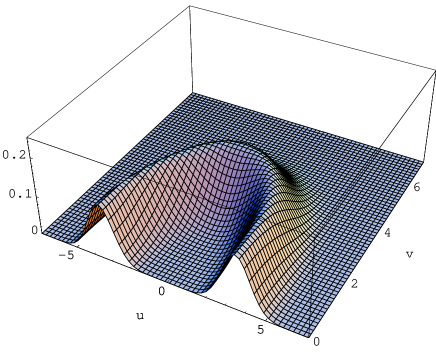
Figure 1: $\gamma=2$ case: Left, the square of the wave packet $|\psi(u,v)|^{2}$ for $\omega^{2}=1$, $\beta=1$, $\chi=3.5$ and $N=15$. Right, the contour plot of the same figure with the classical path superimposed as the thick solid line.

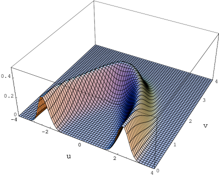
Figure 2: $\gamma=4$ case: Left, the square of the wave packet $|\psi(u,v)|^{2}$ for $\omega^{2}=1$, $\beta=1$, $\chi=4$ and $N=15$. Right, the contour plot of the same figure with the classical path superimposed as the thick solid line.

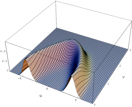
Figure 3: $\gamma=6$ case: Left, the square of the wave packet $|\psi(u,v)|^{2}$ for $\omega^{2}=1$, $\beta=1$, $\chi=3$ and $N=15$. Right, the contour plot of the same figure with the classical path superimposed as the thick solid line.

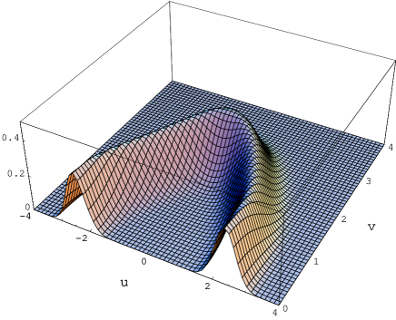
Figure 4: $\gamma=4$ case: Left, the square of the wave packet $|\psi(u,v)|^{2}$ for $\omega^{2}=-1$, $\beta=1$, $\chi=4$ and $N=15$. Right, the contour plot of the same figure with the classical path superimposed as the thick solid line.

4 Causal interpretation

To make the connection between the classical and quantum results more concrete, we can use de Broglie-Bohm interpretation of quantum mechanics. In this interpretation the wave function is written as

$$\Psi(u,v)=R\,e^{iS},$$ (49)

where $R=R(u,v)$ and $S=S(u,v)$ are real functions and satisfy the following equations

$$\left(\frac{\partial S}{\partial u}\right)^{2}+\omega_{1}^{2}u^{2}-\frac{1}{R}\frac{\partial^{2}R}{\partial u^{2}}-\left(\frac{\partial S}{\partial v}\right)^{2}-\omega_{2}^{2}v^{2}+\frac{1}{R}\frac{\partial^{2}R}{\partial v^{2}}+\frac{9}{4}\beta(u^{2}-v^{2})^{(\gamma+1)/3} = 0,$$ (50)

$$R\frac{\partial^{2}S}{\partial u^{2}}-R\frac{\partial^{2}S}{\partial v^{2}}+2\frac{\partial R}{\partial u}\frac{\partial S}{\partial u}-2\frac{\partial R}{\partial v}\frac{\partial S}{\partial v} = 0.$$ (51)

To write $R$ and $S$, it is more appropriate to separate the real and imaginary parts of the wave packet

$$\Psi(u,v)=x(u,v)+iy(u,v),$$ (52)

where $x,y$ are real functions of $u$ and $v$. Using (49) we have

$$R = \sqrt{x^{2}+y^{2}},$$ (53)

$$S = \arctan(\frac{y}{x}).$$ (54)

On the other hand, the Bohmian trajectories are governed by

$$p_{u}=\frac{\partial S}{\partial u},$$ (55)

$$p_{v}=\frac{\partial S}{\partial v},$$ (56)

where $p_{u}$ and $p_{v}$ are the momenta conjugate to $u$ and $v$ variables, respectively. Therefore, the Hamiltonian constraint ($H=0$) is again satisfied, but in the presence of the modified potential (50). The Bohmian equations of motion take the form

$$\dot{u}=\frac{1}{2}\frac{1}{1+\left(\frac{y}{x}\right)^{2}}\frac{d}{du}\left(\frac{y}{x}\right),$$ (57)

$$\dot{v}=-\frac{1}{2}\frac{1}{1+\left(\frac{y}{x}\right)^{2}}\frac{d}{dv}\left(\frac{y}{x}\right),$$ (58)

where $x$ and $y$ are known functions of $u$ and $v$ (41). These differential equations can be solved numerically to find the time evolution of $u$ and $v$.

Using the explicit form of the wave packets, these differential equations can be solved numerically to find the time evolution of $u$ and $v$. First, consider the case when $\gamma=2$. In this cases, it is apparent that the full potential for $u$ ($v$) is no longer equal to $u^{2}$ ($v^{2}$) but is $u^{2}-\frac{1}{R}\frac{\partial^{2}R}{\partial u^{2}}$ ($v^{2}-\frac{1}{R}\frac{\partial^{2}R}{\partial v^{2}}$). In the right part of figures 5 and 6, we have shown the classical and Bohmian trajectories together for two different choices of initial wave function ($A(n)=\frac{\,\chi^{n}}{\,{\sqrt{2^{n}\,n!}}}e^{-\chi^{2}/4}$, $A(n)=\frac{n\,\chi^{n}}{\,{\sqrt{2^{n}\,n!}}}e^{-\chi^{2}/4}$). We see that the Bohmian trajectories are in good agreement with the classical counterparts. Now, let us find the quantum potential for instance in $u$ direction along the Bohmian trajectories which is given by

$$V_{Q}=-\frac{1}{R}\frac{\partial^{2}R}{\partial u^{2}}=-\frac{x^{\prime 2}+x\,x^{\prime\prime}+{y^{\prime}}^{2}+y\,y^{\prime\prime}}{{x}^{2}+{y}^{2}}+\left(\frac{x\,x^{\prime}+y\,y^{\prime}}{{x}^{2}+{y}^{2}}\right)^{2}$$ (59)

where prime denotes the derivative with respect to $u$. Figure 7 shows the classical ($V_{C}$) and quantum ($V_{Q}$) potentials for two mentioned initial conditions. In particular, for $A(n)=\frac{\,\chi^{n}}{\,{\sqrt{2^{n}\,n!}}}e^{-\chi^{2}/4}$, we found that for $\chi\gtrsim 3$ (where $\chi$ is also the classical radius of motion for this choice of expansion coefficients) the functional form of the quantum potential is $V_{Q}=V_{Q}(x/\chi)$ with the maximum value at $x=\chi$. This means that

$$\frac{V_{Q}^{\mbox{\footnotesize max}}}{V_{C}^{\mbox{\footnotesize max}}}\propto\frac{1}{\chi^{2}},\hskip 28.45274pt\mbox{for}\hskip 28.45274pt\chi\gtrsim 3.$$ (60)

Moreover, as indicated in Fig. 8, initial Bohmian velocity coincides well with the classical counterpart for large $\chi$ which is compatible with the smallness of the quantum potential (60). In fact, for this choice of expansion coefficients, the initial wave function consists of two lumps centered at $u=\pm\chi$ as (Fig. 9)

$$\psi(u,0)=\frac{1}{2\pi^{1/4}}\left(e^{-(u-\chi)^{2}/2}+e^{-(u+\chi)^{2}/2}\right).$$ (61)

Therefore, the complete classical and quantum correspondence occurs when there is no significant overlap between the two pieces of $\psi(u,0)$. This means that to have a good correspondence for small radii, we need to choose a different set of coefficients or initial wave function which leads to a more localized wave function with infinitesimal overlap between its parts. We can also use causal interpretation for other cases. In particular, Fig. 10 shows the obtained Bohmian positions versus time (i.e. $u(t)$) for $\gamma=4$ and $\gamma=6$ which coincide well with their classical counterparts.

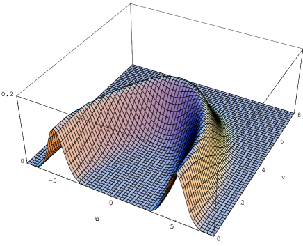
Figure 5: $\gamma=2$ case: Left, the square of the wave packet $|\psi(u,v)|^{2}$ for $A(n)=\frac{\,\chi^{n}}{\,{\sqrt{2^{n}\,n!}}}e^{-\chi^{2}/4}$ and $\chi=5$. Right, the classical (dashed line) and Bohmian (solid line) trajectories.

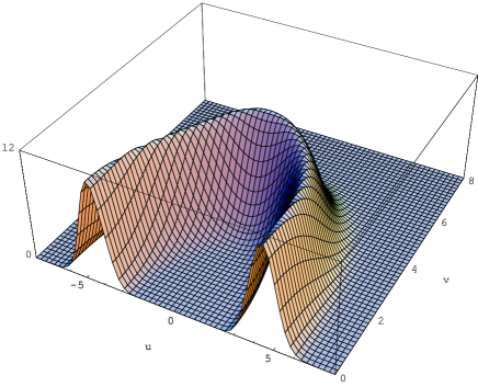
Figure 6: $\gamma=2$ case: Left, the square of the wave packet $|\psi(u,v)|^{2}$ for $A(n)=\frac{n\,\chi^{n}}{\,{\sqrt{2^{n}\,n!}}}e^{-\chi^{2}/4}$ and $\chi=4$. Right, the classical (dashed line) and Bohmian (solid line) trajectories.

Figure 7: $f_{1}(u,v)$: Classical (solid line) and quantum mechanical (dashed line) potentials for two types of initial conditions: Left, $A(n)=\frac{\chi^{n}}{\,{\sqrt{2^{n}\,n!}}}e^{-\chi^{2}/4}$ and $\chi=5$; Right, $A(n)=\frac{n\,\chi^{n}}{\,{\sqrt{2^{n}\,n!}}}e^{-\chi^{2}/4}$ and $\chi=4$.

Figure 8: $\gamma=2$ case: Classical (dashed line) and Bohmian (solid line) initial velocity versus $\chi$ for $A(n)=\frac{\chi^{n}}{\,{\sqrt{2^{n}\,n!}}}e^{-\chi^{2}/4}$.

Figure 9: $\gamma=2$ case: Left, the initial wave function $\psi(u,0)$ and right, the initial slope of the wave function $i\psi^{\prime}(u,0)$ for $A(n)=\frac{\,\chi^{n}}{\,{\sqrt{2^{n}\,n!}}}e^{-\chi^{2}/4}$ and $\chi=3.5$.

Figure 10: Classical and Bohmian values of $u$ versus $t$ for $\gamma=4$ (left) and $\gamma=6$ (right) with the initial conditions of Figs. (3,4), respectively.

5 Conclusions

We have described a Stephani type cosmology near its symmetry center leading to classical dynamical equations given by (22-24) and the corresponding WDW equation represented by (25). All these equations are not exactly solvable and we have solved these equations numerically by an implementation of the SM for the quantum cosmology cases. We then constructed the wave packets via canonical proposal which exhibit a good classical-quantum correspondence. This method proposes a particular connection between position and momentum distributions which correspond to their classical quantities and respect to the uncertainty principle at the same time. Here, using canonical prescription, we tried to construct the wave packets which peak around the classical trajectories and simulate their classical counterparts. We have also studied the situation using de-Broglie Bohm interpretation of quantum mechanics to quantify our purpose of classical and quantum correspondence and showed that the Bohmian positions and momenta coincide well with their classical values upon choosing arbitrary but appropriate initial conditions. Moreover, We showed that, in some cases, contrary to FRW cases, the bound state solutions also exist for all positive values of the cosmological constant.

References

- [1] G. Riess, et al, Astron. J. 116, 1009 (1998).
- [2] A. Vilenkin, Phys. Rev. Lett. 53, 1016 (1984).
- [3] R. L. Davies, Phys. Rev. D 36, 997 (1997).
- [4] V. Silveira and I. Waga, Phys. Rev. D 50, 4890 (1994).
- [5] M. Kamionkowski and N. Toumbas, Phys. Rev. Lett. 77, 587 (1996).
- [6] R. R. Caldwell, D. Rahul and P. J. Steinhardt, Phys. Rev. Lett. 80, 1582 (1998).
- [7] P. Pedram, S. Jalalzadeh and S. S. Gousheh, Int. J. Theor. Phys 46 3201 (2007), arXiv:0705.3587.
- [8] D. Kramer, H. Stephani, M. A. H. MacCallum, E. Herlt, Exact solutions of Einstein’s field equations,(Cambridge University Press, Cambridge, U.K, 1980).
- [9] A. Krasiński, Inhomogeneous Cosmological Models, (Cambridge University Press, Cambridge, U.K, 1998).
- [10] H. Stephani, Commun. Math. Phys. 4, 137 (1967).
- [11] A. Barnes, Gen. Rel. Gravit. 2, 147 (1974).
- [12] A. Krasiński, Gen. Rel. Grav. 15, 673 (1983).
- [13] P. Pedram, S. Jalalzadeh and S. S. Gousheh, Phys. Lett. B 655, 91 (2007), arXiv:0708.4143.
- [14] P. Pedram, S. Jalalzadeh and S. S. Gousheh, Class. Quantum Grav. 24, 5515 (2007), arXiv:0709.1620.
- [15] B. F. Schutz, Phys. Rev. D 2, 2762 (1970).
- [16] B. F. Schutz, Phys. Rev. D 4, 3559 (1971).
- [17] B. S. DeWitt, Phys. Rev. 160, 1113 (1967).
-
[18]
C. Kiefer, Nucl. Phys. B 341, 273 (1990);
C. Kiefer, Phys. Rev. D 38, 1761 (1988);
C. Kiefer, Phys. Lett. B 225, 227 (1989). - [19] T. Dereli, M. Onder and R. W. Tucker, Class. Quantum Grav. 10, 1425 (1993).
- [20] F. Darabi and H. R. Sepangi, Class. Quantum Grav. 16, 1565 (1999).
- [21] S. S. Gousheh and H. R. Sepangi, Phys. Lett. A 272, 304 (2000).
- [22] S. S. Goushe, H. R. Sepangi, P. Pedram, and M. Mirzaei, Class. Quantum Grav. 24, 4377 (2007).
- [23] P. Pedram, S. Jalalzadeh, Phys. Lett. B, 660, 1 (2008), arXiv: 0712.2593.
- [24] P. Pedram, M. Mirzaei and S. S. Gousheh, Computer Physics Communications, 176, 581 (2007).
- [25] R. Arnowitt, S. Deser and C. W. Misner, Gravitation: An Introduction to Current Research, edited by L. Witten, Wiley, New York (1962).
- [26] H. Stephani, Commun. Math. Phys. 5, 337 (1967).
- [27] M. P. Da̧browski, J. Math. Phys. 34, 1447 (1993).
- [28] M. P. Da̧browski, Astrophys. J. 447, 43 (1995).
- [29] J. Stelmach and I. Jakacka, Class. Quantum Grav. 18, 2643 (2001).
- [30] W. Godlowski, J. Stelmach, M. Szydlowski, Class. Quant. Grav. 21, 3953 (2004), arXiv:astro-ph/0403534.
- [31] R. A. Sussman, Gen. Rel. Grav. 32, 1527 (2000).
- [32] N. Deruelle, D. S. Goldwirth, Phys. Rev. D 51, 1563 (1995).
- [33] J. Ibáñez, I. Olasagasti, J. Math. Phys. 37, 6283 (1996).
- [34] S. E. Perez Bergliaffa, K. E. Hibberd, Int. J. Mod. Phys. D 8, 705 (1999).
- [35] F. Darabi, Phys. Lett. A 259, 97 (1999).
- [36] F. Darabi, A. Rastkar, Gen. Rel. Grav. 38, 1355 (2006).
- [37] S. Jalalzadeh, F. Ahmadi, H. R. Sepangi, JHEP 0308, 012 (2003).
- [38] J. P. Boyd, Chebyshev & Fourier Spectral Methods, Springer-Verlag, BerlinHeidelberg, (1989).