Absolute Physical Calibration in the Infrared

Abstract

We determine an absolute calibration for the MIPS 24$\mu$m band and recommend adjustments to the published calibrations for 2MASS, IRAC, and IRAS photometry to put them on the same scale. We show that consistent results are obtained by basing the calibration on either an average A0V star spectral energy distribution (SED), or by using the absolutely calibrated SED of the sun in comparison with solar-type stellar photometry (the solar analog method). After the rejection of a small number of stars with anomalous SEDs (or bad measurements), upper limits of $\sim$ 1.5% (rms) are placed on the intrinsic infrared SED variations in both A dwarf and solar-type stars. These types of stars are therefore suitable as general-purpose standard stars in the infrared. We provide absolutely calibrated SEDs for a standard zero magnitude A star and for the sun to allow extending this work to any other infrared photometric system. They allow the recommended calibration to be applied from 1 to 25$\mu$m with an accuracy of $\sim$ 2%, and with even higher accuracy at specific wavelengths such as 2.2, 10.6, and 24$\mu$m, near which there are direct measurements. However, we confirm earlier indications that Vega does not behave as a typical A0V star between the visible and the infrared, making it problematic as the defining star for photometric systems. The integration of measurements of the sun with those of solar-type stars also provides an accurate estimate of the solar SED from 1 through 30$\mu$m, which we show agrees with theoretical models.

1 Introduction

For many applications of astronomical photometry, an accurate absolute calibration in physical units and at multiple wavelengths is critical. Previous calibrations have made use of two basic approaches (Rieke et al. 1985). In direct calibrations, measurements are made of celestial sources in ways allowing the signals to be compared directly (if sometimes through a long chain of measurements) with signals from calibrated emitters. For indirect calibrations, direct calibrations at wavelengths well removed from those of interest are interpolated or extrapolated through physical modeling of astronomical sources. For direct calibrations, rigorous error analysis is possible, although there is always a risk of systematic terms that are not captured. Error analysis is far more difficult for indirect calibrations, since the systematic errors in theoretical modeling are often not apparent and there is usually no rigorous way to quantify the errors. Therefore, indirect calibrations must be used with caution until they have been confirmed by other indirect approaches or, better, by direct ones.

Infrared calibrations have often included some aspect of indirect calibration by extrapolating from the high quality visible direct calibrations. There are now high quality direct calibrations in the infrared, so the extrapolations can be tested. In this work, we start with the infrared calibrations, test their internal consistency, and then examine the consequences for extrapolation from them into the visible. This approach is preferred in principle because stellar behavior is relatively simple in the infrared (e.g., small temperature uncertainties have little effect on the shape of a nearly Rayleigh-Jeans spectrum for stars of the temperatures considered here).

The 24$\mu$m band of the Multiband Imaging Photometer for Spitzer (MIPS) achieves high photometric accuracy - with typical errors an order of magnitude smaller than those previously achieved at similar wavelengths (Rieke et al. 2004; Engelbracht et al. 2007). The Infrared Array Camera (IRAC) also is providing a large body of accurate and homogeneous photometry in the 3 - 8$\mu$m range (Fazio et al. 2004; Reach et al. 2005). In addition, a new absolute calibration of unprecedented accuracy is now available in the thermal infrared (Price et al. 2004). These advances make it both desirable and feasible to establish a very accurate calibration of the MIPS photometry at this wavelength and to provide guidelines to tie it in consistently with photometry at shorter wavelengths.

Bessell (2005) has reviewed photometry in general, but with only a few comments on the infrared. Price (2004) has reviewed infrared calibrations. His review concentrates on a huge body of work by Cohen, Walker, Witteborn, Price, and other co-workers on this topic. The review states that the results are ”in substantial disagreement with previous direct calibrations,” thus leaving open the question of possible undetected systematic errors. In addition, the review points out a number of discrepancies between the measured properties of the sun (e.g., Thuillier et al. 2003) and measurements of solar analog stars, which indicate possible issues in the photometric system.

The availability of large and homogeneous sets of data such as the Hipparcos photometric catalog (Perryman et al. 1997) and the 2MASS survey (Cutri et al. 2003) opens new possibilities to probe these issues and to improve calibrations, as well as providing a solid foundation to extend calibrations uniformly over the entire sky. Doing so is the goal of this paper. The paper is organized as follows. In Section 2, we review measurements of the absolute flux from Vega at 2.22 and 10.6$\mu$m, and the extrapolation of these measurements to the MIPS effective wavelength of 23.675$\mu$m. In Section 3, we discuss an independent approach to calibration using the solar analog method introduced by Harold Johnson (1965a). In Section 4, we show explicitly the discrepancy in the Vega-based visible calibration and the infrared one. In Section 5, we recommend adjustments to the absolute calibration of other photometric systems to bring them into agreement with the work reported here. The paper is summarized in Section 6. Those not wishing to plow through the details can go to that section for a summary of the useful results, which include recommendations for an absolute calibration accurate to 2% or better across the near and mid infrared.

2 Direct Infrared Calibrations of ”Vega”

2.1 Zero Point

Traditionally, absolute calibration systems have been referred to a ”zero point” of a magnitude system, usually defined by the spectral energy distributions of A stars. The Johnson/Arizona system defined the zero point as an average of the colors of a number of A stars, not just those of Vega, and as a result the magnitude of Vega is slightly positive ($\sim$ 0.02) at most bands. This situation has caused confusion because some have used Vega by itself to define zero magnitude, introducing a small offset in nominally similar systems. Further complications arise for the wavelengths of interest for this paper because of the contribution of the Vega debris system to the fluxes from this star beyond 10$\mu$m (e.g., Aumann et al. 1984). In addition, Vega is a rapidly rotating pole-on star with a significant temperature gradient ($\sim$ 1500K) from its pole to its equator (Gulliver et al. 1994; Aufdenberg et al. 2006), so its spectral energy distribution (SED) can differ from conventional models that assume a non-rotating star with a single surface temperature.

Nonetheless, there is a large body of data based on Vega. Fortunately, in the infrared the differences in photospheric colors due to the rapid rotation and other modeling uncertainties are small (see Price 2004, Figure 5 and Section 4 below). We therefore quote the results relative to the flux density of ”Vega”, a mythical star with a spectral energy distribution given by a Kurucz 1993 model spectrum of an A0 star (Kurucz 2005) with T_eff = 9550, log g = 3.95, log z = -0.5, and normalized to measurements of Vega that are corrected, if necessary, for the infrared excess from the debris disk around this star. This convention maintains continuity with the large existing body of infrared photometry. We have compared this model with the 2003 version (Kurucz 2005); the differences at photometric resolution and at wavelengths longer than 1$\mu$m are less than 0.1%, while the V - K color is 0.2% bluer with the newer model, again a negligible difference for our purposes. Thus, the Kurucz Vega models provide a stable reference baseline in the infrared. We provide the specific model we have used in electronic form so it can be utilized explicitly in future work or in adjustments to the calibration (Appendix A). In the following, we place ”Vega” in quotes because the zero point of the system is defined by an idealized version of this star.

2.2 Mid-Infrared

In this subsection, we discuss absolute calibrations near 10$\mu$m and use them to establish a ”best” value of 35.03 $\pm$ 0.30 Jy for the monochromatic flux density of ”Vega” at 10.6$\mu$m. We also show that the absolute measurements at 21$\mu$m are consistent with this value and derive a monochromatic flux density for ”Vega” at the effective or mean wavelength of the MIPS 24$\mu$m band.

For reasons given in the introduction, we place highest weight on direct calibrations in the thermal infrared. Such measurements are summarized in Table 1. The two most accurate sets of measurements - Rieke et al. (1985) and Midcourse Space Experiment (MSX) - have estimated errors of 3% (Rieke et al. 1985) or $\sim$ 0.6% (Price et al. 2004) near 10$\mu$m and are in excellent agreement to within these errors. Rieke et al. (1985) review previous work (Becklin et al. 1973; Low and Rieke 1974) and show it agrees closely with their calibration, well within the errors of order 7% quoted for the earlier work. The solar analog calibration in this work agrees to within $\sim$1.5%, as does another calibration conducted in support of the Infrared Space Observatory (ISO) (both to be discussed below). The consistency of these independent determinations indicates that there are no major systematic errors. At 21$\mu$m, the agreement between the MSX calibration and previous work is also excellent although the errors estimated for the Rieke et al. (1985) measurements are about 7%. Even though Rieke et al. reported a direct measurement at this wavelength, they based the recommended calibration on an extrapolation from the 10.6$\mu$m calibration because they felt it was more accurate.

To obtain the best possible calibration in the mid-infrared, we therefore need an optimum way to combine the measurement of Rieke et al. (1985), the three near 10$\mu$m from Price et al. (2004), and the solar analog determination from this work. We do so at a wavelength of 10.6$\mu$m, using the ”Vega” spectral energy distribution as the means to interpolate or extrapolate to the same wavelength and thus to relate the measurements to each other. That is, the calibration is relative to the normalization in Price (2004), Figure 5. However, this figure plots the calibration of Rieke et al. (1985) incorrectly. The figure shows the proposed zero point of the photometric system as if Vega were zero magnitude but Rieke et al. (1985) set Vega to a magnitude of 0.02. That is, the measurement of Vega should be 0.02 lower than plotted, and hence in even better agreement with the MSX values than indicated (Price, private communication).

Various ways to combine the data are indicated in Table 1. For extrapolating to other wavelengths, we define the ”monochromatic” flux density to be proportional to the average over a 1% spectral bandwidth of $\nu^{-2}$ f_ν = $\lambda^{4}$ f_λ. For example, we determine the MSX value starting from the N band flux density in Tables 1 and 2 of Cohen et al. (1992), extrapolated to 10.6$\mu$m according to the ”Vega” SED. We used the standard deviation of the biases in bands A, C, and D in Table 9 of Price et al. (2004) to estimate a 1.1% rms scatter and then combined this value with the quoted uncertainties to compute a weighted average of the biases, which was used to adjust the Cohen et al. value for the flux density.

In the following section, we use the Rieke et al. and MSX weighted average as the basis to project the 10.6$\mu$m calibration back to 2.22$\mu$m, for comparison with direct measurements there. In Section 3.3.3, we use the direct calibration at 2.22$\mu$m, the IRAC 8$\mu$m measurements of solar-type stars, and the spectral energy distribution of the sun to obtain the independent new calibration listed as solar analog (this work).

We also tabulate the calibration of Hammersley et al. (1998), conducted in support of the ISO mission. They used the 1993 Kurucz model of Vega to extrapolate from K-band measurements, and quoted a photospheric flux density from this model at 10.47$\mu$m. We have corrected their value to 10.6$\mu$m and reduced it by 1.29% to correct for the K-band excess of Vega (Absil et al. 2006). It then agrees excellently with the other determinations. Hammersley et al. show that their measurements of stars within this system are also in close agreement with previous measurements of the same stars. We have not included this calibration in our average because it is not clear how to evaluate the errors, but they would appear to be similar to those of most of the other entries.

All of the approaches are consistent with the adopted value of 35.03 Jy for the monochromatic flux density of ”Vega” at 10.6$\mu$m. We quote a slightly increased error from the pure weighted average value to allow for any residual systematic errors. A measure of the degree of agreement is that the calibration ignoring the MSX result is accurate to 2% and agrees with the MSX calibration to within 1%.

We can now compute that the corresponding ”Vega” flux density at 23.675$\mu$m (the mean wavelength of the MIPS band) is 7.15 $\pm$ 0.11 Jy, where we have assigned a 1.5% error to allow for any issue in propagating the calibration to 24$\mu$m. MSX also obtained a calibration at 21.3$\mu$m, which is equivalent to a ”Vega” flux density at 23.675$\mu$m of 7.19 $\pm$ 0.11 Jy, i.e., is fully consistent with our extrapolation from 10.6$\mu$m. We take the average value of 7.17 $\pm$ 0.11 Jy = 3.835 X 10^-18 W cm^-2 $\mu$m^-1 as the ”best” estimate; we have not decreased the error bar in the average because the two determinations are not completely independent.

2.3 Near Infrared

This subsection addresses tying the absolute measurement at 10.6$\mu$m to direct calibrations of Vega near 2$\mu$m. Since the high-weight calibrations are at 2.20 and 2.25$\mu$m (Blackwell et al. 1983; Selby et al. 1983; Booth et al. 1989), we correct all of them to 2.22$\mu$m; this wavelength has the further advantage that it is well-removed from strong spectral absorptions in both A and G stars. Figure 5 of Price (2004) demonstrates that the predictions of A-star models are very similar in spectral shape between 2 and 24$\mu$m, and we obtain a similar result comparing the 1993 and 2003 Kurucz models for Vega. At shorter wavelengths, there can be slight deviations of models. However, the comparison of calibrations at 2 and 10$\mu$m and interpolations within this range should be robust.

The flux density from ”Vega” at 2.22$\mu$m is predicted to be 649 Jy, using the Kurucz model normalized at 10.6$\mu$m to the ”Rieke plus MSX” value. We assign a 1.5% error to this estimate to include any issues in propagating it from 10.6$\mu$m. This value is compared with the direct measurements of Vega by Walker (1969), Selby et al. (1983), Blackwell et al. (1983), and Booth et al. (1989) in Table 2. This list of measurements represents all the absolute calibrations in the literature except those based in some way on extrapolating the Vega spectrum (or, in the case of Campins et al. (1985) that are revised in this work). All the reported measurements in this table have been corrected to a wavelength of 2.22$\mu$m according to the Kurucz model spectrum of Vega.

Absil et al. (2006) report interferometric measurements of Vega at 2$\mu$m that show it has an excess of 1.29% $\pm$ 0.19% within a field of diameter 2”, presumably due to a hot inner circumstellar disk (see also Ciardi et al. 2001). We have corrected the direct measurements downward by 1.29% to remove the effects of this disk. It is unlikely that the output of the disk exceeds this value significantly. For example, the excess of $\sim$ 4% observed by MSX in bands C and D at 12.1 and 14.7$\mu$m (Price et al. 2004, Table 4) and an upper limit to the color temperature for the excess of 2000K (compare Absil et al. (2006)) predict an excess above the photosphere of 0.9% at 2.2$\mu$m. This rough upper limit is very close to the measured excess at this wavelength, i.e., there is no missing flux that might lie outside the 2” field. Although there are accurate direct measurements of the flux from Vega at other infrared wavelengths (e.g., Mountain et al. 1985), the lack of detailed understanding of the behavior of the circumstellar material makes it problematic to interpret these measurements to the level of accuracy that can be achieved at 2$\mu$m.

Nonetheless, because the extent and other aspects of the correction may be more uncertain than indicated by the nominal error bar, we have assigned an error of one percentage point to the correction. The resulting value is 645 $\pm$ 15 Jy for the directly measured flux density from the Vega photosphere at 2.22$\mu$m. The agreement with the value extrapolated from 10.6$\mu$m is virtually perfect. We combine the two values to determine a ”best” calibration.

The central result from this section is captured in Tables 1 and 2. The theoretical spectral energy distribution of ”Vega” links the accurate absolute measurements of this pseudo-star at 2.22 and 10.6$\mu$m well. Because consistent values are obtained in distinct calibrations with completely different chains of measurements and assumptions, this agreement appears not to be undermined by any plausible systematic errors. The uncertainties in our final derived flux densities for this ”star” are less than 1.5% at both wavelengths.

3 An Independent Verification via the Solar Analog Method

3.1 Spectral Energy Distribution of the Sun

A further test of the ”Vega”-based calibration is to show that an approach based on a different stellar type is consistent with it. To generate this new calibration, we use the solar analog method (Johnson 1965a). That is, we take the absolutely calibrated measurements of the sun and apply them as colors to other solar-type stars. This subsection discusses the various forms of solar SED that we examined.

3.1.1 Measurements of the Solar SED

We take the solar SED for 0.2 to 2.4$\mu$m from Thuillier et al. (2003 and private communication). This work supplants previous work, although it is generally consistent with the earlier measurements as summarized by Labs and Neckel (1968, 1970), to within a few percent.

Vernazza et al. (1976; hereafter VAL) provide a careful, critical assessment of the measurements at longer wavelengths. It is concluded that the data out to 12$\mu$m are of high quality. Specifically, Saiedy and Goody (1959) estimate that their measurement at 11.1$\mu$m is accurate to 0.7%, standard error. Saiedy (1960) estimates the standard errors at 8.63 and 12.02$\mu$m to be 0.9 and 1.8% respectively. Beyond that wavelength, the measurement accuracy decreases substantially. VAL made adjustments of $\sim$4% in some measurements to improve the apparent agreement. The quoted errors are also a few percent.

VAL described these results with a semi-empirical model . The model and the final adjusted set of measurements from VAL are described well by a functional fit due to Engelke (1992), which we will use to represent the long wavelength observations for the rest of this paper. We assign a 5% uncertainty to the measurements beyond 12$\mu$m as represented by the Engelke (1992) function.

3.1.2 Models of the Solar SED

We have compared the measurements with two photospheric models that predict the solar spectral energy distribution. They are described in more detail here.

The model of Holweger & Müller (1974, hereafter HM74) is based on a local thermal equilibrium (LTE) analysis of solar line observations. The thermal structure of the temperature minimum region and the chromosphere lying above the photosphere is controversial. The solar temperature structure appears to have a minimum of $\sim$ 4000K near a depth of 500km in the photosphere, with an overlying 1500km thick, 7000K plateau in the mechanically heated chromosphere. However, the analysis of carbon monoxide (CO) lines indicates a very cool brightness temperature ($\sim$ 3700K) at the extreme edge of the solar disk, where the slanted line of sight probes into the low chromosphere (see Ayres et al. 2006). In a study of the CO fundamental lines, Harris et al. (1987) concluded that the HM74 photospheric model was consistent with the visible continuum center-limb behavior and the properties of the CO fundamental spectrum. Using visible continuum intensities and center-limb behavior in combination with the CO center-limb behavior, Ayres et al. (2006) recently re-determined the solar photospheric thermal profile, which also closely resembles the HM74-model structure.

Theoretical IR spectra were calculated using the HM74 model and the TurboSpectrum program described by Plez et al. (1993), and further updated. The program treats the chemical equilibrium for hundreds of molecules with a consistent set of partition functions and dissociation energies. Solar abundances from Anders & Grevesse (1989) have been assumed, except for the iron abundance, $\varepsilon$(Fe) = 7.51, which is in better agreement with the meteoritic value. The continuous opacity sources considered are H^-, H, Fe, (H+H), H${}_{2}^{+}$, H${}_{2}^{-}$, He I, He I_ff, He^-, C I, C II, C I_ff, C II_ff, C^-, N I, N II, N^-, O I, O II, O^-, CO^-, H₂O^-, Mg I, Mg II, Al I, Al II, Si I, Si II, Ca I, Ca II, H₂(pr), He(pr), e${}^{-}_{sc}$, H${}^{-}_{sc}$, H${}_{2}\quad{}_{sc}$, where ‘pr’ stands for ‘pressure induced’ and ‘sc’ for ‘scattering’. The main continuous absorber in the IR is H${}^{-}_{ff}$, for which the absorption coefficients of Bell & Berrington (1987) were used. For the line opacity, we used the atomic and molecular database created by Decin (2000) and Decin et al. (2003). The main molecules included are CO, SiO, H₂O, OH, NH, CH, CN, and HF. A full spectrum from 2 to 200$\mu$m was generated at a resolution of $5\times 10^{-5}$ $\mu$m.

The Fontenla et al. (2006) model assumes a temperature minimum of 4500K and is computed only to a temperature of 5374K in the low chromosphere. It has been found that the higher chromospheric layers do not affect the spectrum between 1 and 100$\mu$m. The densities are computed from hydrostatic equilibrium and charge conservation, and the calculation assumes local thermal equilibrium (non-LTE effects have negligible influence on the infrared spectrum). Further details are given by Fontenla et al. (2006).

3.1.3 Synthetic Solar Colors

All of the approaches discussed above for describing the measurements or modeling the solar output agree excellently in the 2 to 4$\mu$m region. There are modest divergences at longer wavelengths (particularly beyond 10$\mu$m), but still generally within the expected errors.

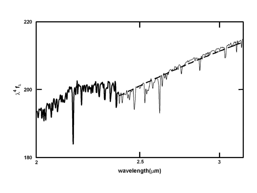
Figure 1: Joining the segments for a complete solar spectrum. The heavy line is the measured spectrum from Thuillier et al. (2003). The dashed heavy line is the Engelke approximation. Both of these curves are left in the measured units with no re-normalization. The light solid line is the modified HM74 model that we use to represent the empirical solar spectrum, normalized to provide a smooth transition from the Thuillier et al. spectrum consistent with the Engelke approximation.

We will therefore use photometry of solar-type stars to help decide among the possibilities. The first step is to compute synthetic colors for comparison with the stellar photometry. We use the Thuillier et al. (2003) solar spectrum at wavelengths short of 2.4$\mu$m and the Engelke function beyond 2.4$\mu$m to represent the measurements of the sun . They join in a consistent manner with no renormalization, as shown in Figure 1. Synthetic colors are also computed directly for the models. To compute the K-band signal for HM74, we continued the model to wavelengths short of 2$\mu$m based on the Thuillier et al. measurements. The exact form of this continuation has only a modest influence on the K photometric color.

In the following sections, we will use near infrared magnitudes as defined by the 2MASS system. To determine synthetic colors for the sun, we took the relative response functions from the 2MASS web site (originally from Cohen et al. 2003). The information on the IRAC 8$\mu$m band is from the IRAC Data Handbook. The MIPS 24$\mu$m relative spectral response is taken from the MIPS Data Handbook. We obtained the response of the V filter from Johnson (1965b) and multiplied it by a function proportional to wavelength to convert it into a relative response function. We convolved the Kurucz A star spectral energy distribution and the various models for the sun with these functions. The relative responses to the A-star and solar spectra can then be used to calculate the synthetic colors provided in Table 3.

3.2 Photometry of Solar-Type Stars

For comparison with the synthetic colors, we determine accurate averages for the measured stellar colors in this subsection. We emphasize the use of large sets of homogeneous measurements (Hipparcos, 2MASS, and homogeneous data sets with MIPS and IRAC). An essential aspect of these comparisons is the linearity of MIPS and IRAC over the range of the observations, which we demonstrate in Appendix B is adequate for our needs.

3.2.1 K_S - [8] Color of Solar-Type Stars and a Solar Analog Calibration

We first discuss our procedures at 8$\mu$m (further details are in Appendix C). The existing calibration of the IRAC photometry is relative to ”Vega” as the zero point, as described by Reach et al. (2005). We used their stated zero point to compare their assumed flux density for ”Vega” with ours. We first compute the monochromatic flux density at 7.872$\mu$m, and then apply their recommended color correction of 1.042. Extrapolating from the 2.22$\mu$m calibration we find a value 1.2% brighter than theirs, while extrapolating from 10.6$\mu$m we find one that is 1.7% brighter. Thus, to put their calibration on the same overall scale as is recommended here, an upward adjustment of about 1.5% is required.

We have used the Formation & Evolution of Planetary Systems (FEPS) Delivery 3 data products (NASA/IPAC Infrared Science Archive 2007) for a solar analog calibration at 8$\mu$m. We also need stars with very homogeneous near infrared photometry. We therefore required that each star have 2MASS measurements of ”A” quality in all three bands (JHK), and that they all be measured in the ”Read 1” mode (see Appendix D). In addition, we used the Hipparcos photometry at V to compute V - K colors and rejected any star departing by more than 0.10 magnitudes from the standard color. The final sample is listed in Table C1, and the IRAC reductions are described in Appendix C.

To look for intrinsic scatter in the stellar colors, we averaged the 2MASS J, H, and $K_{S}$ measurements to a single ”$SuperK_{S}$” value (see Appendix C). We have computed the ratio of 2.2$\mu$m to 8$\mu$m flux densities for the stars in Table C1, using the $SuperK_{S}$ magnitudes. We find that the rms scatter is only 2.05%. This value is smaller than would have been predicted from the combination of the uncertainties in the $SuperK_{S}$ magnitudes and in the IRAC 8$\mu$m flux densities. We conclude that the photometry is well behaved and that all of the stars have very similar SEDs between 2 and 8$\mu$m. (An exception arises at the CO fundamental and first overtone bands (bandheads at 4.6$\mu$m and 2.3$\mu$m respectively) due to variations in the absorption strength; these regions are not probed by the photometry we have used for calibration.)

Our empirical solar SED model (Thuillier plus Engelke) lies a factor of 1.026, or 0.028 magnitudes, above the ”Vega” SED, at 7.872$\mu$m, if they are set equal at 2.22$\mu$m. The average value of K_S - [8] from the measurements of the solar-type stars in Table C1 is a factor of 0.986 below the Thuillier/Engelke solar SED. The errors in the solar measurement should be small in this region, of order 1% (VAL). We can derive an independent calibration by normalizing to the results at 2.22$\mu$m based on the direct measurements of Vega in Table 2 (i.e., excluding the extrapolation from 10.6$\mu$m). The resultant calibration is entered in Table 1; we have assigned a 3% error, based on the error in the 2.22$\mu$m calibration and the uncertainties in propagating it to 10.6$\mu$m. It agrees well with the other calibrations.

We conclude that a completely independent check of the linkage of the 2.22 and 10.6$\mu$m calibrations via solar type stars agrees excellently with the results from direct absolute calibrations and the ”Vega” SED at both wavelengths.

3.2.2 Zero Color at 24$\mu$m

We now extend the solar analog method to 24$\mu$m, to test the various alternatives for the solar SED in this spectral region. We determine zero color at 24$\mu$m by averaging the measurements of a large number of A stars, similar in spirit to the original A-star-based zero point (Johnson and Morgan 1953). In our situation, the approach has a number of virtues. First, because it uses averages of many measurements, it achieves high accuracy in the comparison. Second, peculiar behavior by a few stars will have little influence on the results, and sufficiently peculiar stars stand out and can be rejected as outliers to make their influence disappear entirely. Third, the procedure removes our dependence on previous calibrations.

We selected the sample of stars to use at 24$\mu$m from Su et al. (2006) supplemented by stars in the MIPS calibration program. We eliminated all stars with indications of excess emission at either 24 or 70$\mu$m (Su et al. (2006) show that $\sim$ 32% of typical A stars have excess emission at 24$\mu$m). To guard against subtle excesses, we also eliminated stars younger than 200 Myr, since the excesses at 24$\mu$m decay roughly as time/150Myr (Rieke et al. 2005). The stars are listed along with their key parameters in Table C2 (Appendix C). Appendix C also describes our reduction procedures at 24$\mu$m in detail.

We have fitted a Gaussian to the distribution of $SuperK_{S}$ over 24$\mu$m flux density ratios (normalized to one) for our A star sample. The standard deviation is 0.048 (we have excluded HD 172728 from the fits because its low values for two measurements imply a possible problem with the 2MASS measurement and also the two stars with the highest ratios, HD 11413 and HD 92845, since they may have weak excess emission). By taking the quadratic difference of the fitted standard deviation and the estimated errors in the 24$\mu$m and $SuperK_{S}$ values, we find a residual uncertainty term of 3%. This value is an upper limit to the intrinsic star-to-star rms differences in K_S - [24] photospheric color.

Because the intrinsic scatter appears to be small, we assume that the scatter in the colors is dominated by measurement errors and it is appropriate to reduce the uncertainties by averaging. We found that attempting to correct the K_S measurements for extinction had a negligible effect on the average (0.004 magnitudes) and increased the scatter, so we have used the uncorrected K_S values. In an arbitrary normalization that brings the value of the flux density ratios close to 1 (and will be preserved for a similar calculation for solar type stars) the average ratio of K_S to 24$\mu$m flux densities is 0.964 $\pm$ 0.008.

3.2.3 24$\mu$m Measurements of Solar-Type Stars

We now apply the identical procedures to 24$\mu$m measurements of a suite of solar-type stars. Our sample is drawn largely from the FEPS program, Delivery 3 data products. It is listed in Table C3 and Appendix C gives the details of our reductions. To guard against excess emission, we have only included stars older than one Gyr as determined by Wright et al. (2004).

We computed $SuperK_{S}$ magnitudes for these stars (see Appendix C). A Gaussian fitted to the resulting distribution of $SuperK_{S}$ to 24$\mu$m flux ratios (normalized to 1) has a standard deviation of 0.034. A quadratic subtraction of the estimated measurement errors from the fitted standard deviation leaves less than 1% for the intrinsic scatter due to variations in the stellar SEDs.

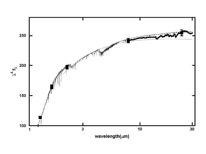
Figure 2: Infrared spectrum of the sun. The spectrum has been multiplied by $\lambda^{4}$ to facilitate detailed comparisons in the infrared. Out to 2.4$\mu$m, we plot the measured solar spectrum, based on the results of Thuillier et al. (2003). Beyond this wavelength, the solar spectrum is represented by the HM74 model, normalized and modified at the CO fundamental bands as described in the text. The photometry of solar type stars (normalized at V) is shown as square points, and we have put a 2% error bar on the measurement at 24$\mu$m. Between 8 and 32$\mu$m, we also show the spectrum of solar-type stars obtained with the Spitzer Infrared Spectrograph (black curve). The smooth curve below the spectrum is the Engelke (1992) approximation to the solar continuum.

For the calibration calculation, we reject the two lowest and two highest values. The average normalized ratio of $K_{S}$ to 24$\mu$m flux density is 1.005 $\pm$ 0.007. The ratio of the two averages for A and solar-type stars, 1.042, is then the color in flux units of a solar-type star relative to the A-star zero point. It is equivalent to a color in magnitudes of 0.045 $\pm$ 0.011 in the sense that the solar-type stars are redder than A0V stars. As shown in Table 3 and Figure 2, the resultant value for the sun at 24$\mu$m is 5% above the Engelke function, and we have assigned an error of 5% to this function at these wavelengths. Hence, the agreement is within the errors. However, the color of the solar-type stars is well enough determined to suggest that the Engelke function is 3 to 7% too blue relative to the true solar SED.

3.2.4 Solar Analog Calibration at V, J, H, and K

We can test the V, J, H, and K-band calibration by checking to see if we get the correct colors for the sun. From the synthetic colors, we find V - K_S = 1.568. The error is a combination of that in the K absolute calibration and in the measurements of the sun. ¿From Table 2, we take the first error category to be 1.2%. The second class of errors is quoted by Thuillier et al. (2003) as 1.1, 0.8, 0.65, and 0.6% 1-$\sigma$ respectively at 0.95, 1.5, 1.1, and 2.5$\mu$m. We therefore quote a net error of 2%. Similar errors should hold for the other bands.

In principle, this solar color should agree with the colors of similar stars. The V and K_S colors of Vega and solar analog stars are tied together by accurate direct calibrations. However, the J and H 2MASS measurements are determined by color transformation and interpolation of the direct calibrations. For 2MASS observations of these relatively bright stars, it is possible that there are residual errors at the 1 to 2% level. Therefore, rather than assuming the 2MASS color zero points, we determined the zero points for the J and H bands by averaging measurements of a large number of A0V stars also measured in the Read 1 mode. Our procedure is discussed in Appendix D. We then corrected the catalog solar analog colors to these zero points.

Our sample of solar-type stars is largely from the NStars compilation (Gray 2007). We fitted the trend of colors with temperature and used the fit to adjust them all to match the color expected for a star with a temperature of 5778K (the effective temperature of the sun) - see Appendix D. The final average V - K_S color of 1.545 $\pm$ 0.015 is compared with the V - K_S of the sun in Table 3.

Our value of $<$V - K_S$>$ = 1.545 for the average of solar-type stars differs substantially from standard tabulations such as 1.46 in Tokunaga (2000), as well as other determinations such as that of Holmberg et al. (2006). Part of these discrepancies may be traceable to the 0.045 magnitude correction implied for the SED anomalies of Vega, but another important contributor is possible discrepancies in translating the solar temperature into the stellar temperature scale (Holmberg et al. 2006). There is also significant scatter in assigned temperatures within a spectral type in the Nstars compilation (Gray 2007), equivalent to at least one spectral subtype. Roughly speaking, a shift of 10K in the temperature of a solar-type star shifts its V - K by 0.01.

For another comparison, we used a very carefully compiled and clearly described set of colors provided by Bessell et al. (1998): see Appendices A - C of their paper. They define a magnitude system in which V - K = 0 for Vega, and have forced the calibration to fit both this color definition and a similar model for ”Vega” as the one used in this paper. By forcing the ”Vega” model to fit the infrared calibrations, we find a system in which V - K = 0.045 for Vega the real star (see below). From Carpenter (2001), we find an additional adjustment of 0.018 from the Glass/SAAO system to 2MASS, or a total of 0.063. Table 4 allows comparison of the various estimates of V - K_S with the Bessell et al. (1998) results corrected to the same basis as ours. Details regarding the first four entries in this table can be found in Bessell et al. (1998). We have also entered the measurements from Table 3 to demonstrate the good agreement. We show additional synthetic colors from models computed by Casagrande et al. (2006). They assumed a $V-K_{S}$ color of 0.047 for Vega, bringing their scale close to the one we have used (with $V-K_{S}=0.045$). The prime solar-type NICMOS calibrator, P330E, can be used as an independent test of these colors. We show in Table 4 the colors of P330E relative to a synthetic V magnitude (Bohlin et al. 2001). We have interpolated to provide a K_S magnitude. All of these determinations of the solar $V-K_{S}$ color agree very well.

We also computed J - K_S and H - K_S colors for the 32 solar-type stars listed in Table D2 with A grade Read 1 measurements in all three bands (this criterion eliminates HD 41330, 90508, 168009, and 186427 from the sample). Since these colors are relative to the 2MASS system, we corrected them for the slight deviations from zero color we found for A0 stars (see Appendix D). The average colors are listed in Table 3 and plotted in Figure 2 for comparison with the solar SED. The errors are estimates from those quoted in the 2MASS catalog, with some allowance for systematic effects. The agreement with the solar colors is excellent.

The infrared colors also agree well with those in Tokunaga (2000): H - K = 0.061 for us, vs. 0.05, and J - H = 0.326 vs. 0.32. We can also compare with Bessell et al. (1998), but we first transform the J - K_S to the Johnson/Glass system by subtracting 0.007 magnitudes, determined from the Thuillier solar SED. We then find J - K = 0.38 and H - K = 0.054, compared with J - K = 0.38 and H - K = 0.045 from their tabulation of the solar analog determinations of Cayrel de Strobel (1996).

If we predict errors from the quoted uncertainties in the 2MASS measurements, we obtain a predicted error for a typical J - K_S measurement of 3.1%, whereas the scatter in this color indicates a typical error of 2.3%. This behavior is consistent with some degree of correlation in the 2MASS measurements, which is reasonable. There is no indication of scatter in the intrinsic colors of the stars. A similar argument indicates no detected intrinsic scatter in H - K_S.

We have made a more demanding test for the uniformity of the JHK colors of solar-type stars. We used the accurate near infrared photometry of Kidger & Martín-Luis (2003), which for well-measured stars has errors of less than 1%. We did not use other available high accuracy photometry compilations that concentrate on faint sources to calibrate infrared arrays, since these stars are more distant and subject to reddening. We selected the 16 stars from Kidger & Martín-Luis with listed spectral types of G0 through G5 IV or V, with $1.4<V-K<1.8$, with six or more measurements, and with errors in all three bands indicated as $<$ 1%. We then fitted a straight line to the trends of $J-H$ and $H-K$ vs. $V-K$, finding scatter around the line of 1.5% in the first case and 0.9% in the second. We used $V-K$ instead of spectral type because we did not want the results to be subject to type errors. In addition, Kidger & Martín-Luis (2003) include a number of color-color plots that show small scatter that is independent of spectral type from A through K stars. We conclude that G stars have intrinsic scatter in the near infrared colors of no more than about 1%.

The ”anomalously red” color of the solar spectrum as measured by Thuillier et al. (2003) relative to such determinations as Holmberg et al. (2006) has not been satisfactorily explained previously (see discussion in Casagrande et al. 2006). It is comforting that, with care in analyzing the photometric database, we have found that this color is consistent with those of other solar-type stars, and that the scatter in color among such stars is small. As shown in Table 3, this color is consistent not only with the empirically measured solar colors but with the predictions of a large number of models of the solar SED.

3.2.5 Spectra

We have used the Spitzer Infrared Spectrograph (IRS) to confirm the slope and overall spectral behavior of the solar-type stellar SED between 8 and 30$\mu$m. The result, reduced as described in Appendix C, is plotted in Figure 2, normalized to the photometric point at 8$\mu$m. If it is normalized to the HM74 model at 8$\mu$m, the rms noise around the model continuum is $\sim$ 0.7%. It therefore confirms to high accuracy the overall shape of the SED of solar type stars as described by this model.

3.2.6 An Empirical Solar SED

As shown in Figure 2, the HM74 model agrees well with the measurements of both the sun and of solar-type stars: 1.) it tracks the Engelke function closely out to about 10$\mu$m; 2.) it is consistent with the solar-type stellar calibration at 8$\mu$m; 3.) it is also consistent with the solar-type stellar color at 24$\mu$m; and 4.) it agrees with the overall spectral shape of solar-type stars measured with IRS between 8 and 30$\mu$m. The model also includes a full treatment of the solar absorption line spectrum.

We therefore adopt it to describe the mid-infrared SED of the sun. To normalize it to the Thuillier et al. spectrum, we took advantage of the fact that the absolute level in the Engelke function agrees very closely with the Thuillier spectrum at 2.3 - 2.4$\mu$m, so we can use this fit as a smoothing function to help join the two spectra. Figure 1 illustrates how the HM74 model was joined to the Thuillier measurements.

The remaining issue is that the CO fundamental bands are difficult to fit a priori in models. We empirically adjusted the depth of these features by setting the CO absorption features to be consistent with the spectroscopy of Wallace & Livingston (2003). At their high spectral resolution, there are a number of atmospheric mini-windows that allow accurate measurement of CO equivalent widths. On average, we found that the HM74 model had slightly weaker CO absorption than found by Wallace & Livingston. We therefore used the Engelke approximation between 4 and 6.5$\mu$m as a featureless continuum, normalized to the HM74 model. We multiplied the Engelke SED by 0.125, subtracted it from the HM74 model, and renormalized the result to the original continuum level to bring the CO equivalent widths into agreement with those of Wallace & Livingston (2003). This modified spectrum was used to replace the HM74 values between 4 and 6.5$\mu$m.

Our final adopted solar spectrum is shown in Figure 2 and given numerically in Appendix A. The Engelke (1992) fit to the VAL model/reconciled measurements falls slightly below the empirical model at wavelengths longer than about 6$\mu$m. In the IRAC 8$\mu$m band, the discrepancy is 1.4%, at the outer limits of the errors. The model is therefore slightly discrepant with our calibration, based on accurate solar measurements. At 24$\mu$m, the model and the photometry differ from the solar measurements by 5%, but here the model result is to be preferred because of the larger errors in the solar measurements. In general, the model should represent the true solar SED to within $\sim$ 2%, an error estimated from a combination of the discrepancies with the solar measurements and the photometric errors in the solar-type stellar colors.

4 Vega at Wavelengths Short of 2$\mu$m

To extend these procedures to the visible range, we use the average of our ”best” calibrations at 10.6$\mu$m from Table 1 and at 2.22$\mu$m from Table 2 and the ”Vega” model to predict a value of 3714 Jy for Vega at 0.5556$\mu$m. Mégessier (1995) has summarized and reconciled various direct measurements of Vega, corrected to a wavelength of 0.5556$\mu$m. The preferred value for the reconciled measurements is 3563 Jy, 4.2% or 0.045 magnitudes less than we find at this same wavelength via the model. The net errors are only about 1% for the infrared and 0.7% at 0.5556$\mu$m. This value agrees with the results of Bohlin and Gilliland (2004), who find that the spectrum of Vega normalized at 0.5556$\mu$m and extrapolated using the 1993 Kurucz model to 2$\mu$m is 2% fainter than the calibration of Cohen et al. (2003), which we find in turn is 2% lower than our calibration. Thus, although the theoretical ”Vega” spectrum gives good agreement with measurements in the infrared, there is a significant discrepancy between the infrared and visible. This result is not new. Mégessier (1995) discusses it at length, summarizing many results that point to the same issue. As a result, this work considers the infrared calibration separately from the visible one for similar reasons as discussed here.

It seems likely that the departure from the model arises because Vega is a pole-on rapid rotator. With a measurement of the surface temperature distribution on the star (Aufdenberg et al. 2006), we can now address where its SED might depart sufficiently from the single-temperature models to be of concern for its use as a calibrator. The equatorial surface temperature is estimated to be 7900K, corresponding to type A7, which has V - K = 0.5, J - K = 0.09, and H - K = 0.03 (Tokunaga 2000). If we imagine the effective visible surface of the star to be a combination of A0 and A7 spectral type to give a net V - K = 0.045, by interpolation we expect an effect of $\sim$ 0.01 magnitudes in J - K and 0.003 magnitudes in H - K to allow for the cooler portion of the surface (these values have little dependence on the exact spectral types used to fit Vega). We conclude that this effect can be ignored in using Vega as a relative infrared calibrator at H band and longer wavelengths, but that measurable effects are expected at wavelengths short of J.

In Appendix D, we determine a 2MASS K magnitude for Vega of -0.036 $\pm$ 0.010 by transforming the measurements of Johnson et al. (1966) into the 2MASS system. Typical adopted values for the V magnitude of Vega are 0.03 (Johnson et al. 1966; Gray 1998) or 0.026 (Bohlin & Gilliland 2004). The observed V-K of this star is therefore 0.062 to 0.066 $\pm$ 0.012. By comparing the absolute calibrations at V and in the infrared, we found V - K = 0.045 $\pm$ 0.013. An additional 0.014 $\pm$ 0.002 magnitudes should be added to account for the contribution of the ring, for a net V - K = 0.059 $\pm$ 0.013. The difference in these estimates is 0.003 to 0.007 $\pm$ 0.018, that is, it is not significantly different from zero. This desirable outcome would appear in part to result from the indirect procedures used to set the zero point for most photometry since that of Johnson. By setting the V - K colors of a large suite of A0V stars to zero, the systems have been forced to remove any residual anomalies due to the behavior of Vega. The result confirms our derivation of A-star and solar-type colors in this paper under the assumption that there are no unexpected offsets between the visible and near infrared, despite the unexpected behavior of Vega as the star defining the zero points.

5 A Consistent Calibration

We have demonstrated that an absolute calibration can be derived between 1 and 25$\mu$m that is consistent with all the direct calibration measurements, and both with A-star standards and with the solar spectrum as reflected by solar-type stars. However, practical photometry is conducted through filters of some band width, which must be taken into account in applying this calibration. To apply any calibration conveniently requires further simplification of its description through definition of a wavelength associated with a measurement and of an equivalent monochromatic flux density at that wavelength, derived from the calibration. There are a number of possible wavelength definitions. The simplest is the mean wavelength (which we also term the effective wavelength (H. L. Johnson, private communication)). The ”nominal” and ”isophotal” wavelengths are alternative ways to describe a photometric band. Refer to Appendix E for further discussion of these issues.

The correction factors to put various sources of infrared photometry on the same calibration as derived in this paper are listed in Table 5. The existing calibrations are to be multiplied by these factors; for example, the IRAC calibration is slightly faint relative to the MIPS one and flux densities under it need to be increased by 1.5%. Since this discrepancy can be traced to the flux density estimate for Vega, it should hold for all the IRAC bands. At 10$\mu$m, the new calibration is 0.8% lower than the calibration of Rieke et al. (1985) (see Table 1). Since the IRAS 12$\mu$m calibration is derived directly from that of Rieke et al. (1985), a similar difference should hold for it (see Beichman et al. 1988). Cohen et al. (1992) re-calibrated IRAS at 12$\mu$m, finding a value 2.4% below the Beichman et al. (1988) calibration, and thus 1.6% lower than the preferred value based on Table 1. Our calibration is 2% lower than the IRAS one at 25$\mu$m (see Beichman et al. 1988). Cohen et al. (1992) also re-calibrated this band, finding a value 6% below that of Beichman et al. (1988) and 4% below our preferred value.

With careful specification of the defining wavelengths (see Appendix E), we can now compare the various calibrations in the near infrared. The 2MASS calibration at K_S by Cohen et al. (2003) is 2% lower than ours (i.e., the fluxes in the 2MASS system must be increased by 2% for consistency with our calibration). Appropriate calibration parameters for 2MASS are listed in Table 6. In addition to the relevant wavelengths and flux densities, the table includes a color correction to a 9550K black body to give an idea of the size of such terms for hot stars. The tabulated number is the factor by which the defining spectral energy distribution (flat for mean wavelength or rising in proportion to wavelength for nominal one) must be increased relative to the stellar zero point to give the same signal. For objects cool enough that the photometric bands are on the Wien side of their spectral energy distributions, the corrections are substantially larger.

The calibration proposed by Tokunaga and Vacca (2005) for the Mauna Kea Observatories near infrared filter set is 2.6% lower than ours at 2.22$\mu$m. The measurement of Vega by Campins et al. (1985) is 1.4% higher. The homogenized photometry proposed by Bessell et al. (1998) is 3.7% = 0.039 magnitudes lower than our proposed calibration at 2.22$\mu$m. This shift is very likely associated with the red color of V - K_S = 0.045 for Vega. Bohlin and Gilliland (2004) suggest using the Kurucz Vega model (T = 9550, log g = 3.95) to extrapolate from the V calibration into the infrared; we have shown that the resulting calibration will be 0.045 magnitudes lower than the direct infrared measurements.

6 Summary

We have reviewed the calibration of infrared (1 to 25$\mu$m) photometry. Our most important conclusion is that there is very consistent behavior of solar-type and A-type stars, and that they in turn are closely consistent with virtually all direct calibration measurements and with models of their spectra. Concerns of significant inconsistencies (Price 2004; Bohlin 2007) can therefore be put aside, and we can proceed to develop a procedure for calibration of infrared measurements with assurance that there are unlikely to be serious undetected systematic errors.

We have therefore established a consistent calibration across the near and mid-infrared spectral region (1 to 25$\mu$m). The foundation of the calibration is the accurate direct measurements near 2.2$\mu$m and particularly near 10$\mu$m. The accuracy of the absolute calibration is 2% or better across this entire wavelength range. We provide guidelines for applying it to 2MASS, IRAC, and MIPS photometry. Because of the overall agreement among the previous calibrations, the adjustments to apply to them for a fully consistent infrared calibration are small, generally within the stated errors.

After the rejection of a few stars with anomalous SEDs, upper limits of $\sim$ 1.5% (rms) are placed on the intrinsic infrared SED variations in both A dwarf and solar-type stars. These types of star are therefore suitable as general-purpose standard stars, allowing the calibration to be extended readily to other photometric bands and systems. We provide spectral energy distributions of a fiducial A star and of the sun for use in extending the calibration to other systems, or for generating fainter or brighter mid-infrared standards by extrapolation from accurate near-infrared measurements.

The suggested calibration is summarized in a number of tables. Table 1 gives the zero points at 10.6 and 23.675$\mu$m. Tables C2 and C3 provide a list of accurate measurements of A and solar-type stars at the latter wavelength. Table C1 provides measurements of solar-type stars at 7.872 $\mu$m. These measurements can be transferred to any wavelength using the spectral energy distributions in Table A1. The listed stars are bright enough that they can be measured at high signal to noise from the ground at least through the 10$\mu$m atmospheric window, so they provide a direct transfer between the Spitzer calibration and groundbased observations. Zero points for 2MASS photometry are provided in Table 6.

In many cases, however, it is more convenient simply to adjust measurements using alternative calibrations to the consistent scale suggested in this paper. The relevant correction factors for 2MASS K_S, IRAC Band 4 and IRAS Bands 1 and 2 are listed in Table 5. Corrections to the other 2MASS and IRAC bands should be similar to those listed.

Previous work has suggested an inconsistency between infrared and visible measurements of Vega, when fitted to a standard A0V star model. The improved accuracy of the infrared calibration, and its confirmation through many approaches, makes it clear that this inconsistency is real. The A0V star model normalized to the infrared calibration and extended to the visible (0.5556$\mu$m) predicts a flux density 4.2% = 0.045 mag brighter than the absolute measurements of Vega near this wavelength. We have independently verified this result by transforming the Vega measurements of Johnson et al. (1966) into the 2MASS system, showing that Vega would be $\sim$ - 0.036 at 2MASS K_S. It is likely that the discrepancy has roots in Vega being a rapidly rotating star seen pole-on, so that its output spectrum is affected by the surface temperature gradient associated with the rapid rotation (Gulliver et al. 1994). We conclude that the V - K_S color of Vega is about +0.045 magnitudes (plus 0.014 magnitudes to account for the excess due to its ring at 2$\mu$m) compared with the average colors of A0V stars, and that this star is not suitable to define a photometric zero point because of its eccentric SED for its spectral type.

An important feature of our approach is its use of large, homogeneous databases - for example, Hipparcos and 2MASS photometry, the Nstars classification of nearby solar-type stars, and the FEPS and MIPS GTO samples of solar-type and A-type stars observed to identify debris disks. The homogeneity and generally high accuracy of these data support a new approach to calibration. Initially large samples of stars are cleaned of members with anomalous colors (due, e.g., to reddening or photometric errors) and the results of still moderately large samples are then averaged to drive the measurement errors to small values. In addition to providing an accurate calibration that does not depend on a small number of ”ideal” objects such as Vega was once thought to be, this approach facilitates extending the calibration over the entire sky.

7 Acknowledgements

We thank Tom Ayres, Martin Cohen, Chris Corbally, Mark Kidger, Gerry Neugebauer, Stephen Price, Murray Silverstone, and Gerard Thuillier for helpful discussions. This publication makes use of data products from the Two Micron All Sky Survey, which is a joint project of the University of Massachusetts and the Infrared Processing and Analysis Center/California Institute of Technology, funded by the National Aeronautics and Space Administration and the National Science Foundation. This research also has made use of the SIMBAD database, operated at CDS, Strasbourg, France. It also made use of the NASA/IPAC Infrared Science Archive. This work was supported through contracts 1255094 issued by JPL through CalTech and NAG5-12318 from NASA/Goddard to the University of Arizona.

8 Appendix A

This appendix provides the reference spectral energy distributions for the sun and Vega, from 0.2 to 30$\mu$m. A sample of the first few entries is given in Table A1.

9 Appendix B - Linearity

The linearity of the IRAC measurements is discussed by Reach et al. (2005) and is adequate for the calibration we have derived. Here, we use the understanding gained regarding stellar colors to test whether there are any non-linearities at a level that would affect the MIPS measurements. Because we have concentrated on stars measured at very high signal to noise at 24$\mu$m and also measured in the Read 1 mode with 2MASS, the dynamic range of the measurements used in the calibrations in Sections 2 and 3 is small, only about a factor of five, and hence the demands on instrument linearity are modest.

To test the linearity over a larger dynamic range, we use A-stars from Su et al. (2006) that pass all the tests for our calibration sample, except that they are too bright to be measured by 2MASS in Read 1 mode. Modern array detectors generally saturate on such bright stars (not just for 2MASS), so we depend on aperture photometry for the K band data. Using these measurements requires that the photometric system be understood well enough to transfer accurately to the 2MASS Read 1 system. We have taken measurements of HD 18978, HD 108767, HD 130841, HD 135742, and HD 209952 from Carter (1990), of HD 80007 and HD 130841 from Bouchet et al. (1991), and of HD 11636, HD 16970, HD 76644, HD 87901, HD 103287, and HD 108767 from Johnson et al. (1966). Transformations for the first two references were obtained from Carpenter (2001). For the third reference, we first determined a transformation into the CIT system of K_AZ - K_CIT = 0.024 from the table of bright star measurements in Elias et al. (1982), and then independently confirmed the transformation in Carpenter (2001) from the table of fainter standards. Thus, the net transformation to 2MASS Read 1 observations is K_AZ - K_2MASSR1 = 0.048, very close to the value of 0.044 derived independently by Bessell et al. (1998). The agreement of our Read-1 transformation with that of Carpenter (2001) validates our using his values for the other systems.

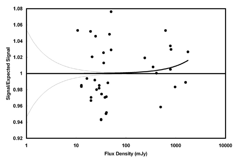
Figure B1: Normalized (to linear response) Signal vs. Flux Density at 24$\mu$m. Models for three different types of nonlinearity are compared with the data. The two light lines are nonlinearity due to residual positive or negative 50$\mu$Jy latent images. The heavy line is a linearity correction; the best fit suggests that the correction applied in the data pipeline may be slightly too large (but not at a significant level). However, there is no convincing argument for any significant nonlinearity over the range of the calibration measurements (10 - 50mJy).

Figure B1 shows the normalized ratio of 24$\mu$m to K flux density, vs. 24$\mu$m flux density. We exclude the two lowest measurements (of HD 172728). We also exclude the measurements of HD 47332 and HD 57336, the two highest measurements, because they may have faint excess emission. Since we have excluded the two highest and two lowest measurements, the bias on the results should be minimal.

We have considered three types of nonlinearity. The first is the typical gradual reduction of response in a simple integrating amplifier as the wells fill. The second is an over-correction for a nonlinearity of the first kind, so it just reverses the sign of the curve. The third is having a small latent image under the image of the star being measured. Since we have used custom flat fields to remove latents, the sign of the latent image could be either positive (adding to the star signal) or negative (subtracting from it). Examination of our data indicates that we can place an upper limit of about 50$\mu$Jy on any residual latent image.

As shown in Figure B1, the primary evidence for nonlinearity is a tendency for the bright stars to yield slightly larger signals than would be the case with a perfectly linear system. This offset is within the errors, but, if confirmed, it suggests that the correction for nonlinearity in large signals may be slightly too big (see Engelbracht et al. (2007) for further discussion). There is also evidence for a slight tendency to obtain larger net slopes with increasing integration time, an effect that would be consistent with the possible nonlinearity (Engelbracht et al. 2007). However, at the level of our measurements, 10 to 50mJy, these effects are negligible.

10 Appendix C. Measurements with Spitzer

This appendix discusses our measurement procedures for the Spitzer data. It also collects the samples of stars used for the various calculations in the paper, along with their key parameters.

10.1 Procedures at 8$\mu$m

One of us (J. Carpenter) re-reduced the measurements of our solar-type stars to put them on the identical basis as the calibration reductions of Reach et al. (2005). The 8$\mu$m solar analog calibration is based on the stars listed in Table C1. Fortunately, although some of the IRAC bands can have small offsets due to positioning of the measuring aperture, this effect is immeasurably small at 8$\mu$m (M. Silverstone, private communication), and we have ignored it. We thus only had to divide by the bandpass correction to convert to equivalent monochromatic flux density at 7.872$\mu$m. Since the SEDs of solar-type stars match very closely in this spectral region those of A stars, we applied the correction quoted by Reach et al. for an A1 star, 1.042.

10.2 Procedures at 24$\mu$m

To achieve the most accurate possible data reduction at 24$\mu$m, we have used a series of custom processing steps that have been developed by the MIPS team (discussed in more detail by Engelbracht et al. 2007). These steps are applied after standard pipeline processing. First, we remove the artifacts due to dust particles on the instrument pickoff mirror. Special flat fields are constructed from all of the photometric data to identify the effects of these particles. Second, we compensate for the latent images on the 24$\mu$m array as a result of exposure to bright sources. These dark latents appear as regions of reduced sensitivity centered on the array positions of bright sources in subsequent exposures. An image of the latents with all sources removed is produced by median combining the entire data set with appropriate bright source masks. The dark latents are removed from each individual frame by dividing the frames by the normalized dark latent image prior to mosaicking. Finally, mosaicked images are produced at the nominal pixel scale, 2.45”. This processing is described in more detail by Engelbracht et al. (2007).

We used simple aperture photometry on the 24$\mu$m images. The tabulated data assumed 1 DN/s = 1.05 mJy/square arcsec. The photometry was done within an aperture of radius 35”, and relative to sky measured in an annulus between radii of 40 and 50”. The aperture correction for this measurement approach was taken to be 1.084. We used the standard world coordinate system pointing information as a first guess for centering, with fine tuning with the IDL program ”mpfit2dpeak.pro” written by Craig Markwardt. Comparing photometry for separate measurements of the same star (typically also in different observation campaigns) indicates that the end-to-end scatter (including instrumental instability as well as photometry errors) is less than 0.5% rms (and not dependent on the brightness of the target for the range considered here – further discussion in Engelbracht et al. 2007). Achieving this level of repeatability requires not only the special post-pipeline processing, but also careful standardization of photometric procedures. Therefore, all the results reported in this paper used the identical photometric procedures applied by the same person (M. Blaylock). The results are listed in Tables C2 and C3; the maximum plausible errors in this band are no more than 1.5% rms.

Our procedures have been selected to be very conservative (e.g., large measurement aperture) and adapted to high repeatability. Other photometry approaches can be tested by using archival data for our program stars listed in Tables C2 and C3.

10.3 Color Combinations

Tables C1 - C3 list the 2MASS K_S value and a second K_S magnitude. $SuperK_{S}$ is a combination of the 2MASS J, H, and K_S measurements used to measure the scatter in K_S - [24] color among the stars. We used the standard colors for the spectral type of the star (Tokunaga 2000) to convert the J and H measurements to equivalent K_S ones. The typical distance to one of the A stars is about 100pc, so reddening may be significant. We estimated the reddening from the standard V-K color for the spectral type of the star (Tokunaga 2000) and the extinction curve of Rieke and Lebofsky (1985), and corrected all the J, H, and K measurements accordingly (the 24$\mu$m extinction is less than 1% even for the most obscured of the stars). The $SuperK_{S}$ magnitude is the weighted average of all three extinction- and color-corrected measurements. Because the colors of A stars are close to zero already, minor differences in photometric system have little influence on this conversion. The small offsets in the 2MASS J - K and H - K colors discussed in Appendix D have a negligible effect on our calculations here, because they are nearly equal and opposite in sign. The nominal errors in the resulting $SuperK_{S}$ magnitudes are 2% or less. Similar procedures were used to compute $SuperK_{S}$ for the solar-type stars in Tables C1 and C3, except that no extinction corrections were applied. Although some of the minor offsets in 2MASS have been mitigated by our using only Read 1 observations, there is little information over the full Read 1 dynamic range on how the photometry behaves at this level of accuracy. We therefore place an estimate of 3% on the net errors - half from the rms errors and half from possible systematic ones.

10.4 Procedure with IRS Data

To obtain a high signal-to-noise IRS spectrum of a solar-type star, we started with the spectra of the A stars HR 1014, 2194, 5467, and HD 163466 and of the solar-type stars HD 9826, 10800, 13974, 39091, 55575, 84737, 86728, 95128, 133002, 136064, 142373, 188376, 196378, 212330, and 217014 obtained from the Spitzer archive. After standard processing with the S13 IRS pipeline to the BCD level, nod pairs were subtracted to remove the background and the spectra were extracted with SPICE (Spitzer Science Center 2007). We then ratioed the spectra for similar stellar types in various combinations to determine the subset that were most closely similar. We also gave weight to evidence from the signal strength that the star was accurately centered in the spectrograph slit. As a result, we rejected HR 1014 from further processing because of a number of broad peaks and valleys in the ratio. We rejected the short module data for HD 9826, 95128, 188376 because of pronounced downward slopes with increasing wavelength in the ratios, and also HD 13974 and HD 196378 because the S module ratio is low relative to the L module data, suggesting a pointing issue with S. We rejected the L module data for HD 13974 and 188376 because of slopes and curves in the ratios, as well as for HD 9826, 95128, and HD 142373 because low values of the ratio relative to that for the S module suggest pointing issues. We averaged the accepted spectra (ten for each module) with equal weight, and then divided the solar-type average spectrum with the A-star one and multiplied the result by the A-star Kurucz model. The resulting spectrum had a discontinuity between the short and long IRS modules, which we removed by forcing the average value between 12 and 14$\mu$m to equal that between 15 and 17$\mu$m. We finally smoothed the result with a 7-pixel boxcar (giving a final spectral resolution of $\sim$ 10%).

11 Appendix D. JHK System

11.1 Vega and the Zero Point

Most near infrared photometric systems claim to be relative to a zero point defined by Vega, with this star or a model of it placed either at 0.02 (to coincide with the Johnson bright star measurements) or at zero. We have investigated how the peculiarities of this star have affected these definitions. This question is not easily answered because few of the sets of photometry since Johnson have actually measured Vega directly. We have therefore evaluated the quality of the Johnson photometry and then transformed it into the 2MASS system, finally using the transformation to compute the magnitude of Vega as it would have been measured by 2MASS.

Johnson et al. (1966) report 173 measurements of Vega within the overall set of photometry that constitutes their study of bright stars. We evaluated the quality of this photometry in two ways. First, we looked at the internal scatter for the individual measurements of Vega. We rejected the four highest and lowest measurements at both J and K (i.e., 4.6% of the measurements) and computed the straight average and standard deviation of the remaining 165 measurements. The results are J = 0.019 $\pm$ 0.004, K = 0.023 $\pm$ 0.004, and rms scatter of 0.048 and 0.050 in J and K respectively. With no outlier rejection the values for Vega are unaffected, but the errors increase to 0.005 and the rms scatter values to 0.061 and 0.065. However, we believe the values with the outlier rejection are the most representative.

We have tested this result in another way, by comparing stars measured in common by Johnson et al. (1966) and either Bouchet et al. (1991) or Kidger and Martín-Luis (2003). We first transformed the Johnson photometry into the other system (as described below). We excluded stars used by Johnson et al. (1966) as standards (stars such as Vega that were measured many times) in case their use in fitting for the photometric corrections would bias the comparison. There were 314 measurements suitable for the comparison with Bouchet et al. (1991), of which we rejected the seven high and seven low outliers (i.e., 4.5% of the measurements). The rms of the deviations was then 0.054 at J and 0.048 at K, that is, in excellent agreement with the internal scatter of the Johnson measurements of Vega. Similarly for the measurements of Kidger and Martín-Luis (2003), there were 135 suitable measurements. After transforming the Johnson photometry and rejecting the two high and two low outliers (3% of the measurements), the rms scatter is 0.048 at both J and K. We conclude that the Johnson et al. (1966) photometry is valid at the level of 1-$\sigma$ errors of 0.05 magnitudes for single measurements. Since most of the published bright star photometry is based on three or more measurements per star, this result is consistent with a typical overall accuracy of 3% or better.

The accuracy of the Johnson et al. (1966) photometry implies that Vega is tied into their overall photometric system to a 1-$\sigma$ error of less than 0.005 magnitudes. We will now determine transformations to put this measurement into the 2MASS Read 1 system. The simplest approach is to transfer directly. However, there are relatively few stars that were measured to high accuracy with the original Johnson photometer and that are faint enough not to saturate the 2MASS detector arrays. We have based the transformation on stars measured in Johnson et al. (1966, 1968) and in Lee (1968). The comparison is compromised by the decreased signal to noise of the stars and we have not attempted a color correction (although the data imply it would be small). We derive that Vega would have a 2MASS J magnitude of -0.042 and a K magnitude of -0.057. Given the issues with signal to noise, we prefer the average of these values, -0.050, as a best estimate of the near infrared Vega magnitude.

This result is limited by the poor overlap in the dynamic range of the two measurement sets; to overcome this problem, we have calculated the 2MASS Vega magnitudes by transforming the Johnson photometry to other systems that have a wider overlap with 2MASS. For the first case, we used bright standards in the CIT system defined by Elias et al. (1982). We find a transformation in good agreement with those derived previously by Elias et al. (1985) and Bessell and Brett (1988), although our procedure differed from theirs because we fitted the individual measurements of Johnson et al. (1966) not the final photometric results combining those measurements for each star. We use the transformation from the CIT to 2MASS systems available at the 2MASS web site to obtain 2MASS K_S magnitudes for Vega of -0.028, -0.023, and -0.032 using respectively our transformation and those of Besell & Brett (1988) and of Elias et al. (1985). Similarly, we obtain a 2MASS K_S magnitude of -0.033 if we make the transformation through the ESO system photometry of Bouchet et al. (1991) and a K_S magnitude of -0.045 if the transformation is made through the main body of photometry of Kidger & Martín-Luis (2003; their Table 2). There is a conflict in the latter case because Kidger & Martín-Luis (2003) also measured Vega directly, using a reduced system gain, and set it identically to zero magnitude at the near infrared bands (their Table 3). To check this result, we have computed the average K - L (rejecting one high and one low value) for the 19 late B stars and A stars using L from their Table 3 (in all cases measured with the reduced gain) and K from either Table 2 or 3. We obtain + 0.058 $\pm$ 0.016 where we would have expected zero. This result implies that the L magnitude of Vega if measured relative to the high-gain K photometry would be -0.058 $\pm$ 0.016, in agreement with the negative K magnitude derived from their Table 2. Although we have been unable to explain the discrepancy completely, the behavior of the other stars at L has led us to accept the value from the transformation of the data in Table 2. An additional comparison can be made from Koornneef (1983), who established a system based on the Johnson J and K photometry. From the 2MASS color transformations, the corresponding 2MASS K magnitude for Vega would be -0.023.

All of these estimates are consistent with assigning Vega the average K magnitude of -0.036 $\pm$ 0.006 in the 2MASS system. The quoted error is based on the scatter of the measurements; given the small number of them, an error of 0.010 is a more secure estimate.

11.2 2MASS Measurements

The 2MASS data provide a very homogeneous set of near infrared photometry over the entire sky, with accuracies well within the original specifications for the survey. Nonetheless, there are small offsets in those measurements that can be significant at the levels of accuracy desired for the calibration discussed in this paper. We discuss two such effects in this appendix.

11.2.1 Read1/Read 2 offset

There are offsets of the order of 2% between Read 1 and Read 2 measurements, in the range where they overlap. It is not clear how to derive a universal correction for this effect. Therefore, for the calibration we selected stars measured only in Read 1 mode.

11.2.2 Procedures for VJHK Calibration of A Stars

To define a zero point at V, J, H, and K, we built a sample of 57 A0V stars distributed over the entire sky, brighter than m_V = 7 mag., and with ”A” quality Read 1 2MASS measurements at all three near infrared colors. We took B and V magnitudes from the Hipparcos Main Catalog (Perryman et al. 1997). Stellar classifications were taken from SIMBAD. The infrared colors are not a strong function of the spectral type - from B8 to A2, J - K changes from -0.03 to +0.03 (Tokunaga 2000) - so type errors are not a major concern. However, reddening is. To eliminate reddened stars (and other sources of error), we excluded ones with B-V $>$ 0.05 and ones with $|$V - K_S$|$ $>$ 0.05. In addition, because the 2MASS quoted errors can be large in H band, we excluded three stars with H - K $>$ 0.07, which is 5% redder than the value averaged over the sample. For the final sample of 57 stars (see Table D1), the result was an average $<$V - K$>$ consistent with zero, $<$J - K$>$ = -0.022 $\pm$ 0.003, and $<$H - K$>$ = 0.019 $\pm$ 0.003. The average values are not affected by various assumptions we tried with regard to final sample selection. For example, if we keep all stars with $|$V - K$|$ $<$ 0.1, we get a slight positive residual in $<$V - K$>$, but values for $<$J - K$>$ and $<$H - K$>$ equal to the ones above within the errors.

An independent test was conducted with A0 dwarfs from the Michigan spectral atlas. There are a total of 6008 such stars with ”good” 2MASS measurements in all three bands. We discarded all of them with $|$V - K_S$|$ $>$ 0.05, leading to a sample of 510. Eleven of this sample were discarded as photometric outliers. Of the remaining stars, 220 have Read 1 photometry in all three bands, and the net J - K_S = -0.016 $\pm$ 0.018 for these stars. Similarly, we found a net H - K_S = +0.026 $\pm$ 0.022 based on 212 stars from the Michigan spectral atlas sample. The quoted errors are the population standard deviations. The nominal standard deviations of the means are only about 0.001, but there are suggestions of other low level trends in the data that would make such an accurate color difficult to obtain. We conclude that the net colors are in agreement with the ones derived from the smaller and more heterogeneous sample discussed above. The result for the stars measured in Read 2 mode are J - K_S = -0.005 $\pm$ 0.021 (population sigma, 150 stars) showing that the offset is a function of the 2MASS read mode. Therefore, corrections to remove these small effects will be relatively complex to apply. Cohen et al. (2003) have also identified offsets of similar size, but not with the same values as those we have determined. Their sample is predominantly K giants, and their Vega zero point model is redder than ours. If we compute the offsets only for the nine A stars in their sample and correct for the different colors for Vega, their results agree with ours to within 1.5 - 2% with errors of about 1.6%, i.e., within the errors.

These results could at least partially explain infrared color offsets such as those found by Casagrande et al. (2006; Figures 2,3, and 4). Future improvements in the comparisons with theoretical models will need to take account carefully of such small systematic effects in the photometry.

11.2.3 Procedures for Solar-Type Stars

In the V, J, H, and K bands, the colors of solar-type stars depart significantly from a Rayleigh-Jeans shape and we have to be careful in defining a sample of such stars. We determined average colors from the list of 36 solar-type stars in Table D2. The stellar parameters are from the Appalachian State Nstars web site (Gray 2007), with a few extras from Soubiran & Triaud (2004). A fit of temperature vs. spectral type from the full Nstars database shows that the average G2V star is assigned a temperature of 5720K. The solar temperature of 5778K is within the scatter, but either the sun is relatively hot for its spectral class, or there is a systematic offset between its temperature and those assigned through the stellar models to other stars.

We used the Hipparcos photometry at V to eliminate stars from the sample with V - K_S colors differing by more than 0.1 magnitudes from expectations for their spectral types. These stars are systematically much closer than the A stars discussed above, so the color deviations are less likely to arise from reddening. In support of this conclusion, there are nearly as many blue as red deviations. We attribute the discordant values to errors in the spectral types.

Each V - K_S was corrected to the equivalent value for 5778K according to a relationship fitting the temperature of the star and the standard V - K colors from Tokunaga (2000). This relationship was set to zero at 5778K, so it acts only to take out the variations with temperature but not to cause an overall shift in color. We ignored reddening because the maximum distance of the sample members, 40pc, puts them within the Local Bubble of very low density interstellar medium (e.g., Knude & Hog 1998 and references therein).

Although we prefer to use the Hipparcos V magnitudes because they are homogeneous over the entire sky, to do so we need to allow for possible systematic offsets relative to Johnson V. These effects should be small for A stars because of their nearly zero colors. To evaluate them for solar-type stars, we used the sample of 102 stars listed in the Nstars database as being of G-type and for which there was high quality V photometry, to find a net offset of $<$V_Hipp - V_Johnson$>$ = -0.007 $\pm$ 0.002. We corrected the measured V - K_S color accordingly. We also found two stars in our solar-type sample, HD 139777 and HD 218739, with large offsets between the Nstars tabulated groundbased magnitudes and those from Hipparcos (0.07 - 0.08 mag.). Multiple groundbased measurements plus the V - K color showed that the groundbased results were correct, and we substituted them. Otherwise, the standard deviation in the difference of Hipparcos and groundbased V magnitude derived from uvby was only 1.6%, confirming the high quality of the Hipparcos data (and of the groundbased uvby data also).

12 Appendix E. Calculation of Effective, Nominal, and Isophotal Wavelengths

Given R($\lambda$) as the relative response function of the photometric band, the equivalent band width is

$$BW=\frac{{1}}{{R_{max}}}\int{R\left({\lambda}\right)\;d\lambda}$$ (1)

where R_max is the maximum value of R($\lambda$) (often R($\lambda$) is normalized to 1). The average flux in the band is

$$\left\langle{F_{\lambda}}\right\rangle=\frac{{\int{\lambda\;F_{\lambda}\left({\lambda}\right)\;R\left({\lambda}\right)\;d\lambda}}}{{\int{\lambda\;R\left({\lambda}\right)\;d\lambda}}}\;,$$ (2)

or equivalently is the total flux passed by the band divided by the band width.

To idealize measurements made through a given photometric band to a monochromatic equivalent flux, we need to assign a specific wavelength to the measurement. The mean, or effective, wavelength is defined by the following equation:

$$\lambda_{0}=\frac{{\int{\lambda}\,R\left(\lambda\right)\;d\lambda}}{{\int R\left({\lambda}\right)\;d\lambda}}.$$ (3)

Examples are given in Table 6. The zero point (ZP) is conventionally defined as the flux density of ”Vega” at $\lambda_{0}$, but the stellar absorption features pose complications. The ZPs in Table 6 are determined by interpolating over the absorptions in the stellar spectrum and then averaging $\lambda^{4}F_{\lambda}$ over a 1% bandpass. Any measurement expressed in terms of the mean wavelength of the photometric band needs to be accompanied by a color correction term that converts the apparent flux density to the value at $\lambda_{0}$ for the specific source spectral energy distribution that reproduces the observed signal strength (e.g., Low & Rieke 1974). The color correction is normalized to the result for a source with F_λ($\lambda$) = constant across the band. The absorption features in stellar spectra can make computation of a precise color correction problematical, but alternatively one can be based on a blackbody spectrum. We have taken this approach for the illustrative values in Table 6. They are given in the sense that a flat spectrum that gives the same signal as a blackbody of the specified temperature will be brighter at the mean wavelength by the tabulated factor. It is convenient in many cases to set the color correction to zero for hot stars, which can be accomplished by an offset in the set of color terms with an appropriate counter-adjustment in the nominal zero point flux density (e.g., Low and Rieke 1974; MIPS Handbook).

Another way to circumvent the effects of stellar absorptions is to use the ”average zero point”, $\left\langle{F_{\lambda}}\right\rangle$, where the flux density is that of ”Vega”. Where the stellar spectrum is smooth and follows a Planck curve closely, the average flux in the band is reproduced reasonably well by the stellar flux density at the mean wavelength times the color correction. Where the stellar spectrum deviates from Planckian behavior (e.g., in the H band due to the many members of the Brackett series), there may be significant deviations from this relation. In general cases, the use of a fiducial wavelength and zero point imposes limits in the achievable accuracy; it may be required to carry out the relevant integrals of the relative response function convolved with the object spectra.

Under many conditions, the value of the required color correction can be minimized by modifying the wavelength associated with the band to the ”nominal wavelength” (Reach et al. 2005), defined as

$$\lambda_{0}^{\prime}=\frac{{\int{\lambda^{2}\;R\left({\lambda}\right)\;d\lambda}}}{{\int{\lambda\;R\left({\lambda}\right)\;d\lambda}}}\,.$$ (4)

Table 6 includes the ZP flux densities appropriate to this definition. Color corrections under this definition are relative to those for a source with F_λ($\lambda$) $\propto\lambda$. Otherwise, the procedures and pitfalls are similar to those for the mean wavelength.

The definitions in equations (3) and (4) have the advantages that they are simple in concept and that the wavelength associated with a band is independent of the source properties. Yet another definition is the isophotal wavelength, defined by

$$F_{\lambda}\left({\lambda_{iso}}\right)=\left\langle{F_{\lambda}.}\right\rangle$$ (5)

This approach has the advantage of subsuming the correction terms into the wavelength specification, providing a more streamlined description of a measurement. However, it is potentially confusing to have different wavelengths associated with measurements of different sources in the identical photometric band, and relating measurements to the identical wavelength requires introduction of color corrections similar to those needed with the definitions in equations (3) and (4) (Tokunaga & Vacca 2005).

The issue of stellar features is complex in the use of $\lambda_{iso}$, where the basic definitions can be misleading (e.g., F_λ($\lambda$_iso) may depend on the resolution used to measure the spectrum of the source). To avoid this difficulty, one must use a continuum model of the stellar spectrum or interpolate over its spectral features. Golay (1974) suggests avoiding these difficulties by replacing the stellar spectrum with a suitable Planck function. Instead, for the 2MASS bands we have interpolated over any lines close to the fiducial wavelength (a procedure similar to that used by Cohen et al. 1992, 2003). We find that reliable interpolations can be based on $\lambda$⁴ F_λ. Since the infrared is close to the Rayleigh-Jeans realm for Vega, the resulting function varies slowly and smoothly with wavelength, making it appropriate to use linear interpolations across line-contaminated regions. The interpolated values were converted to flux by dividing by $\lambda$⁴. Figures E1 - E3 show our interpolations on the model spectrum of ”Vega”. Table E1 lists the beginning and end wavelengths for the interpolations. Our calculated values of $\lambda$_iso in Table 6 agree closely with those of Cohen et al. (2003). Therefore, many aspects of their analysis, such as the water vapor dependence of the nominal bands and fiducial wavelengths, can be applied to our proposed calibration without change.

For the mid-infrared space missions, color corrections as a function of source spectral characteristics can be found in the appropriate user handbooks. The MIPS calibration is to a mean wavelength, while the IRAC and IRAS ones are to a nominal wavelength. Because these corrections are tracked as official project values, we quote our results in a form that assumes they will be used as tabulated.

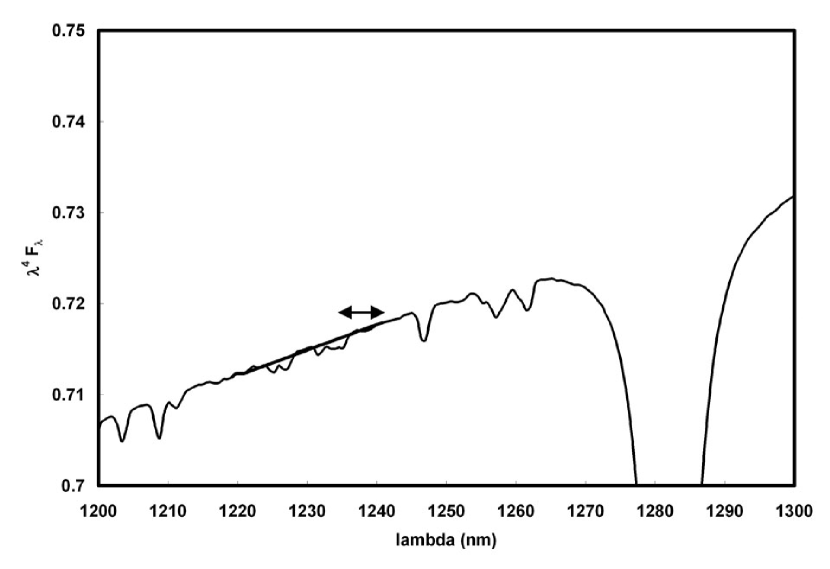
Figure E1: Interpolation over spectral absorptions in the J band. The horizontal arrow shows the approximate range of the various band-defining wavelengths.

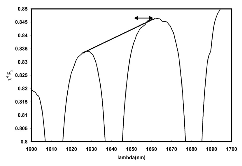
Figure E2: Interpolation over spectral absorptions in the H band. The horizontal arrow shows the approximate range of the various band-defining wavelengths.

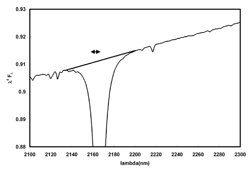
Figure E3: Interpolation over spectral absorptions in the K_S band. The horizontal arrow shows the approximate range of the various band-defining wavelengths.

Table 1: Absolute Flux Density from ”Vega” at 10.6 and 24$\mu$m

Approach	Flux Density	Error
	@ 10.6$\mu$m (Jy)	(Jy)
Rieke et al. (1985)	35.3	1.1
MSX weighted average	35.04	0.24
Weighted average of Rieke, MSX	35.05	0.23
Solar analog (this work)	34.53	1.1
All measurements weighted average	35.03	0.23
Average Rieke et al., solar analog	34.92	0.8
Adopted	35.03	0.3
Adopted, Fλ	9.35X10-17 W cm-2 $\mu$m-1
Hammersley et al. 1998	35.2	–
Flux Density at 23.675$\mu$m	7.17	0.11

Table 2: Measurements of the Absolute Flux of ”Vega” at 2.22$\mu$m

Reference	Equivalent 2.22$\mu$m	Error
	Flux Density (Jy)	(Jy)
Walker (1969)	638	64
Blackwell et al. (1983)	666	20
Selby et al. (1983)	623	25
Booth et al. (1989)	667	27
Weighted average	653	13
Corrected for disk	645	15
Extrapolated from 10.6$\mu$m	649	10
”best” calibration	647	8

Table 3: Comparison of Solar and Stellar Colors

Band	Synthetic Solar	Observed,	HM74	Fontenla et al.
	Color (mag)	Solar-Type Stars	Model	2006 Model
VJ	0.00	0.00		0.00
V-J	1.158 $\pm$ 0.02	1.158 $\pm$ 0.015		1.20
V-H	1.513 $\pm$ 0.02	1.484 $\pm$ 0.020		1.55
V-KS	1.568 $\pm$ 0.02	1.545 $\pm$ 0.015	1.550	1.57
V-$\rm{[8]}$	1.596 $\pm$ 0.02	1.591 $\pm$ 0.015	1.596*	1.615
V-$\rm{[24]}$	1.54 $\pm$ 0.05	1.590 $\pm$ 0.020	1.577	1.564

Note. — *Adopted value, since model does not extend below 2$\mu$m; the Thuillier et al. SED was used to fill in the 1.927 - 2.00$\mu$m range not included in the model.

Table 4: Solar analog colors corrected to our system from Bessell et al. (1998)

	$V-K_{S}$	Reference
Sun-ref	1.574	Colina et al. 1996
Analog	1.563	Cayrel de Strobel 1996, Table 6
Model	1.587	SUN-OVER*
Model	1.587	SUN-NOVER*
	from Table 3
Solar Spectrum	1.568$\pm$ 0.02	V, KS from Thuillier et al. 2003
Model	1.57	Fontenla et al. 2006
ATLAS9 Model	1.556	Casagrande et al. 2006
Kurucz 2004	1.555	Casagrande et al. 2006
MARCS Model	1.547	Casagrande et al. 2006
Solar-Type Stars	1.545$\pm$0.02	This work
	NICMOS prime calibrator
P330E	1.577	Bohlin et al. 2001

Note. — *Terminology from Bessel et al. (1998); SUN-OVER refers to ATLAS9 models with overshooting turned on, while SUN-NOVER has it turned off.

Table 5: Multiplicative Factors to Reconcile Mid-IR Calibrations to Proposed One

2MASS KS	IRAC 7.872$\mu$m	IRAS 12$\mu$m	IRAS 25$\mu$m
1.02*	1.015**	0.992	0.980

Note. — *Relative to calibration of Cohen et al. (2003). **Relative to calibration of Reach et al. (2005)

Table 6: Suggested calibration of 2MASS photometry

Band	J
Band Width	0.1625$\mu$m
Average Zero Point (ZP) (W cm-2 $\mu$m-1)	3.21 X 10-13
Wavelength Type	$\lambda_{0}$ ($\mu$m)	$\lambda_{0}$’ ($\mu$m)	$\lambda_{iso}$ ($\mu$m)
Wavelength	1.2410	1.2444	1.2356
ZP Fλ at $\lambda_{0}$ (W cm-2 $\mu$m-1)	3.16X10-13	3.13X10-13	3.21X10-13
ZP Fν at fiducial $\lambda$ (Jy)	1623	1617	1635
Color Correction/9550K Black Body	1.017	1.028
Band	H
Band Width	0.2508$\mu$m
Average ZP (W cm-2 $\mu$m-1)	1.164 X 10-13
Wavelength Type	$\lambda_{0}$ ($\mu$m)	$\lambda_{0}$’ ($\mu$m)	$\lambda_{iso}$ ($\mu$m)
Wavelength	1.6513	1.6551	1.6597
ZP Fλ at fiducial $\lambda$ (W cm-2 $\mu$m-1)	1.182X10-13	1.174X10-13	1.163X10-13
ZP Fν at fiducial $\lambda$ (Jy)	1075	1073	1068
Color Correction/9550K Black Body	1.014	1.023
Band	KS
Band Width	0.2620$\mu$m
Average ZP (W cm-2 $\mu$m-1)	4.37X10-14
Wavelength Type	$\lambda_{0}$ ($\mu$m)	$\lambda_{0}$’ ($\mu$m)	$\lambda_{iso}$ ($\mu$m)
Wavelength	2.1657	2.1692	2.1598
ZP Fλ at fiducial $\lambda$ (W cm-2 $\mu$m-1)	4.32X10-14	4.30X10-14	4.36X10-14
ZP Fν at fiducial $\lambda$ (Jy)	676	675	678
Color Correction/9550K Black Body	1.018	1.030

Table A1: Reference Spectral Energy Distributions of the Sun and Vega

Wavelength	Sun	Vega
$\mu$m	W m-2 nm-1	W m-2 nm-1
0.1998	$7.520\times 10^{-3}$	$5.581\times 10^{-11}$
0.2017	$8.160\times 10^{-3}$	$5.312\times 10^{-11}$
0.2035	$9.120\times 10^{-3}$	$5.165\times 10^{-11}$
0.2052	$1.077\times 10^{-2}$	$5.752\times 10^{-11}$

Table C1: Solar Type 8$\mu$m Calibration Sample.

Name	Type	$SuperK_{S}$	KS	f(8$\mu$m)	flux ratio*
		(mag)	(mag)	(mJy)
HD 00643	G2/G3V	6.204	6.187	215.1	0.99
HD 00894	F8IV-V	5.353	5.378	448.8	0.98
HD 01901	F8	5.563	5.57	371.6	0.97
HD 02746	G5	6.262	6.282	198.5	1.00
HD 03796	G4V	6.279	6.268	198.2	0.98
HD 03894	G1V	6.419	6.442	172.3	1.00
HD 06073	G0	6.246	6.253	202.1	0.99
HD 08820	G0IV-V	6.114	6.118	229.9	0.99
HD 08874	G1V	4.967	4.955	663.2	0.98
HD 09071	G2/G3V	6.054	6.042	235.4	0.95
HD 09278	G5	5.724	5.721	322.7	0.96
HD 09855	G2/G3V	6.072	6.078	238.8	0.99
HD 10195	G0V	5.611	5.609	361.3	0.97
HD 10625	G0V	5.940	5.929	270.9	0.98
HD 10879	G1/G2V	4.857	4.832	767.1	1.01
HD 10894	F8	6.009	6.025	256.9	1.02
HD 11219	F8V	5.556	5.553	395.6	1.01
HD 11504	G1Va	5.331	5.334	476.0	1.00
HD 12150	G2V	6.135	6.124	225.3	0.98
HD 12265	F8	5.863	5.879	283.1	0.98
HD 14193	G2/G3V	5.771	5.764	310.8	0.97
HD 15070	G0	5.572	5.565	388.1	1.01
HD 15922	G5V	4.981	4.998	613.3	0.94
HD 17994	F8V	4.952	4.936	658.4	0.96
HD 18321	G2V	5.754	5.766	320.8	1.00
HD 19301	F8	5.945	5.966	264.7	0.99
HD 19503	G5	5.561	5.579	379.4	1.00
HD 19959	G0V	5.462	5.461	412.2	0.97
HD 20427	F8V	5.412	5.449	415.8	0.97
HD 20590	G4IV-V	5.314	5.321	491.1	1.02
HD 21229	G5	6.265	6.269	206.0	1.02
HD 21627	G0	5.782	5.794	309.5	0.99

Note. — *Ratio of observed flux density to expected flux density from the photosphere. See Rieke et al. (2005) and Su et al. (2006) for further details.

Table C2: A-Type Stars Used to Determine the K_S - [24] Zero Point.

Name	Age	V	$SuperK_{S}$	KS	f(24$\mu$m)	flux ratio*
	(Myr)	(mag)	(mag)	(mag)	(mJy)
HD 319	600	A1V	5.467	5.479	45.89	0.99
HD 02811	750	A3V	7.067	7.057	10.94	1.01
HD 11413	600	A1V	5.396	5.422	53.13	1.08**
HD 14943	850	A5V	5.469	5.439	48.92	1.01
HD 15646	260	A0V	6.398	6.411	20.15	1.02
HD 17254	650	A2V	5.907	5.877	31.12	0.97
HD 17254	650	A2V	5.907	5.877	30.47	0.94
HD 20888	300	A3V	5.723	5.691	37.02	0.97
HD 20888	300	A3V	5.744	5.691	38.28	1.00
HD 21981	265	A1V	5.513	5.526	41.35	0.93
HD 34868	300	A0V	6.018	6.024	26.3	0.93
HD 42525	300	A0V	5.763	5.751	34.76	0.96
HD 57336	400	A0IV	7.188	7.114	9.544	0.92
HD 73210	729	A5V	6.170	6.165	24.96	1.01
HD 73666	729	A1V	6.524	6.532	18.11	1.03
HD 73819	729	A6Vn	6.322	6.28	21.42	0.96
HD 92845	300	A0V	5.519	5.513	47.71	1.06**
HD 101452	250	A2	6.799	6.819	13.01	0.96
HD 105805	500	A4Vn	5.626	5.6	38.96	0.94
HD 116706	500	A3IV	5.507	5.502	42.03	0.92
HD 128998	250	A1V	5.758	5.756	32.73	0.91
HD 158485	420	A4V	6.153	6.145	24.30	0.96
HD 163466	310	A2	6.300	6.339	19.48	0.92
HD 163466	310	A2	6.300	6.339	20.03	0.95
HD 172728	210	A0V	5.746	5.753	32.33	0.89***
HD 172728	210	A0V	5.746	5.753	32.3	0.89***

Note. — *Ratio of observed flux density to expected flux density from the photosphere. See Rieke et al. (2005) and Su et al. (2006) for further details. **Possible weak 24$\mu$m excess. ***Low value probably reflects a measurement error, possibly in the 2MASS K_S magnitude.

Table C3: Solar Type 24$\mu$m Calibration Sample.

Name	age	Type	$SuperK_{S}$	KS	f(24$\mu$m)	flux ratio*
	(Myr)		(mag)	(mag)	(mJy)
HD 008941	2200	F8IV-V	5.353	5.378	49.2	0.96
HD 019019	1700	F8	5.563	5.57	42.4	0.99
HD 027466	1500	G5	6.262	6.282	21.5	0.97
HD 037962	2400	G4V	6.279	6.268	22.4	1.00
HD 038949	1000	G1V	6.419	6.442	19.6	1.02
HD 064324	1700	G0	6.234	6.235	25.1	1.08
HD 066751	4200	F8	5.061	5.066	66.1	0.97
HD 092788	6800	G5	5.724	5.721	36.2	0.97
HD 098553	5800	G2/G3V	6.072	6.078	26.4	0.98
HD 100167	2300	F8	5.826	5.806	34.4	1.00
HD 101472	1100	G0	6.125	6.139	26.2	1.03
HD 101959	4700	G0V	5.611	5.609	39.8	0.96
HD 106252	5000	G0V	5.940	5.929	32.4	1.06
HD 108799	9300	G1/G2V	4.857	4.832	84.9	1.01
HD 108944	4500	F8	6.009	6.025	30.3	1.08
HD 112196	7300	F8V	5.556	5.553	43.4	1.00
HD 115043	11500	G1Va	5.331	5.334	53.7	1.01
HD 121504	7100	G2V	6.135	6.124	27.4	1.07
HD 122652	2500	F8	5.863	5.879	34.8	1.08
HD 141937	4500	G2/G3V	5.771	5.764	35.0	0.98
HD 150706	1400	G0	5.572	5.565	45.5	1.06
HD 153458	1400	G0	6.449	6.447	19.1	1.00
HD 159222	3800	G5V	4.981	4.998	68.3	0.94
HD 167389	2200	F8	5.910	5.918	30.4	0.98
HD 193017	1900	F8	5.945	5.966	28.4	0.95
HD 195034	4800	G5	5.561	5.579	41.9	0.99
HD 199598	2100	G0V	5.462	5.461	48.0	1.01
HD 204277	1100	F8V	5.412	5.449	49.9	1.04
HD 205905	1500	G4IV-V	5.314	5.321	53.8	1.00
HD 212291	2900	G5	6.265	6.269	22.7	1.01
HD 216275	4400	G0	5.782	5.794	34.6	0.99

Note. — *Ratio of observed flux density to expected flux density from the photosphere. See Rieke et al. (2005) and Su et al. (2006) for further details.

Table D1: Near Infrared Colors of A Stars in 2MASS Read 1 Mode.

Name	V	B - V	V - K	J - K	H - K
HD 012468	6.52	0.003	-0.037	-0.05	0.016
HD 021379	6.29	-0.025	-0.021	-0.029	0.01
HD 022789	6.01	-0.027	0.002	0	0.057
HD 029526	5.66	0.002	0.011	0.014	0.019
HD 031069	6.06	-0.032	-0.047	-0.059	-0.004
HD 035505	5.64	-0.001	-0.009	-0.002	0.029
HD 035656	6.41	-0.023	-0.028	-0.044	-0.02
HD 036473	5.53	0.012	0.016	0.032	0.006
HD 041076	6.09	-0.035	0.002	0.004	0.035
HD 042301	5.49	-0.01	0.037	0.008	0.034
HD 042729	6.08	-0.021	0.051	0.004	0.05
HD 043583	6.59	-0.036	-0.031	-0.057	-0.009
HD 045137	6.51	-0.027	0	-0.011	-0.005
HD 045557	5.78	-0.001	0.026	0.001	0.049
HD 056386	6.19	-0.024	0.018	-0.042	0.016
HD 060629	6.64	-0.007	-0.015	-0.03	0.027
HD 070175	7	-0.01	-0.009	-0.001	0.035
HD 071043	5.89	0.018	0.017	-0.011	-0.002
HD 072337	5.51	-0.024	-0.04	-0.008	0.028
HD 076346	6.02	-0.023	-0.024	-0.004	0.003
HD 078955	6.53	0.001	0.041	0.018	0.062
HD 079108	6.14	-0.01	0.021	0.023	0.044
HD 080950	5.86	-0.024	-0.005	0.035	0.055
HD 086087	5.71	0.006	-0.027	-0.035	0.028
HD 096338	6.82	0.043	0.051	0.009	-0.007
HD 102981	6.62	-0.027	-0.021	-0.026	0.03
HD 104430	6.16	-0.004	-0.034	-0.01	-0.015
HD 107655	6.21	-0.012	0.043	-0.049	-0.029
HD 107947	6.61	-0.001	-0.008	-0.037	0.032
HD 113457	6.64	0.006	0	-0.032	0.007
HD 115527	6.87	-0.006	-0.007	-0.032	0.011
HD 117651	6.36	-0.014	-0.006	-0.044	0.03
HD 118214	5.6	-0.014	-0.035	-0.035	0.018
HD 121409	5.7	-0.032	0.022	-0.03	0.03
HD 124683	5.53	0.001	-0.022	-0.009	-0.004
HD 131951	5.9	-0.031	0.001	-0.048	0.02
HD 136831	6.29	-0.008	0.042	-0.031	0.008
HD 140729	6.15	0.002	0.019	-0.054	-0.016
HD 143488	6.99	0.006	0.023	-0.022	0.042
HD 145122	6.13	-0.003	0.046	-0.032	0.005
HD 145454	5.44	-0.019	0.009	-0.058	-0.003
HD 154972	6.24	-0.004	0.02	-0.011	0.014
HD 155379	6.52	-0.037	0	-0.007	-0.029
HD 172728	5.74	-0.045	-0.013	-0.028	0.02
HD 176425	6.21	0.001	-0.018	-0.024	0.064
HD 177406	5.95	-0.017	-0.014	-0.006	0.031
HD 178207	5.4	-0.014	-0.014	-0.046	0.032
HD 179933	6.26	0.008	0.001	-0.048	0.003
HD 182761	6.31	-0.014	0.023	-0.045	0.031
HD 182919	5.6	-0.006	-0.013	-0.038	0.014
HD 195549	6.35	0.001	0.007	-0.007	0.017
HD 205314	5.77	-0.042	-0.018	-0.055	0.025
HD 207636	6.45	-0.007	0.033	-0.015	0.026
HD 212643	6.29	-0.021	0.005	-0.028	-0.006
HD 219290	6.32	-0.005	-0.001	-0.024	-0.006
HD 219485	5.89	-0.01	0.018	-0.035	0.026
HD 223386	6.33	-0.007	-0.001	-0.03	-0.005

Table D2: Properties of Solar Analog Stars.

Name	Teff	log(g)	M/H	V - KS
Sun	5778	4.44	0	1.57
HD 001562	5756	4.43	-0.22	1.54
HD 003821	5785	4.40	-0.07	1.50
HD 008262	5861	4.34	-0.13	1.57
HD 009986	5749	4.39	-0.03	1.55
HD 010086	5659	4.61	-0.02	1.62
HD 010145	5673	4.40	-0.01	1.64
HD 011131	5819	4.53	-0.02	1.57
HD 012846	5667	4.38	-0.25	1.60
HD 020619	5666	4.50	-0.25	1.58
HD 041330	5858	4.25	-0.20	1.52
HD 042618	5714	4.58	-0.16	1.55
HD 063433	5691	4.60	-0.03	1.64
HD 071148	5756	4.35	-0.02	1.49
HD 073350	5754	4.37	0.04	1.52
HD 075767	5741	4.42	-0.08	1.57
HD 088072	5746	4.31	0.01	1.55
HD 089269	5674	4.40	-0.23	1.65
HD 090508	5779	4.24	-0.23	1.55
HD 114174	5750	4.34	0.07	1.58
HD 139777	5703	4.55	-0.05	1.50
HD 142093	5859	4.55	-0.15	1.49
HD 146946	5854	4.21	-0.21	1.62
HD 147044	5849	4.29	-0.03	1.45
HD 159222	5788	4.25	0.12	1.52
HD 165401	5798	4.27	-0.29	1.55
HD 166435	5741	4.41	-0.07	1.52
HD 168009	5801	4.09	-0.04	1.54
HD 177082	5733	4.25	-0.11	1.60
HD 186427	5753	4.25	0.06	1.60
HD 187237	5788	4.61	0.06	1.53
HD 196850	5792	4.30	-0.12	1.53
HD 197076	5842	4.34	-0.02	1.51
HD 202108	5665	4.38	-0.30	1.57
HD 217813	5861	4.41	-0.03	1.50
HD 218739	5788	4.41	0.06	1.44
HD 224465	5664	4.22	-0.12	1.58

Table E1: Beginning and end wavelengths for isophotal interpolations

	Beginning	End
J	1.221$\mu$m	1.240$\mu$m
H	1.6255$\mu$m	1.660$\mu$m
KS	2.134$\mu$m	2.200$\mu$m

References

- (1) 2MASS Web site: http://www.ipac.caltech.edu/2mass/
- (2) Absil, O., et al. 2006, A&A, 452, 237
- (3) Anders, E., Grevesse, N., 1989, Geochimica et Cosmochimica Acta 53, 197
- (4) Aufdenberg, J. P., et al. 2006, ApJ, 645, 664
- (5) Aumann, H. H., et al. 1984, ApJL, 278, 23
- (6) Ayres, T. R., Plymate, C., & Keller, C. U. 2006, ApJS, 165, 618
- (7) Becklin, E. E., Hansen, O., Kieffer, H., and Neugebauer, G. 1973, AJ, 78, 1063
- (8) Beichman, C. A., Neugebauer, G., Habing, H. J., Clegg, P. E., and Chester, T. J. 1988, IRAS Explanatory Supplement, NASA: Washington, D. C. Section VI. C.2.a
- (9) Bell, K.L., & Berrington, K.A., 1987, J. Phys. B20, 801
- (10) Bessell, M. S., & Brett, J. M. 1988, PASP, 100, 1134
- (11) Bessell, M. S., Castelli, F., and Plez, B. 1998, A&A, 333, 231
- (12) Bessell, M. S. 2005, ARAA, 43, 293
- (13) Blackwell, D. E., Leggett, S. K., Petford, A. D., Mountain, C. M., & Selby, M. J. 1983, MNRAS, 205, 897
- (14) Bohlin, R. C. 2007, in The Future of Photometric Systems,” PASP, 364, 315
- (15) Bohlin, R. C., Dickinson, M. E., and Calzetti, D. 2001, AJ, 122, 2118
- (16) Bohlin, R. C., and Gilliland, R. L. 2004, AJ, 127, 3508
- (17) Booth, A. J., Selby, M. J., Blackwell, D. E., Petford, A. D., & Arribas, S. 1989, A&A, 218, 167
- (18) Bouchet, P., Schmider, F. X., and Manfroid, J. 1991, A&AS, 91, 409
- (19) Campins, H., Rieke, G. H., & Lebofsky, M. J. 1985, AJ, 90. 896
- (20) Carpenter, J. M. 2001, AJ, 121, 2851
- (21) Casagrande, L., Portinari, L., & Flynn, C. 2006, MNRAS, 373, 13
- (22) Carter, B. S. 1990, MNRAS, 242, 1
- (23) Cayrel de Strobel, G., 1996, A&A Rev. 7, 243
- (24) Ciardi, D. R., van Belle, G. T., Akeson, R. L., Thompson, R. R., Lada, E. A., and Howell, S. B. 2001, ApJ, 559, 1147
- (25) Cohen, M., Walker, R. G., Barlow, M. J., and Deacon, J. R. 1992, AJ, 104, 1650
- (26) Cohen, M., Wheaton, W. A., & Megeath, S. T. 2003, AJ, 126, 1090
- (27) Colina, L., Bohlin, R. C., and Castelli, F. 1996, AJ 112, 307
- (28) Cutri, R. M. et al. 2003, The IRSA 2MASS All-Sky Point Source Catalog
- (29) Decin, L., 2000, PhD Thesis, University of Leuven (Belgium)
- (30) Decin, L., Vandenbussche, B., Waelkens, C., Eriksson, K., Gustafsson, B., Plez, B., Sauval, A.J., and Hinkle, K., 2003, A&A 400, 679
- (31) Elias, J. H., Frogel, J. A., & Humphreys, R. M. 1985, ApJS, 57, 91
- (32) Elias, J. H., Frogel, J. A., Matthews. K., and Neugebauer, G. 1982, AJ, 87, 1092
- (33) Engelke, C. W. 1992, AJ, 104, 1248
- (34) Engelbracht, C., et al. 2007, PASP, 119, 994
- (35) Fazio, G. G., et al. 2004, ApJS, 154, 39
- (36) Fontenla, J. M., Avrett, E., Thuillier, G., and Harder, J. 2006, ApJ, 639, 441
- (37) Golay, M. 1974, Introduction to Stellar Photometry, (D. Reidel: Dordrecht), p. 40
- (38) Gray, R. O. 1998, PASP, 116, 482
- (39) Gray, R. O. 2007, http://stellar.phys.appstate.edu/
- (40) Gulliver, A. F., Hill, G., & Adelman, S. J. 1994, ApJL, 429, L81
- (41) Hammersley, P. L., Jourdain de Muizon, M., Kessler,M. F., Bouchet, P., Joseph, R. D., Habing, H. J., Salama, A., & Metcalfe, L. 1998, A&AS, 128, 307
- (42) Harris, M.J., Lambert, D.L., & Goldman, A., 1987, MNRAS224, 237
- (43) Holmberg, J., Flynn, C., and Portinari, L. 2006, MNRAS, 367, 449
- (44) Holweger, H. and Müller E.A., 1974, Solar Physics 39, 19
- (45) Johnson, H. L. 1965a, Comm. Lunar Plan. Lab., 3, 73
- (46) Johnson, H. L. 1965b, ApJ, 141, 923
- (47) Johnson, H. L., and Morgan, W. W. 1953, ApJ, 117, 313
- (48) Johnson, H. L., Iriarte, B., Mitchell, R. I., and Wisniewski, W. Z. 1966, Comm. Lunar Plan. Lab., 4, 99
- (49) Johnson, H. L., MacArthur, J. W., & Mitchell, R. I. 1968, ApJ, 152, 465
- (50) Kidger, M. R., & Martín-Luis, F. 2003, AJ, 125, 3311
- (51) Knude, J., & Hog, E. 1998, A&A, 338, 897
- (52) Koornneef, J. 1983, A&AS, 51, 489
- (53) Kurucz, R. L. 2005, http://kurucz.harvard.edu
- (54) Labs, D. & Neckel, H. 1968, Zeitschrift fúr Astrophysik, 69, 1
- (55) Labs, D. & Neckel, H. 1970, Solar Physics, 15, 79
- (56) Lee, T. A. 1968, ApJ, 152, 913
- (57) Low, F. J., and Rieke, G. H. 1974, in Methods of Experimental Physics, Vol. 12, Part A, edited by N. Carleton (Academic: New York) p. 456
- (58) Maltby, P., Avrett, E. H., Carlsson, M., Kjeldseth-Moe, O., Kurucz, R. L., & Loesser, R. 1986, ApJ, 306, 284
- (59) Mégessier, C. 1995, A&A, 296, 771
- (60) MIPS Data Handbook: http://ssc.spitzer.caltech.edu/mips/dh
- (61) Mountain, C. M., Selby, M. J., Leggett, S. K., Blackwell, D. E., & Petford, A. D. 1985, A&A, 151, 399
- (62) NASA/IPAC Infrared Science Archive 2007, http://irsa.ipac.caltech.edu/data/SPITZER/FEPS/
- (63) Perryman, M. A. C. et al. 1997, A&A, 323, L49
- (64) Plez, B., Smith, V.V., Lambert, D.L., 1993, ApJ 418, 812
- (65) Price, S. D., Paxson, C., Engelke, C., & Murdock, T. L. 2004, AJ, 128, 889
- (66) Price, S. D. 2004, Space Science Reviews, 113, 409
- (67) Reach, W. T. et al. 2005, PASP, 117, 978
- (68) Rieke, G. H., Lebofsky, M. J., & Low, F. J. 1985, AJ, 90, 900
- (69) Rieke, G. H., & Lebofsky, M. J. 1985, ApJ, 288, 618
- (70) Rieke, G. H. et al. 2004, ApJS, 154, 25
- (71) Rieke, G. H. et al. 2005, ApJ, 620, 1010
- (72) Saiedy, F. 1960, MNRAS, 121, 483
- (73) Saeidy, F., and Goody, R. M. 1959, MNRAS, 119, 213
- (74) Selby, M. J., Mountain, C. M., Blackwell, D. E., Petford, A. D., & Leggett, S. K. 1983, MNRAS, 203, 795
- (75) Soubiran, C. & Triaud, A. 2004, A&A, 418, 1089
- (76) Spitzer Science Center 2007, http://ssc.spitzer.caltech.edu/postbcd/spice.html/
- (77) Su, K. Y. L., et al. 2006, ApJ, 653, 675
- (78) Thuillier, G., Hersé, M., Labs, D., Foujols, T., Peetermans, W., Gillotay, D., Simon, P. C., & Mandel, H. 2003, Solar Phys., 214, 1
- (79) Tokunaga, A. T. 2000, in Allen’s Astrophysical Quantities, 4th edition, ed. A. N. Cox, Springer-Verlag: NY, p. 143
- (80) Tokunaga, A. T., & Vacca, W. D. 2005, PASP, 117, 421
- (81) Vernazza, J. E., Avrett, E. H., & Loeser, R. 1976, ApJS, 30, 1
- (82) Walker, R. G. 1969, Phil. Trans. Roy. Soc. A, 264, 209
- (83) Wallace, L., and Livingston, W. 2003, National Solar Obsevatory Technical Report #03-001
- (84) Wright, J. T., Marcy, G. W., Butler, R. P., and Vogt, S. S. 2004, ApJS, 152, 261