Topology of the Fermi Surface Beyond the Quantum Critical Point

Abstract

We examine the nature of phase transitions occurring in strongly correlated Fermi systems at the quantum critical point (QCP) associated with a divergent effective mass. Conventional scenarios for the QCP involving collective degrees of freedom are shown to have serious shortcomings. Working within the original Landau quasiparticle picture, we propose an alternative topological scenario for the QCP, in systems that obey standard Fermi liquid (FL) theory in advance of the QCP. Applying the technique of Poincaré mapping, we analyze the sequence of iterative maps generated by the Landau equation for the single-particle spectrum at zero temperature. It is demonstrated that the Fermi surface is subject to rearrangement beyond the QCP. If the sequence of maps converges, a multi-connected Fermi surface is formed. If it fails to converge, the Fermi surface swells into a volume that provides a measure of entropy associated with formation of an exceptional state of the system characterized by partial occupation of single-particle states and dispersion of their spectrum proportional to temperature. Based on this dual scenario, the thermodynamics of Fermi systems beyond the QCP exhibits striking departures from the predictions of standard FL theory. Mechanisms for the release of the entropy excess of the exceptional state are discussed.

I Introduction

The Landau quasiparticle pattern lan of low-temperature phenomena in Fermi systems is universally recognized as a cornerstone of condensed-matter theory. Although Landau’s Fermi liquid (FL) theory was originally formulated for liquid ³He, it is a quirk of fate that discrepancies between theoretical predictions of the theory and experimental data on the low-temperature behavior of key thermodynamic properties first came to light in this system.

In the three-dimensional (3D) liquid, deviations of the spin susceptibility $\chi(T)$ and specific-heat ratio $C(T)/T$ from the predicted constant behavior, rather small at very low temperatures $T$, increase with $T$. In 2D liquid ³He, however, departures from the predictions of FL theory become more pronounced as the temperature is lowered once the density $\rho$ reaches a critical region where the FL effective mass $M^{*}(\rho)$ is greatly enhanced,godfrin ; saunders ; sscience the values of $M^{*}$ having been extracted from the specific heat data via the FL formula $C_{\mbox{\scriptsize FL}}(T)=Tp_{F}M^{*}/3$. This contrary behavior rules out damping of single-particle excitations as the cause of the observed failure of FL theory in 2D liquid ³He, since damping effects decrease and vanish at $T\to 0$. The experimental data on the spin susceptibility $\chi(T)$ of ³He films present a thorny challenge of interpretation. In agreement with the Curie law but against the FL predictions, the product $\chi(T)T$ fails to show vanishing behavior as very low values of $T$ are reached in the measurements. In the critical density region, the value of this product gradually increases with increasing $\rho$, as if a fraction of spins of ³He atoms becomes localized and coexists with the liquid part of the system. Analogous behavior has been observed for 2D electron gas.reznikov Non-Fermi-liquid (NFL) behavior also exhibits itself in properties of strongly correlated electron systems of heavy-fermion metals.stewart ; takahashi ; steglich ; gegenwart ; custers ; steglich3 ; budko ; yuan1 ; yuan2 ; paglione

Various theories, generally invoking critical fluctuations associated with second-order phase transitions, hertz ; millis have been proposed to explain NFL behavior in strongly correlated Fermi systems beyond the quantum critical point (QCP). At a QCP, which by definition occurs at zero temperature, the Landau state becomes unstable due to a divergence of the effective mass $M^{*}$ (cf. Ref. coleman1, and works cited therein).

On the weakly correlated side of the QCP, the properties of systems of interest are described within the standard FL theory, in which the Fermi liquid is treated as a gas of interacting quasiparticles with a spectrum of single-particle excitations given by $\epsilon(p)=p_{F}(p-p_{F})/M^{*}$. Since this spectrum loses its meaning when $M^{*}$ diverges, the standard FL theory fails at the QCP and beyond. Bearing in mind the fundamental role played by the Landau approach in modern condensed matter physics, there is ample incentive to investigate the situation beyond the QCP within the original Landau quasiparticle formalism,lan free of shortcomings of the standard quasiparticle picture. We will demonstrate that if the strength of the effective interaction between quasiparticles reaches a critical level, a topological phase transition occurs, and the properties of the system change dramatically.

This paper is organized as follows. In Sec. II we call attention to certain basic flaws of the conventional collective scenario for the QCP that envisions a “fatal” breakdown of the quasiparticle picture when the quasiparticle weight $z$ vanishes at a second-order phase transition. We then describe an alternative topological scenario for the QCP, in which the quasiparticle group velocity at the Fermi surface changes sign while the $z$-factor stays finite. In Sec. III we apply the concept and technique of Poincaré mapping, widely used in the analysis of nonlinear phenomena, to explore the structure of approximants (iterates) generated by iteration of the nonlinear integral equation lan for the single-particle spectrum $\epsilon(p)$ and momentum distribution $n(p)$ at zero temperature. Beyond the QCP, the iteration procedure either converges, in which case the Fermi surfaces becomes multi-connected; or it does not. In the latter case, which applies for systems with long-range effective forces, the patterns of successive iterates for $\epsilon(p)$ and $n(p)$ acquire chaotic features. A special procedure is introduced for averaging over sequences of iterates, in such a way as to suppress these chaotic features. In Sec. IV, we demonstrate that the resulting averaged single-particle energies and occupation numbers coincide with those belonging to a state with a fermion condensate–an exceptional type of ground state possessing a distinctive topological structure. Sec. V presents results from numerical calculations based on the Landau equation for the spectrum $\epsilon(p)$ at finite temperatures beyond the points of the topological phase transitions. The relevance of the topological scenario to the real experimental situation in Fermi liquids beyond the QCP is discussed in Sec. VI. Extraordinary aspects of the NFL thermodynamics of these systems—Curie-Weiss behavior of the spin susceptibility and the role of the entropy excess associated with the fermion condensate—are addressed in Sec. VII. In Sec. VII, we analyze different possibilities for release of this excess entropy, which may be responsible for the diversity of quantum phase transitions appearing in the phase diagrams of strongly correlated Fermi systems beyond the QCP. The paper is concluded in Sec. IX with a summary of key developments and findings, and with remarks on the true scope of Landau theory.

II Two different scenarios for the quantum critical point

A dominant activity in condensed-matter physics during the last decade has been the investigation of quantum phase transitions, occurring at extremely low temperatures in strongly correlated Fermi systems. Imposition of pressure or magnetic fields allows one to push the transition temperature toward zero, producing a QCP associated with divergence of the density of states, or equivalently, the effective mass $M^{*}(\rho)$ at a critical density $\rho_{\infty}$. In homogeneous nonsuperfluid Fermi systems, the ratio of $M^{*}$ to the bare mass $M$ is determined by the textbook formula

$${M\over M^{*}}=z\left[1+\left({\partial\Sigma(p,\varepsilon)\over\partial\epsilon^{0}_{p}}\right)_{0}\right]\ ,$$ (1)

where $\epsilon^{0}_{p}=p^{2}/2M-\mu$ is the bare quasiparticle energy measured relative to the chemical potential, $\Sigma$ represents the mass operator, and the quasiparticle weight $z$ in the single-particle state is given by $z=[1-\left(\partial\Sigma(p,\varepsilon)/\partial\varepsilon\right)_{0}]^{-1}$. Here and henceforth, the subscript $0$ indicates that the quantity in question is evaluated at the Fermi surface.

Since the Feynman-Dyson era, it has been a truism that the effects of the two factors in Eq. (1), associated respectively with (i) the energy dependence of the mass operator (or self-energy) $\Sigma(p,\varepsilon)$ and (ii) its momentum dependence, cannot be separated from each other based only on measurements of thermodynamic and transport properties. Importantly, at the quantum critical point these factors express themselves differently in different scenarios. In a conventional collective scenario for the QCP, the energy dependence of $\Sigma$ plays a decisive role. “Quasiparticles get heavy and die,” coleman1 since critical fluctuations destroy the quasiparticle picture, causing the quasiparticle weight $z$ to vanish at the transition point.doniach ; dyugaev ; steglichrev

By contrast, in a topological scenariokhodel for the QCP, which is associated with a change of sign of the quasiparticle group velocity $v_{F}=(d\epsilon(p)/dp)_{0}$ appearing in Eq. (1), the momentum dependence of the mass operator evidently assumes a key role, when we note that $v_{F}$ is proportional to the sum $1+\left(\partial\Sigma(p,\varepsilon=0)/\partial\epsilon^{0}_{p}\right)_{0}$. In this scenario, nothing catastrophic happens beyond the critical point where $v_{F}$ reverses sign: the original quasiparticle picture, advanced by Landau in the first article devoted to theory of Fermi liquids,lan holds on both sides of the QCP, since the $z$-factor remains finite.

II.1 An original Landau quasiparticle pattern

We recall that the heart of the Landau quasiparticle picture is the postulate that there exists a one-to-one correspondence between the totality of real, decaying single-particle excitations of the actual Fermi liquid and a system of immortal interacting quasiparticles. Two features specify the latter system. First, the number of quasiparticles is equal to the given number of particles (the so-called Landau-Luttinger theorem). This condition is expressed as

$$2\int n(p)\,d\upsilon=\rho\ ,$$ (2)

where $n(p)$ is the quasiparticle momentum distribution, the factor 2 comes from summation over the spin projections, and $d\upsilon$ is a volume element in momentum space.

Second, the entropy $S$, given by the combinatorial expression

$$S(T)=-2\int\left[n(p)\ln n(p)+(1{-}n(p))\ln(1{-}n(p))\right]d\upsilon\ ,$$ (3)

based on the quasiparticle picture, coincides with the entropy of the actual system. Treating the ground-state energy $E_{0}$ as a functional of $n(p)$, Landau derived the formula

$$n(p,T)=\left[1+e^{\epsilon(p)/T}\right]^{-1}\ \ ,$$ (4)

which has an obvious (but misleading) resemblance to the Fermi-Dirac formula for the momentum distribution of an ideal Fermi gas. In contrast to the ideal-gas case, the quasiparticle energy $\epsilon(p)=\delta E_{0}/\delta n(p)-\mu$ itself must be treated as a functional of $n(p)$.

Another fundamental relation, which follows from the Galilean invariance of the Hamiltonian of the problem, connects the group velocity $\partial\epsilon(p)/\partial{\bf p}$ of the quasiparticles to their momentum distribution through lan ; lanl ; trio

$${\partial\epsilon(p)\over\partial{\bf p}}={{\bf p}\over M}+2\int\!f({\bf p},{\bf p_{1}})\,{\partial n(p_{1})\over\partial{\bf p_{1}}}\,d\upsilon_{1}\ .$$ (5)

The interaction function $f({\bf p},{\bf p}_{1})$ appearing in this relation is the product of $z^{2}$ and the scalar part of the scattering amplitude $\Gamma^{\omega}$. In turn, $\Gamma^{\omega}$ is the $\omega$-limit of the scattering amplitude $\Gamma$ of two particles whose energies and incoming momenta ${\bf p}_{1},{\bf p}_{2}$ lie on the Fermi surface, with scattering angle $\cos\theta={\bf p}_{1}{\bf p}_{2}/p^{2}_{F}$ and the 4-momentum transfer $({\bf q},\omega)$ approaching zero such that $q/\omega\to 0$.

Landau (see formula (4) in Ref. lan, ) supposed that solutions of Eq. (5) always arrange themselves in such a way that at $T=0$, the quasiparticle group velocity $v_{F}$ maintains a positive value, implying that the quasiparticle momentum distribution takes the Fermi-step form $n(p,T=0)=n_{F}(p)=\theta(p-p_{F})$. If this supposition holds, implementation of the original quasiparticle picture is greatly facilitated: properties of any Fermi liquid coincide with those of a gas of interacting quasiparticles.

The failure of this assumption in strongly correlated Fermi systems, established first in microscopic calculations of Refs. ks1, ; zjetp, , can be seen from the analysis of Eq. (5) itself. Consider for example homogeneous fermionic matter in 3D. Upon setting $T=0$ and $p=p_{F}$ in Eq. (5) and denoting the first harmonic of the interaction function by $f_{1}$ we find

$$v_{F}={p_{F}\over M}\left(1-{1\over 3}F^{0}_{1}\right)\ \ ,$$ (6)

having introduced the dimensionless parameter $F^{0}_{1}=p_{F}Mf_{1}/\pi^{2}$. Eq. (6) is easily rewritten in the FL form lan ; lanl ; trio

$${M\over M^{*}}=1-{1\over 3}{p_{F}M\over\pi^{2}}f_{1}\equiv 1-{1\over 3}F^{0}_{1}\ .$$ (7)

Hence the inequality $v_{F}>0$ is violated at the critical density $\rho_{\infty}$ where $F^{0}_{1}(\rho_{\infty})=3$.

It is instructive to rewrite Eq. (7) in terms of the $k$-limit of the dimensionless scattering amplitude $\nu\Gamma^{k}=A+B{\bm{\sigma}}_{1}{\bm{\sigma}}_{2}$, where $\nu=z^{2}p_{F}M^{*}/\pi^{2}$ is the quasiparticle density of states. Noting the connectionlan ; lanl ; trio $A_{1}=F_{1}/(1+F_{1}/3)$ of $A_{1}$ to $F_{1}=p_{F}M^{*}f_{1}/\pi^{2}$, simple algebra based on Eq. (7) then yields

$${M\over M^{*}}=1-{1\over 3}A_{1}\ .$$ (8)

Clearly then, one must have

$$A_{1}(\rho_{\infty})=F^{0}_{1}(\rho_{\infty})=3$$ (9)

at the density $\rho_{\infty}$ where the effective mass diverges.

We would like to emphasize that the critical density $\rho_{\infty}$ has no relation to the density associated with violation of the Pomeranchuk condition for stability against dipolar deformation of the Fermi surface. In the latter situation, the critical value $M^{*}_{1c}$ of the effective mass $M^{*}$ is found from the condition lan ; lanl ; trio

$$1+f_{1c}{p_{F}M^{*}_{1c}\over 3\pi^{2}}=0\ ,$$ (10)

which, according to Eq. (7), may be recast as $(1-F^{0}_{1c}/3)^{-1}=M^{*}_{1c}/M=0$. Quite evidently, this situation is not relevant to the QCP.

II.2 Critique of the conventional QCP scenario

In this subsection, we show that the collective scenario for the QCP encounters difficulties when the wave vector $k_{c}$ specifying the spectrum of the critical fluctuations has a nonzero value. This result casts doubt on the standard collective QCP scenario, since the assumption of a finite critical wave vector number $k_{c}$ is aligned prevalent ideas.

II.2.1 Homogeneous matter

We first address the homogeneous case, and, for the sake of specificity, we focus on density fluctuationscgy as the seed for the transition. The requirement of antisymmetry of the amplitude $\Gamma$ with respect to interchange of the momenta and spins of the colliding particles leads to the relationdyugaev

$$A({\bf p}_{1},{\bf p}_{2},{\bf k},\omega=0;\rho\to\rho_{c})=-D({\bf k})+{1\over 2}D({\bf p}_{1}-{\bf p}_{2}+{\bf k})\,,$$ (11)

where

$$D(k\to k_{c},\omega=0;\rho\to\rho_{c})={g\over\xi^{-2}(\rho)+(k-k_{c})^{2}}\ ,$$ (12)

with $g>0$ and the correlation length $\xi(\rho)$ divergent at $\rho=\rho_{c}$.

To explicate difficulties encountered by the standard scenario for the QCP in homogeneous matter, let us calculate harmonics $A_{k}(\rho)$ of the amplitude $A(p_{F},p_{F},\cos\theta)$ from Eqs. (11) and (12). In particular, we obtain

$$A_{0}(\rho{\to}\rho_{c})=g{\pi\over 2}{k_{c}\xi(\rho)\over p^{2}_{F}},\;A_{1}(\rho{\to}\rho_{c})=g{3\pi\over 2}{k_{c}\xi(\rho)\over p^{2}_{F}}\cos\theta_{0}\ .$$ (13)

The sign of $A_{1}(\rho\to\rho_{c})$, which coincides with the sign of $\cos\theta_{0}=1-k^{2}_{c}/2p^{2}_{F}$, turns out to be negative at $k_{c}>p_{F}\sqrt{2}$. According to Eq. (8), this means that at the second-order phase transition, the ratio $M^{*}(\rho_{c})/M$ must be less than unity. We are then forced to conclude that the densities $\rho_{c}$ and $\rho_{\infty}$ cannot coincide. Although the $z$-factor does vanish at the density $\rho_{c}$ due to the divergence of the derivative $\left(\partial\Sigma(p,\varepsilon)/\partial\varepsilon\right)_{0}$, the effective mass $M^{*}$ remains finite, since the derivative $\left(\partial\Sigma(p,\varepsilon)/\partial\epsilon^{0}_{p}\right)_{0}$ diverges at the QCP as well.khodel

Moreover, it is readily demonstrated that at positive values of $\cos\theta_{0}$ below unity, vanishing of the $z$-factor is incompatible with divergence of $M^{*}$. Indeed, as seen from Eq. (13), the harmonics $A_{0}(\rho_{c})$ and $A_{1}(\rho_{c})$ are related to each other by $A_{0}(\rho_{c})=A_{1}(\rho_{c})/(3\cos\theta_{0})$. If $M^{*}(\rho_{c})$ were infinite, then according to Eq. (8), $A_{1}(\rho_{c})$ would equal 3, while $A_{0}(\rho_{c})=1/\cos\theta_{0}>1$. On the other hand, the basic FL connection $A_{0}=F_{0}/(1+F_{0})$ implies that $A_{0}\leq 1$, provided the Landau state is stable. Thus in the conventional scenario, the QCP cannot be reached without violating the stability conditions for the Landau state. The same is true for critical spin fluctuations with nonvanishing critical wave number. One must conclude that the system, originally obeying FL theory, undergoes a first-order phase transition upon approaching the QCP, as in the case of 3D liquid ³He.

Based on these considerations we infer that for homogeneous matter, the list of possible second-order phase transitions compatible with the divergence of the effective mass $M^{*}$ includes only long-wave transitions. These are associated with some $L-$deformation of the Fermi surface such that one of the two Pomeranchuk stability conditions,trio e.g., $1+F_{L}/(2L+1)>0$, is violated.

II.2.2 Anisotropic systems

We turn now to systems, typified by heavy-fermion metals, whose Fermi surface is anisotropic. In the energy region $|\epsilon|\simeq T$ most relevant to the thermodynamic and transport properties of all Fermi systems, including anisotropic examples, the quasiparticle group velocity ${\bf v}=\partial\epsilon/\partial{\bf p}$ consists only of the component $v_{n}$ normal to the Fermi surface where $\epsilon=0$; hence it depends only on the corresponding momentum component $p_{n}$. In homogeneous matter, the value of the velocity is the same at any point of the Fermi surface, whereas in the anisotropic case, it depends on the observation point. Even so, the strategy used below to investigate topological phase transitions in anisotropic systems is much like that applied above in the analysis of such transitions in homogeneous matter.

To deal with electronic systems of solids, Eq. (1) is replaced by

$$v_{n}({\bf p})=\left({\partial\epsilon({\bf p})\over\partial p_{n}}\right)_{0}=\left({\partial\epsilon^{0}({\bf p})\over\partial p_{n}}\right)_{0}z\left[1+\left({\partial\Sigma({\bf p},\varepsilon)\over\partial\epsilon^{0}({\bf p})}\right)_{0}\right]\,,$$ (14)

where $\epsilon^{0}({\bf p})$ is the “bare” electron spectrum, evaluated so as to account for the external field due to the lattice, while the electron mass operator $\Sigma$ includes all the electron-electron interaction effects.

Violation of Galilean invariance in solids results in a change of Eq. (5) stemming from the FL relation between the $k$- and $\omega$-limits of the vertex ${\cal T}({\bf p})$, because the Pitaevskii identitytrio $z{\cal T}^{\omega}({\bf p})={\bf p}$ used in deriving this equation is no longer valid. Accordingly, we arrive at the generalized version

$$\left({\partial\epsilon({\bf p})\over\partial p_{n}}\right)_{0}=z\left({\cal T}^{\omega}(p_{n})\right)_{0}+2\int\!f({\bf p},{\bf p_{1}})\,{\partial n({\bf p})\over\partial p_{1n}}\,dS_{1}dp_{1n}\ ,$$ (15)

where $dS$ is the surface element in momentum space. In obtaining this relation, we have neglected a possible $\rho$ dependence of the interaction function $f$; this simplification allows a straightforward integration over coordinates. Additionally, we have employed the identitytrio

$$\left({\cal T}^{k}({\bf p})\right)_{0}=-\left({\partial G^{-1}({\bf p})\over\partial{\bf p}}\right)_{0}=z\left({\partial\epsilon({\bf p})\over\partial{\bf p}}\right)_{0}$$ (16)

implied by the gauge invariance of the problem, where $G$ is the single-particle Green function.

Assuming the “bare” spectrum $\epsilon^{0}({\bf p})$ to be stable, potential points of divergence of the density of states are associated—as in the preceding discussion of alternative scenarios for the QCP in homogeneous matter—with (i) a vanishing of the renormalization factor $z$ and consequent breakdown of the quasiparticle picture or (ii) a change of sign of the group velocity $v_{n}$, leading to a change of the connectivity of the Fermi surface.

We restrict the analysis to the much-studied case of a quasi-two-dimensional heavy-fermion metal with a quadratic lattice. We also assume filling close to $1/2$. Conventional belief would hold that in this case, antiferromagnetic fluctuations play the key role in the structure of the corresponding QCP.coleman1 ; steglichrev The relevant propagator takes the form

$$D({\bf k})\sim{1\over\xi^{-2}+({\bf k}-{\bf Q})^{2}}\ ,$$ (17)

with the critical wave vector ${\bf Q}=(\pi/a,\pi/a)$, where $a$ is the lattice constant. However, this viewpoint is insupportable. To some extent, its weakness is already evident from the above treatment of homogeneous matter; taking account of fluctuations with $k_{c}>p_{F}\sqrt{2}$ results in a suppression of the effective mass $M^{*}$. Attending now to the anisotropic system, based on the findings of Ref. cgy, , it may be shown that in the postulated situation $z\to 0$, the first term on the right-hand side of Eq. (15) reduces to $\partial\epsilon^{0}({\bf p})/\partial p_{n}$ to yield

$$\left({\partial\epsilon({\bf p})\over\partial p_{n}}\right)_{0}={\partial\epsilon^{0}({\bf p})\over\partial p_{n}}+g\int{\partial n({\bf p}_{1})/\partial p_{1n}\over\xi^{-2}+({\bf p}-{\bf p}_{1}-{\bf Q})^{2}}dS_{1}dp_{1n}\ ,$$ (18)

where $g>0$. In the case of ferromagnetic or long-wave antiferromagnetic critical fluctuations, the overwhelming contributions to the integral term of Eq. (18) come from a region ${\bf p}_{1}\simeq{\bf p}$ where the derivatives $\partial n({\bf p})/\partial p_{n}$ and $\partial\epsilon^{0}({\bf p})/\partial p_{n}$ have opposite signs. Consequently, accounting for these critical fluctuations leads to a suppression of the group velocity $v_{n}$, promoting emergence of the QCP.

What happens if instead one pursues the case of short-wave antiferromagnetic fluctuations, invoked in conventional scenarios of the QCP? In this case, the so-called hot spots—points of the Fermi surface connected by the antiferromagnetic vector ${\bf Q}$—contribute predominantly to the integral term of Eq. (18). The quantities $\partial\epsilon^{0}({\bf p})/\partial p_{n}$ and $\partial n({\bf p}-{\bf Q})/\partial p_{n}$ now have the same sign and thus cooperate to enhance rather than suppress the value of the group velocity $v_{n}({\bf p})$. We see then that antiferromagnetic fluctuations actually have the effect of hampering the emergence of the QCP in anisotropic systems, in correspondence with the result obtained for homogeneous matter. Accordingly, despite common belief, in heavy-fermion metals the QCP cannot be attributed to antiferromagnetic fluctuations with the critical wave vector ${\bf Q}=(\pi/a,\pi/a)$.

II.3 Salient features of the topological scenario for the QCP

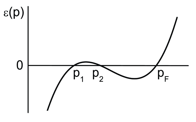
Figure 1: Location of roots of the equation $\epsilon(p,T=0)=0$ measured from the chemical potential $\mu$ beyond the bifurcation point

In ordinary (“canonical”) Fermi liquids, there exists a one-to-one correspondence between the single-particle spectrum $\epsilon(p)$ and the momentum $p$, at least in the vicinity of the Fermi surface. This is equivalent to asserting that the equation

$${p^{2}\over 2M}+\Sigma(p,\varepsilon=0)=\mu\$$ (19)

has a single solution $p=p_{F}$, since the group velocity $v_{F}$ is positive. Within FL theory, Eq. (19) reduces to the relation

$$\epsilon(p,T=0;n_{F})=0\ ,$$ (20)

where the energy $\epsilon(p)$, measured from the chemical potential $\mu$, is evaluated with the Landau quasiparticle momentum distribution $n_{F}(p)=\theta(p-p_{F})$. However, it is a key ingredient of the topological scenario for the QCP that at a critical value of some input parameter, specifically the density $\rho_{\infty}$ or a coupling constant $g_{\infty}$, the group velocity $v_{F}$ vanishes. (This feature in demonstrated in several numerical examples presented in Sec. V.)

Beyond the critical point, e.g. at $g>g_{\infty}$, Eq. (20) acquires at least two new roots (see Fig. 1), triggering a topological phase transition.volrev Significantly, terms proportional to $\epsilon\ln\epsilon$, which are present in the mass operator $\Sigma$ of marginal Fermi liquids, do not enter Eqs. (19) and (20).

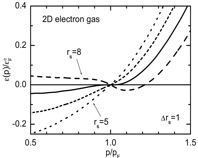
Figure 2: Single-particle spectrum $\epsilon(p,T=0)$ of a homogeneous 2D electron gas, measured from the chemical potential $\mu$, in units of $\varepsilon_{F}^{0}=p^{2}_{F}/2M$, evaluated microscopically bz at $T=0$ for different values of the dimensionless parameter $r_{s}=\sqrt{2}Me^{2}/p_{F}$.

The bifurcation point $p_{b}$ of these equations can emerge anywhere in momentum space. Here we examine the case in which $p_{b}$ coincides with the Fermi momentum $p_{F}$, so that at the critical density $\rho_{\infty}$, the group velocity $v_{F}(\rho_{\infty})$ changes its sign. This distinctive feature of the topological scenario for the QCP is in agreement with results of microscopic calculations of the single-particle spectrum $\epsilon(p,T=0)$ of 2D electron gas,bz as illustrated in Fig. 2. It is seen that the sign of $v_{F}$ remains positive until the dimensionless parameter $r_{s}$ attains a critical value $r_{\infty}\simeq 7.0$, where $v_{F}$ vanishes. At larger $r_{s}$, the group velocity $v_{F}=\left(d\epsilon(p,n_{F})/dp\right)_{0}$, evaluated with the quasiparticle momentum distribution $n_{F}(p)$, is negative. Having lost it stability, the Landau state is replaced by a new state through the intervention of a topological phase transition.

A qualitatively similar situation is to be expected in anisotropic Fermi systems. In support of this statement, we may refer to the first example of the QCP, namely the Lifshitz saddle point,lifshitz which is characterized by a density of states diverging at $T\to 0$ as $N(T,\rho_{\infty})\sim\ln(1/T)$. This example has been elaborated specifically for anisotropic 2D electron systems in solids. Close to the saddle point, the QCP single-particle spectrum has the form $\epsilon({\bf p},\rho_{\infty})=(1/2)(p^{2}_{x}/M_{xx}-p^{2}_{y}/M_{yy})$, with the components $p_{x}$ and $p_{y}$ specifying the distance to the saddle point in momentum space. In the Lifshitz model, the quantities $M_{xx}$ and $M_{yy}$ have comparable finite values. If one of these parameters, say $M_{xx}$, becomes much larger than $M_{yy}$, we arrive at the so-called extended saddle point, which has been considered in connection with high-$T_{c}$ superconductivity in Ref. abr, . The corresponding phase transition, associated with the divergence of $M_{xx}$, is also topological.

III Poincaré mapping for strongly correlated Fermi systems

In this section we restrict considerations to homogeneous matter at zero temperature. Microscopic calculations of the single-particle spectrum $\epsilon(p,T=0)$ are as yet available only for several simple types of bare interactions between particles. Moreover, there is no microscopic theory beyond the point where the Landau state loses its stability. On the other hand, given a phenomenological interaction function $f$, Eq. (5) holds on both the sides of the topological QCP, since the $z$-factor retains a nonzero value. Numerical iteration is a standard approach to solution of an equation such as Eq. (5). We shall see that the mathematical counterpart of iteration, Poincaré mapping, which has been widely exploited in theory of turbulence,lanh is also instrumental in elucidating the striking features inherent in solutions of Eq. (5) beyond the QCP.

The discrete iterative map corresponding to Eq. (5) reads

$${\partial\epsilon^{(j+1)}(p)\over\partial p}={p\over M}+{1\over 3\pi^{2}}\int f_{1}(p,p_{1}){\partial n^{(j)}(p_{1})\over\partial p_{1}}p^{2}_{1}dp_{1}\ ,$$ (21)

the iterate $\mu^{(j+1)}$ for the chemical potential being determined from the normalization condition (2). The index $j=0,1,2,\ldots$ counts the iterations (zeroth, first, second, $\ldots$). The iterate $n^{(j+1)}(p)$ of the momentum distribution $n(p)$ is generated by inserting the corresponding spectral iterate $\epsilon^{(j+1)}(p)$ into Eq. (4), which at $T=0$ reduces to a Heaviside function $n(p)=\theta(-\epsilon(p))$.

III.1 Poincaré mapping for systems with a nonsingular interaction

The key quantity of the Poincaré analysis in the Fermi liquid problem is the group velocity

$${d\epsilon^{(1)}(p)\over dp}={p\over M}-{p^{2}_{F}\over 3\pi^{2}}f_{1}(p,p_{F};\rho)\ ,$$ (22)

evaluated by inserting the standard FL momentum distribution $n_{F}(p)=\theta(p-p_{F})$ into the right-hand side of Eq. (21) as the zero iterate (starting approximant) for the quasiparticle momentum distribution $n(p)$. In canonical Fermi liquids, for which the sign of $v_{F}$ is positive and the function $\epsilon^{(1)}(p)$ has the single zero at $p=p_{F}$, the first iterate $n^{(1)}(p)$ and all higher iterates for the distribution $n(p)$ coincide with the $n_{F}(p)$, this being a fixed point of the transformation. However, beyond the QCP the sign of the group velocity $v_{F}$ evaluated from Eq. (22) becomes negative, and the first iterate $\epsilon^{(1)}(p)\equiv\epsilon(p;n_{F})$ for the spectrum already has three zeroes $p_{1}^{(1)}<p_{2}^{(1)}<p_{3}^{(1)}$, implying three kinks in the momentum distribution.

At the second step, the evolution of the iteration process follows different patterns, depending on the presence or absence of a long-range component in the effective interaction between quasiparticles (long range in coordinate space). We first consider the simpler case in which the effective interaction $f(k)$, local in coordinate space, has no singularities. In this case the interaction function $f_{1}(p,p_{F})$ can then expanded in a Taylor series in the variable $p-p_{F}$, and Eq. (5) may be recast as a set of algebraic equations. Then, as the straightforward analysis demonstrates and the numerical calculations described in Sect. V confirm, the shape

$$\epsilon(p,T=0)\sim(p-p_{1})(p-p_{2})(p-p_{3})$$ (23)

of the spectrum remains the same independently of the number of iterations, with three roots $p_{1}<p_{2}<p_{3}$ specifying the location of the three sheets of the Fermi surface and lying close to the QCP Fermi momentum $p_{\infty}$. Correspondingly, the spectrum $\epsilon(p,T=0)$ changes smoothly in the momentum regimes removed from the kinks, but oscillates in the interval $[p_{1},p_{3}]$. The amplitude of the oscillation, i.e., the maximum value

$$T_{m}=\max|\epsilon(p,T=0)|\ ,\quad p_{1}<p<p_{3}\,,$$ (24)

of the departure of $|\epsilon(p,T=0)|$ from 0, defines a new energy scale of the problem: if temperature $T$ attains values comparable to $T_{m}$, the kink structure associated with the multi-connected Fermi surface is destroyed.

To evaluate $T_{m}$, we note that according to Eq. (23) the group velocity $d\epsilon(p)/dp$ is a parabolic function of $p$, conveniently written as

$${d\epsilon(p)\over dp}=-X+Y(p-p_{m})^{2}\ ,$$ (25)

where $p_{m}$ determines the location of the minimum of the group velocity. Comparison of Eqs. (23) and (25) leads to the following set of equations,

$$r_{1}+r_{2}+r_{3} = 0\ ,$$

$$r_{1}r_{2}+r_{1}r_{3}+r_{2}r_{3} = -{3X\over Y}\ ,$$

$$(p_{m}+r_{1})^{3}-(p_{m}+r_{2})^{3}+(p_{m}+r_{3})^{3} = 3\pi^{2}\rho\ ,$$ (26)

for the three (shifted) roots $r_{k}=p_{k}-p_{m}$, with $k=1,2,3$. The last of Eqs. (26) is obtained from the normalization condition (2).

In the vicinity of the QCP where $X=X_{\infty}=0$, the parameter $p_{m}$ and the positive quantities $X(\rho)$ and $Y(\rho)$ can be shown to change linearly with $\rho-\rho_{\infty}$. Simple but lengthy algebra then yields

$$r_{3}\simeq-r_{1}\sim|\rho-\rho_{\infty}|^{1/2}\,,\quad r_{2}\sim|\rho-\rho_{\infty}|\ .$$ (27)

These results allow us to express relevant parameters in terms of the difference $\rho-\rho_{\infty}$, namely (i) $\Delta p=p_{3}-p_{1}$, which characterizes the range of the flattening of the spectrum $\epsilon(p,T=0)$ beyond the QCP, (ii) the temperature $T_{m}$ associated with the crossover from standard FL behavior to NFL behavior, and (iii) the zero-temperature density of states $N(0)\sim\sum_{k}[d\epsilon(p=p_{k})/dp]^{-1}$, which replaces the ratio $M^{*}/M$ in the standard FL formulas for the specific heat, spin susceptibility, etc. We find

$$\Delta p\sim|\rho-\rho_{\infty}|^{1/2},\;T_{m}\sim|\rho-\rho_{\infty}|^{3/2},\;N(0)\sim|\rho-\rho_{\infty}|^{-1}\ .$$ (28)

To our knowledge, the multi-connected Fermi surface, shown here to arise in the homogeneous case, was first considered in 1950 by Fröhlich.frohlich Within the Hartree-Fock (HF) approach, model variational calculations for the ground-state energies of homogeneous systems leading to a multi-connected Fermi surface were performed more than 20 years ago,Vary while the corresponding phase transition was first discussed in terms of HF single-particle spectra in Ref. baym, and later in Ref. schofield, . The original calculations of properties of this transition on the basis of Eq. (5) were performed in Refs. zb, ; shagp, . These calculations show that as the coupling constant moves away from the QCP value $g_{\infty}$, the number of sheets of the Fermi surface, which coincides with the number of the roots of Eq. (20), grows very rapidly, with the distance between the sheets shrinking apace. Importantly, in all these solutions, the relation

$$n^{2}(p)=n(p)\ ,$$ (29)

inherent in the standard FL picture, is still obeyed.

III.2 2-cycles in Poincaré mapping for systems with a singular interaction function $f$

A remarkable feature of equations relevant to the turbulence problem is the doubling of periods of motion, giving rise to dynamical chaos.feig ; lanh If now the nonlinear system corresponding to Eq. (21) is considered within this context by associating an iteration step with a step in time, one’s first instinct is to assert that such a phenomenon cannot occur when Poincaré mapping is implemented, since chaos in the classical sense cannot play a role in the ground states of Fermi liquids at $T=0$. And indeed, this general assertion seems to be validated by the results of the preceding subsection. However, the Taylor expansion of the interaction function $f_{1}(p,p_{F})$ that we employed in the above analysis fails in the case of long-range effective interactions. The Fourier transform $f(k\to 0)$ becomes singular, and the previous analysis is inapplicable.

As an interesting example, we note that such a singularity exists in the bare interaction

$$\Gamma^{0}({\bf p}_{1},{\bf p}_{2},{\bf k},\omega=0)=-g{{\bf p}_{1}\cdot{\bf p}_{2}-({\bf p}_{1}\cdot{\bf k})({\bf p}_{2}\cdot{\bf k})/k^{2}\over k^{2}}$$ (30)

between quarks in dense quark-gluon plasma, wherein $g>0$.

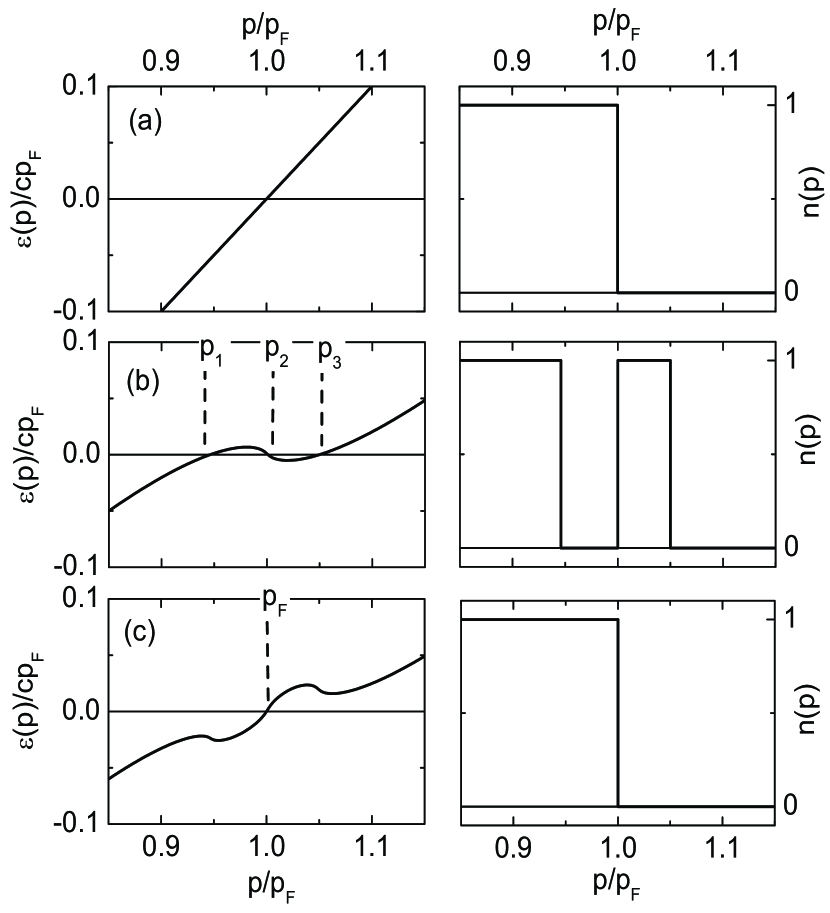
Figure 3: Iterative maps for the quark-gluon plasma problem (31) with the bare spectrum $\epsilon_{p}^{0}=cp$ and the dimensionless parameter $\alpha=g/c=0.3$. Left panels: spectral iterates $\epsilon^{(j)}(p)$ with $j=0,1,2$, in units of $cp_{F}$. Right panels: momentum-distribution iterates $n^{(j)}(p)$. The 2-cycle reveals itself in the coincidence between the first and third right panels.

In this example, Eq. (5) has the formbaym

$${\partial\epsilon(p)\over\partial p}={\partial\epsilon^{0}_{p}\over\partial p}+g\int\ln{2p_{F}\over p-p_{1}}{\partial n(p_{1})\over\partial p_{1}}dp_{1}\ ,$$ (31)

where $\epsilon^{0}_{p}\simeq cp$ is the bare single-particle spectrum of light quarks.

The first iterate for the spectrum, evaluated from Eq. (31) with the distribution $n_{F}(p)$, has an infinite negative derivative $d\epsilon^{(1)}/dp$ at the Fermi surface. It then follows that independently of the value of the dimensionless coupling constant $\alpha=g({\partial\epsilon^{0}_{p}/\partial p})^{-1}_{0}$, Eq. (20), with $x=p/p_{F}-1$, takes the form

$$x\left(1-\alpha\ln{2\over x}\right)=0\ ,$$ (32)

and has three different roots $-x_{0}$, $0$, and $x_{0}$, with $x_{0}=2\exp^{-1/\alpha}$. The corresponding first iterate of the momentum distribution is $n^{(1)}(p)=\theta(x+x_{0})-\theta(x)+\theta(x-x_{0})$. The next iteration step yields $n^{(2)}(p)\equiv n_{F}(p)$, so the standard FL structure of the momentum distribution is recovered. The nonlinear system enters a 2-cycle that is repeated indefinitely; one is dealing with a 2-cycle Poincaré mapping.

The first two iterations of the mapping process are illustrated in Fig. 3. The top-left panel of this figure shows the bare spectrum $\epsilon^{(0)}(p)\equiv\epsilon^{0}(p)$. The first iterate of the spectrum, $\epsilon^{(1)}(p)$, appearing in the middle-left panel, is evaluated by folding the kernel $\ln(2p_{F}/(p-p_{1}))$ with the Fermi-step $n_{F}(p)$, shown in the top-right panel. The spectrum $\epsilon^{(1)}(p)$ possesses three zeroes: $p_{1}<p_{F}$, $p_{2}=p_{F}$, and $p_{3}>p_{F}$, implying that the first iterate $n^{(1)}(p)$, drawn in middle-right panel, describes a Fermi surface with three sheets. This distribution differs from the ordinary Fermi step only in the momentum interval $-x_{0}<x<x_{0}$. The next iterate, $\epsilon^{(2)}(p)$ (bottom-left panel), again has a single zero $p_{F}$, and the corresponding momentum distribution $n^{(2)}(p)$ (bottom-right panel) coincides identically with $n_{F}(p)$.

A 2-cycle Poincaré mapping also arises in treating the Nozières model,noz for which the interaction function $f$ has the limited singular form $f({\bf q})=g\delta({\bf q})$ with $g>0$. In this model, the iterative maps (illustrated in Fig. 4) are generated from the equation

$$\epsilon^{(j+1)}(p)+\mu^{(j+1)}=p^{2}/2M+gn^{(j)}(p)\ ,$$ (33)

along with the normalization condition (2) for $n^{(j+1)}(p)=\theta(-\epsilon^{(j+1)}(p))$. Here, the odd iterates $n^{(2j+1)}(p)$ of the momentum distribution deviate from the $n_{F}(p)$ in the interval $-g/4\varepsilon^{0}_{F}<x<g/4\varepsilon^{0}_{F}$, but in even iterations, the Fermi step reappears intact.

Numerical analysis demonstrates that similar 2-cycles arise when Poincaré mapping based on Eq. (21) is implemented for other systems having an interaction function that is singular at $k\to 0$ (see Sec. V). In all these cases, the emergence of a 2-cycle turns out to be an unambiguous signal of the instability of the standard Landau state. Moreover, the domain of momentum involved in the cyclic behavior is almost identical with the domain within which an improved iteration algorithm fails to converge (see Sec. III.D). As will be seen, this concurrence is significant in that the associated volume of momentum space provides a measure of the entropy stored in the exceptional ground state that replaces the Landau state.

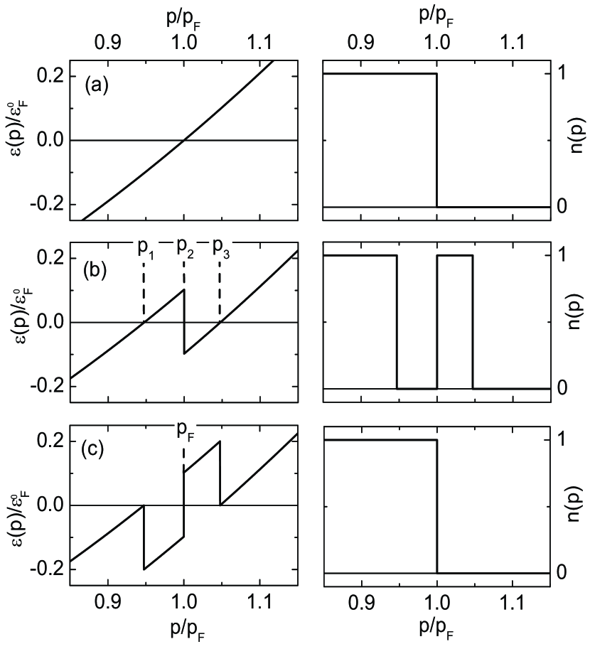
Figure 4: Same as in Fig. 3 for the discretized Nozières model (33) with $g=0.2\varepsilon_{F}^{0}$.

III.3 2-cycles in Poincaré mapping for finite systems

In finite Fermi systems—nuclei, atoms, atomic clusters, quantum dots, molecules, $\ldots$—integration over momenta in Eq. (21) is replaced by summation over single-particle quantum numbers. As a concrete illustration, let us explore a schematic modeltwolevel of a spherical nucleus, in which the single-(quasi)particle energies are independent of the magnetic quantum number $m$. We consider two neutron levels available for filling in an open shell, denoted $0$ and $+$.

In the presence of a quasiparticle interaction $f$, the energies of the two levels are influenced when neutrons are added to the system. With this in mind, the energies of levels $0$ and $+$ when $N$ neutrons are added to level $0$ and none added to level $+$ are denoted $\epsilon_{0}(N,0)\equiv\epsilon_{0}(N)$ and $\epsilon_{+}(N,0)\equiv\epsilon_{+}(N)$, respectively. The initial distance between the two levels, with no added neutrons, is $D(0,0)=\epsilon_{+}(0,0)-\epsilon_{0}(0,0)=D_{0}>0$, having designated $0$ as the lower of the two levels. The behavior of the level distance $D(N,0)=\epsilon_{+}(N,0)-\epsilon_{0}(N,0)$ as neutrons are added is crucial to the behavior of the system. To facilitate the argument, we adopt a highly simplified interaction between neutrons, retaining in $f$ only a principalmigdal ; ring $\delta({\bf r})$-like component. Also for simplicity, the relevant matrix elements for determining the energy shifts are reduced to two, namely $f_{00}=f_{++}$ and $f_{0+}=f_{+0}$, which (with $k=0,+$) are calculated as

$$f_{kk^{\prime}}=\int R_{k}^{2}(r)f\left(\rho(r)\right)R_{k^{\prime}}^{2}(r){r^{2}dr\over 4\pi}$$ (34)

in terms of the radial parts of the corresponding single-particle wave functions. We then have

$$\epsilon_{0}(N)=\epsilon_{0}+Nf_{00},\quad\epsilon_{+}(N)=\epsilon_{0}+D_{0}+Nf_{+0}\ ,$$ (35)

so that the distance $D(N,0)$ varies as

$$D(N,0)=D_{0}+N\left(f_{+0}-f_{00}\right)\ .$$ (36)

Significantly, in both the atomic and nuclear problems, the sign of the difference $f_{0+}-f_{00}$ is negative,twolevel so that the function $D(N,0)$ falls off as the number $N$ of added neutrons increases. The standard FL scenario, in which all added quasiparticles occupy the level $0$, remains valid as long as the level distance $D(N,0)$ remains positive. As seen from Eq. (36), this distance changes sign when $N$ reaches the critical number $N_{c}=D_{0}/(f_{00}-f_{+0})$. Thus, at $N>N_{c}$,

$$D(N,0)=(N-N_{c})\left(f_{+0}-f_{00}\right)<0\ ,$$ (37)

forcing all the quasiparticles to resettle into the level $+$.

To perform the next iteration, one calculates the distance $D(0,N)\equiv\epsilon_{0}(0,N)-\epsilon_{+}(0,N)$ between levels $0$ and $+$ for the case that all the quasiparticles occupy level $+$, obtaining

$$D(0,N)=D_{0}+N\left(f_{+0}-f_{++}\right)\simeq-(N-N_{c})\left(f_{00}-f_{+0}\right)\ .$$ (38)

Since $N$ exceeds the critical number $N_{c}$, the sign of this quantity is negative. This implies that the priority for filling reverses again, requiring that all the quasiparticles return to the level $0$. This 2-cycle is repeated indefinitely.

In the weak coupling limit where $f_{00}\to 0$, the critical number $N_{c}$ diverges, and filling of the level $0$ is completed before $N$ reaches $N_{c}$. In this case, level-filling occurs normally, the 2-cycle being unattainable. However, in the atomic problem, the magnitude of the matrix elements of the Coulomb interaction between the orbiting electrons significantly exceeds the distance between neighboring single-particle levels. As a consequence, 2-cycles emerge at $N\simeq 1$ in the iterative maps for atoms of almost all elements not belonging to the principal groups. The implication is that the electronic systems of these elements do not obey standard FL theory. The same conclusion is valid for many heavy atomic nuclei with open shells.

Naturally, the occurrence of such 2-cycles in the analysis of level-filling in finite Fermi systems presents a dilemma that must be resolved. Here (and in the other examples) such cyclic behavior is obviously unphysical. Here the resolution lies in the merging of single-particle levels and their partial occupation, hence in behavior that conflicts with standard FL theory yet in fact maintains consistency within the broader framework of Landau theory.twolevel

III.4 Modified Poincaré mapping and new insight from chaos theory

Apparently, the occurrence of persistent 2-cycles in the iterative maps of Eq. (21) prevents us from finding true solutions of the fundamental Landau equation (5) beyond the QCP for a specific class of Fermi systems possessing singular effective interactions. It can be argued, however, that this failure is a consequence of the inadequacy of the iterative procedure employed, which works perfectly on the FL side of the QCP. Indeed, a refined procedure that mixes iterations does allow one to avoid the emergence of these 2-cycles. Nevertheless, the improved procedure possesses the same feature: the iterations do not converge, although the pattern of their evolution becomes more complicated and—as will be seen—both intriguing and suggestive.

Figure 5: Iterative maps for the discretized Nozières model (39) when inputs taken from the two preceding iterations are mixed with the parameter $\zeta=0.2$. Left panels: spectra $\epsilon^{(j)}(p)$ with $j=0,1,2,3$, in units of $\varepsilon^{0}_{F}$. Right panels: momentum distributions $n^{(j)}(p)$.

By way of illustration let us consider a modified Poincaré mapping for the Nozières model, again with coupling constant $g=0.2\varepsilon^{0}_{F}$. Choosing a mixing parameter $\zeta$, the equation

$$\epsilon^{(j+1)}(p)+\mu^{(j+1)}=(1-\zeta)\,[\epsilon^{(j)}(p)+\mu^{(j)}]$$ (39)

$$+\zeta\,[p^{2}/2M+gn^{(j)}(p)]\qquad\qquad$$

is used to generate the iterative maps shown in Fig. 5. Recovery of the ordinary Fermi distribution $n_{F}(p)$, an inherent feature of the standard iteration procedure at the second iteration (see Fig. 4), no longer occurs; indeed, the sequence of iterations fails to converge, even to a limit cycle. The number of sheets remains three at the second iteration. At the third, however, seven sheets of the Fermi surface emerge, and the number of sheets continues to increase in successive iterations. At the same time, the distance between the sheets continues to narrow, since the domain of momentum space in which the improved iteration procedure does not converge remains almost the same as that in which the standard procedure finds a 2-cycle. This phenomenon of proliferating Fermi sheets recapitulates a scenario envisioned in the seminal study by Pethick et al.baym of the quark-gluon plasma based on the interaction function (30).

Treating the number $j=1,2,3,\ldots$ of the iteration as a discrete time step, the sequence of the pictures in the left column of Fig. 5 shows the “temporal” evolution of the quasiparticle spectrum. At any time-step $t$, the single-particle energy $\epsilon(p,t)$ falls off steadily as $p$ goes to zero, while its sign changes unpredictably in a finite region $\Omega_{t}$ of momentum space adjacent to the Fermi surface. These erratic changes of sign induce unpredictable jumps of the occupation numbers $n(p,t)$ between the two values 0 and 1. Significantly, at $T=0$ and as $t$ goes to infinity, the region of momentum space in which iterations of Eq. (5) fail to converge tends to a definite limit $\Omega$. The lack of convergence of the iteration process may be attributed to the presence of a kind of “quantum chaos.” Since entropy is a natural byproduct of chaos, we tentatively identify $2\Omega\ln 2$ as its measure in the present context, where $\Omega$ now denotes the numerical volume, in momentum space, of the domain of non-convergence, and the factor 2 comes from the two spin projections. Thus, $2\Omega\ln 2$ is interpreted as a special entropy associated with a Fermi system for which iteration of Eq. (5) does not converge to a solution.

This naive formula for the special entropy can be refined. To do so, we introduce a “time-averaged” single-particle energy ${\overline{\epsilon}}(p)$ by appropriating a standard formula from statistical physics,

$${\overline{\epsilon}}(p)=\lim\limits_{T\to\infty}{1\over T}\int\limits_{0}^{T}\epsilon(p,t)dt\equiv\lim\limits_{N\to\infty}{1\over N}\sum\limits_{0}^{N}\epsilon^{(j)}(p)\ ,$$ (40)

in which the iterates for $\epsilon(p)$ are averaged over the fictitious time $t$. In the same way, we introduce a corresponding time average ${\overline{n}}(p)$ of the iterates of the momentum distribution $n(p)$. The relation between the two time averages, simply

$${\overline{\epsilon}}(p)=p^{2}/2M-\mu+g{\overline{n}}(p)\ ,$$ (41)

stems from Eq. (33). Remarkably, the mixing parameter $\zeta$ cancels out in arriving at this relation.

Obviously, ${\overline{n}}(p)$ only takes values 0 or 1 wherever the iterations converge, and then ${\overline{\epsilon}}(p)$ is a parabolic function of $p$ coinciding with the true single-particle energy. However, as seen from Eq. (40) and verified by results shown in the left column of Fig. 5, the function ${\overline{\epsilon}}(p)$ vanishes identically in the domain $\Omega$ where iterations fail to converge, yielding

$$n_{*}(p)={\mu-p^{2}/2M\over g}\ ,\quad{\bf p}\in\Omega\ .$$ (42)

The notation $n_{*}(p)$ has been introduced to signify a smoothed momentum distribution, determined by averaging iterates $\epsilon(p,t)$ for the single-particle energy according to the prescription (40).

Thus, by implementing (i) a modified Poincaré mapping procedure based on Eq. (39) together with (ii) “time-averaging” of iterates for $\epsilon(p)$ and $n(p)$ in the manner of Eq. (40), we have found a solution of the problem that satisfies the Pauli principle in the domain $\Omega$ where the sequence of iterates does not converge. The solution so obtained is independent of the parameters specifying the refined iteration procedure. The boundaries $p_{i}$ and $p_{f}$ of the momentum interval $p_{i}<p_{F}<p_{f}$ defining the domain of non-convergence are determined by the conditions $n_{*}(p_{i})=1$ and $n_{*}(p_{f})=0$. Thus, the quasiparticle momentum distribution $n(p)$ corresponding to the new solution, hereafter written as $n_{*}(p)$, is given by 1 and 0, respectively, at $p\leq p_{i}$ and $p\geq p_{f}$, and by Eq. (42) in between.

Now we are prepared to introduce a Kolmogorov-like entropy

$$S_{*}=-2\int[n_{*}(p)\ln n_{*}(p)+(1-n_{*}(p))\ln(1-n_{*}(p))]d\upsilon\ ,$$ (43)

in which the second term of the integrand accounts for the equal status of particles and holes. According to the definition of $n_{*}(p)$, the integrand in Eq. (43) vanishes outside the domain $\Omega$, and we see that $S_{*}$ is essentially proportional to the volume of this domain (also called $\Omega$). Setting $n_{*}(p)$ inside $\Omega$ equal to a typical value 1/2, one does indeed arrive at $S_{*}=2\Omega\ln 2$.

This program is to be implemented similarly when dealing with other Fermi systems for which iteration of Eq. (5) does not converge to a solution. The first step is to integrate Eq. (5) and find an explicit relation connecting the spectrum $\epsilon(p)$ with the momentum distribution $n(p)$. The average quantity ${\overline{\epsilon}}(p)$ is then constructed by means of Eq. (40). Since this quantity vanishes identically in the domain $\Omega$ where iteration fails to converge, we obtain a closed equation

$${\overline{\epsilon}}(p,n_{*})=0\ ,\quad{\bf p}\in\Omega\,,$$ (44)

for finding the smoothed, NFL component of the momentum distribution $n_{*}(p)$ and calculating the entropy $S_{*}$.

The possibility of a nonzero value of the entropy at $T=0$ beyond the QCP is an inherent feature of the topological scenario being explored within the original Landau framework. The existence of such an entropy excess for a system whose interaction function $f$ has a long-range component means that the associated ground state is statistically degenerate.lanl These findings offer a new perspective not only on the QCP itself, but also on the concept of “quantum chaos”—suggesting a novel role for the phenomenon of chaos in quantum many-body systems. The underlying connections and their implications will be developed in depth in a separate paper.

IV Fermion condensation as a species of topological phase transition

An equation identical to (44) can be derived in another way,ks based on the premiselan that the ground-state energy $E$ of the system is a functional of the quasiparticle momentum distribution $n(p)$. For canonical Fermi liquids, the minimum of $E[n]$ is attained at the boundary point $n_{F}(p)=\theta(p-p_{F})$ of the manifold $\{n\}$ containing all candidates for the function $n(p)$ that satisfy the Pauli restriction $0\leq n\leq 1$ and particle-number conservation. In Ref. ks, , the minimum of the model functional

$$E=\int{p^{2}\over 2M}n({\bf p})\,d\upsilon+{f\over 2}\int{n({\bf p}_{1})n({\bf p}_{2})\over|{\bf p}_{1}-{\bf p}_{2}|}\,d\upsilon_{1}\,d\upsilon_{2}$$ (45)

was found. The Fermi step $n_{F}(p)$ turns out to be the true ground-state quasiparticle momentum distribution only if correlations are rather weak. Otherwise a topological phase transition occurs at some critical coupling constant $f_{c}$. At $f>f_{c}$, a new distribution is determined from the variational conditionks

$${\delta E\over\delta n({\bf p})}=\mu\ ,\quad{\bf p}\in\Omega\ .$$ (46)

For the above model functional, this condition takes the explicit form

$${p^{2}\over 2M}+f\int{n({\bf p}_{1})\over|{\bf p}_{1}-{\bf p}|}d\upsilon_{1}=\mu\ ,\quad{\bf p}\in\Omega\ .$$ (47)

This equation is easily solved for $n(p)$ by exploiting a transparent analogy with a system of charged particles moving in an external elastic field. The result, yielding $n_{*}(p)={\rm const.}<1$ at $p<p_{f}$ and $n_{*}(p)=0$ otherwise, is drastically different from the familiar FL solution. Importantly, the same result is obtained when the iteration/averaging procedure established in Sec. III.D is applied to Eq. (47). For the Nozières modelnoz studied in Subsec. III.D, Eq. (46) may also be solved analytically, and the solution is again in agreement with the result (42) of the procedure introduced there.

Prior to discussing this coincidence in more detail, let us focus on Eq. (46) itself. This variational condition, studied rather extensively during the last decade,ks ; vol ; noz ; physrep ; khv ; schuck ; normfc ; kzphysb ; ikk ; kzc2005 ; yak ; shagrev is generic. To illuminate its nature and conceptual status, we invoke a mathematical correspondence of the functional $E[n(p)]$ with the energy functional $E[\rho(r)]$ of statistical physics. If the interactions are weak, the latter functional attains its minimum value at a density $\rho$ determined by the size of the vessel that contains it, and which it fills uniformly. In such cases, solutions of the variational problem evidently describe gases. On the other hand, if the interactions between the particles are sufficiently strong, there arise nontrivial solutions of the variational condition

$${\delta E[\rho]\over\delta\rho(r)}=\mu$$ (48)

that describe liquids, whose density is practically independent of boundary conditions.

The energy functional $E[n]$ of our quantum many-body problem must have two analogous types of solutions, with an essential difference: solutions $n_{*}(p)$ of the variational condition (46) must satisfy the condition $0\leq n(p)\leq 1$. This condition cannot be met in weakly correlated Fermi systems, but it can be satisfied in systems with sufficiently strong correlations.

Turning now to the coincidence between solutions of Eq. (46) and Eq. (44), we note that the quasiparticle energy is by definition just the derivative of the ground state $E$ with respect to the quasiparticle momentum distribution $n(p)$, or, referred to the chemical potential, just $\epsilon(p)=\delta E/\delta n(p)-\mu$. Consequently, the variational condition (46) may recast as an equation

$$\epsilon(p,n_{*})=0\ ,\qquad{\bf p}\in\Omega\,,$$ (49)

that is in fact identical to Eq. (44). This equivalence allows us to use the same notation $n_{*}$ for the NFL momentum distribution $n(p)$ in the two formulations of the problem.

The above analysis and discussion make it clear that the most salient of the unorthodox features we have uncovered in applying the original Landau quasiparticle formalism to the behavior of strongly correlated Fermi systems beyond the QCP is that at $T=0$ the single-particle spectrum $\epsilon(p)$ becomes completely flat over a finite domain $\Omega$ of momenta adjacent to the Fermi surface. One may envision this phenomenon as a swelling of the Fermi surface. Another generic feature, concomitant with flattening of the single-particle spectrum, is partial occupation of single-particle states of given spin, i.e., $n(p)$ is no longer restricted to the values 0 and 1, but may take any value in the interval $[0,1]$.

This extraordinary behavior is associated with a topological phase transition fundamentally different from the one which features a proliferating number of sheets of the Fermi surface, in that the roots of the equation $\epsilon(p)=0$ now form a continuum instead of a countable set. Since the Landau quasiparticles experience no damping, the single-quasiparticle Green function becomes

$$G(p,\varepsilon)={1-n_{*}(p)\over\varepsilon{+}i\delta}+{n_{*}(p)\over\varepsilon{-}i\delta}\,,\quad\ {\bf p}\in\Omega\,,$$ (50)

in the domain $\Omega$ of vanishing $\epsilon(p,n)$ and retains its FL form for $p$ outside $\Omega$. This particular structure of the Green function (50) may be characterized by a topological charge defined as the integral vol ; volrev

$${\cal N}=\int\limits_{\gamma}G(p,\xi)\,\partial_{l}G(p,\xi){dl\over 2\pi i}\ ,$$ (51)

where the Green function is considered on the imaginary axis of energy $\varepsilon=i\xi$ and the integration is performed over a contour in $({\bf p},\xi)$-space that embraces the Fermi surface. For canonical Fermi liquids and systems with a multi-connected Fermi surface, the topological charge ${\cal N}$ is an integer, whereas for the more exotic states characterized by a completely flat portion of the spectrum $\epsilon(p)$, its value is half-odd-integral.vol ; volrev

Aided by the variational condition (46), one can elucidate what happens when a quasiparticle with momentum ${\bf p}\in\Omega$ is added to the system, assumed again to be homogeneous. In contrast to what happens with a canonical Fermi liquid, the addition of just one quasiparticle now induces a rearrangement of the whole distribution function $n_{*}(p)$. This implies that the kind of system being considered cannot be treated as a gas of interacting quasiparticles, even though the original Landau quasiparticle concept still applies.

The set of states for which Eq. (49) [or Eq.(53)] is satisfied has been called the fermion condensate (FC),ks while the topological phase transition in which the Fermi surface swells from a line to a surface in 2D, or from a surface to a volume in 3D, is otherwise known as fermion condensation. In finite systems the phenomenon of fermion condensation exhibits itself as merging of neighboring single-particle levels.twolevel Unfortunately, the terms fermion condensation and fermion condensate have unnecessarily promoted controversy. Theorists are condition to think that in contrast to bosons, fermions cannot condense, because fermions cannot occupy the same quantum state. However, in everyday life, “condensation” means simply a dramatic increase of density. For example, people use the word to describe what occurs when the vapor in clouds forms into liquid drops that fall as rain. On the other hand, statistical physics deals with occupation numbers rather than with wave functions, and the thermodynamic properties of a Bose gas at low temperatures are properly evaluated by treating Bose condensation as a process in which a macroscopic number of bosons occupy the same zero-momentum single particle state, all with single-particle energy equal to the chemical potential $\mu$.

Ideally, in experimental measurements of neutron scattering on liquid ⁴He, Bose condensation is reflected in a sharp peak in the density of states $\rho(\epsilon)=\rho_{c}\delta(\epsilon)$, with a prefactor $\rho_{c}$ that is to be interpreted as the density of the Bose condensate. In strongly correlated Fermi systems, fermions are also capable of condensation in much the same sense: a macroscopic number can have the same energy $\mu$. If so, it follows from Eq. (50) that the zero-temperature density of states, which is associated with the integral of the imaginary part of the retarded Green function $G_{R}(p,\epsilon)$ over momentum space, has the same kind of peak $\rho(\epsilon)=\rho_{c}\delta(\epsilon)$, where $\rho_{c}$ is the now the FC density. We hasten to add that although a macroscopic number of fermions have the same energy, they possess different momenta; hence the existence of states containing a FC does not contradict the Pauli exclusion principle.

In spite of the similarities between boson and fermion condensation, an important difference between the structure functions describing them must be noted. In the Bose case, a macroscopic number of particles reside in condensate for all temperatures lower than the critical temperature, with all the bosons having zero momentum and energy $\epsilon(p)=0$. On the other hand, in the Fermi case, any elevation of the temperature from zero acts to lift the degeneracy of the single-particle spectrum in the domain $\Omega$. Indeed, since a minute temperature elevation does not affect the FC momentum distribution, Eq. (4) can be inverted to yield noz

$$\epsilon(p,T\to 0)=T\ln{1-n_{*}(p)\over n_{*}(p)}\ ,\qquad{\bf p}\in\Omega\ .$$ (52)

Thus, the dispersion of the single-particle spectrum of systems having a FC turns out to be proportional to temperature, in contrast to the situation for canonical Fermi liquids, where it is independent of $T$. This distinction can be employed for unambiguous delineation of the boundaries of the domain $\Omega$ occupied by the FC at finite $T$.

In nonhomogeneous systems, finite or infinitely extended, appropriate single-particle states are no longer eigenstates of momentum ${\bf p}$, so Eq. (49) must be replaced by

$$\epsilon_{\lambda}=0\ ,\quad\lambda\in\Omega\ ,$$ (53)

where $\lambda$ is set of quantum numbers specifying the single-particle state. At finite temperatures, the FC degeneracy is lifted according to the same formula (52) as for the homogeneous case.

V Numerical calculations

Figure 6: Single-particle spectrum $\epsilon(p)$ (top panels) and derivative $d\epsilon(p)/dp$ in units of $v_{F}^{0}=p_{F}/M$ (bottom panels), as calculated for the interaction model (55) with parameters $g_{2}=0.16$ and $\beta_{2}=0.14$. These quantities are plotted as functions of $p/p_{F}$ at four (line-coded) temperatures expressed in units of $10^{-2}\,\varepsilon_{F}^{0}$ and at $r_{s}=6.8$ (left column), $r_{s}=6.9$ (middle column), and $r_{s}=7.0$ (right column).

In this section, we discuss the results of numerical calculations of the single-particle spectra $\epsilon(p,T)$ and quasiparticle momentum distributions $n(p,T)$ beyond the QCP. We compare the temperature evolution of these quantities in a system for which the interaction function $f(k)$ is singular at $k\to 0$, with their temperature dependence in systems for which $f(k)$ has no singularities.

We consider model quasiparticle interaction functions $f(k)$ that depend only on the difference ${\bf k}={\bf p}-{\bf p}_{1}$. In this case one can integrate the relation (5) over momentum and arrive at the integral equation

$$\epsilon(p)={p^{2}\over M}-\mu+2\int\!f({\bf p}-{\bf p_{1}})\,n(\epsilon(p_{1}))\,d\upsilon_{1}$$ (54)

for the quasiparticle spectrum $\epsilon(p)$, the chemical potential $\mu$ being determined by the normalization condition (2). To evaluate the $T$-dependent spectrum $\epsilon(p,T)$ entering all thermodynamic and transport integrals, we substitute the formula (4) into the right-hand side of Eq. (54). We employ an iteration procedure that mixes iterations for numerical solution of Eq. (54), with a mixing parameter $\zeta$ having the same meaning as in Eq. (39). It is worth noting that although at low temperature the momentum distribution $n(p,T)$ is smoothed somewhat, one meets the same difficulties with iterative solution of Eq. (54) for singular interaction functions as in the case of $T=0$ when the mixing parameter $\zeta$ is much larger than the ratio $T/\varepsilon^{0}_{F}$. However as soon as $\zeta$ becomes comparable with this ratio, stable convergence of the iteration procedure is achieved. In the case of non-singular interactions, the requirements to be met by $\zeta$ are less stringent; in particular, $\zeta$ can be taken as large as some tens of $T/\varepsilon^{0}_{F}$. Extremely low temperatures are not accessible to the numerical analysis since the mixing parameter $\zeta$ should then be taken so small that the CPU time required to attain reasonable accuracy is unreasonably large.

The numerical calculations were performed on a momentum grid with the step size $10^{-4}p_{F}$. The mixing parameter $\zeta=10^{-4}\div 10^{-2}$ was taken to achieve stable convergence of iteration procedure. The accuracy of the numerical solution, measured by the maximum discrepancy between the l.h.s. of Eq. (54) and its r.h.s., was fixed at $10^{-7}\varepsilon_{F}^{0}$. The number of iterations necessary to reach this accuracy was about $10^{2}\div 10^{4}$, depending on $\zeta$. Convergence of the iteration procedure is a warranty that an obtained solution provides a local minimum of the free energy functional $F[n]=E[n]-S[n]T-\mu N$.

We first describe the situation for regular interactions. If the analysis carried out in Sec. III is correct, then at $T=0$ the condition (29) stays in effect, but the system possesses a multi-connected Fermi surface. At low $T$ below the new temperature scale $T_{m}$, the thermodynamic properties of the system still follow standard Landau FL theory. However, the enhanced density of states, whose value we have determined to be inversely proportional to the difference $|\rho-\rho_{\infty}|$, produces a great enhancement of key thermodynamic characteristics, notably the spin susceptibility $\chi(T\to 0)$ and the ratio $C(T)/T$ at $T\to 0$. If the temperature $T$ reaches values comparable to $T_{m}$, the sharp kink structure seen in the momentum distribution $n(p,0)$ associated with the multi-connected Fermi surface becomes smeared, and at $T>T_{m}$ the function $n(p,T)$ becomes continuous and almost independent of $T$ in the momentum interval $[p_{1},p_{3}]$ between the sheets. According to Eq. (52), the dispersion of the single-particle spectrum $\epsilon(p,T)$ then becomes proportional to $T$, as in systems with a FC. All these features are confirmed in the calculations.

In Figs. 6–10, we show results from numerical calculations of the spectrum $\epsilon(p,T)$ based on Eq. (5), for two different interaction functions $f$ that are regular in momentum space. The choice of the first of these,

$$f(k)=-g_{2}{\pi\over M}{1\over(k^{2}/4p_{F}^{2}-1)^{2}+\beta^{2}_{2}}\ ,$$ (55)

is motivated by the fact that for the 2D electron gas, it can adequately describe the results of microscopic calculationsbz of the zero-temperature single-particle spectra $\epsilon(p,T=0)$ on the FL side of the corresponding QCP, i.e. at $r_{s}<r_{\infty}=7.0$. (Again, the dimensionless parameter $r_{s}$ is the radius of the volume per particle measured in units of the atomic Bohr radius, thus related to the Fermi momentum by $r_{s}=\sqrt{2}Me^{2}/p_{F}$.) The second interaction,

$$f(k)=g_{3}{\pi^{2}p_{F}\over M}{1\over k^{2}+\beta^{2}_{3}p^{2}_{F}}\ ,$$ (56)

which is relevant to a 3D system, is chosen because it was employed in the first workzb addressing the deep connections between the two types of the topological phase transitions considered in the present article. The results of calculations with these two interactions are compared with those obtained from analytic solution, at $T=0$, of a model of fermion condensation in a 3D having the singular interaction function physrep

$$f(k)=g_{s}{\pi^{2}\over M}{e^{-\beta_{s}k/p_{F}}\over k}\ .$$ (57)

Fig. 6 displays the single-particle spectrum $\epsilon(p)$ and the group velocity $d\epsilon(p)/dp$, as calculated on the FL side of the QCP for the model corresponding to the interaction (55). The group velocity behaves as a parabolic function of momentum $p$. With increasing $r_{s}$, the bottom of the parabola gradually moves downward, and, when $r_{s}$ reaches $r_{\infty}$, makes contact with the horizontal axis exactly at the Fermi momentum $p_{F}=p_{\infty}$. Consequently, the spectrum $\epsilon(p,T=0)\sim(p-p_{\infty})^{3}$ has an inflection point at the Fermi surface.ckz When evaluated with $n(p)=n_{F}(p)$, the group velocity changes sign from positive to negative as $r_{s}$ passes $r_{\infty}$, in agreement with the topological scenario for the QCP.ckz In the vicinity of the QCP, the temperature dependence of the group velocity obeys the relation $v_{F}(T)\sim T^{2/3}$, again in agreement with the result obtained in Ref. ckz, .

Figs. 7 and 8 show numerical results for the quasiparticle momentum distribution $n(p)$ and the spectrum $\epsilon(p)$, as calculated for the interaction function (55) both below and above the temperature $T_{m}$. Inevitably, the value of $T_{m}$ is somewhat uncertain, because

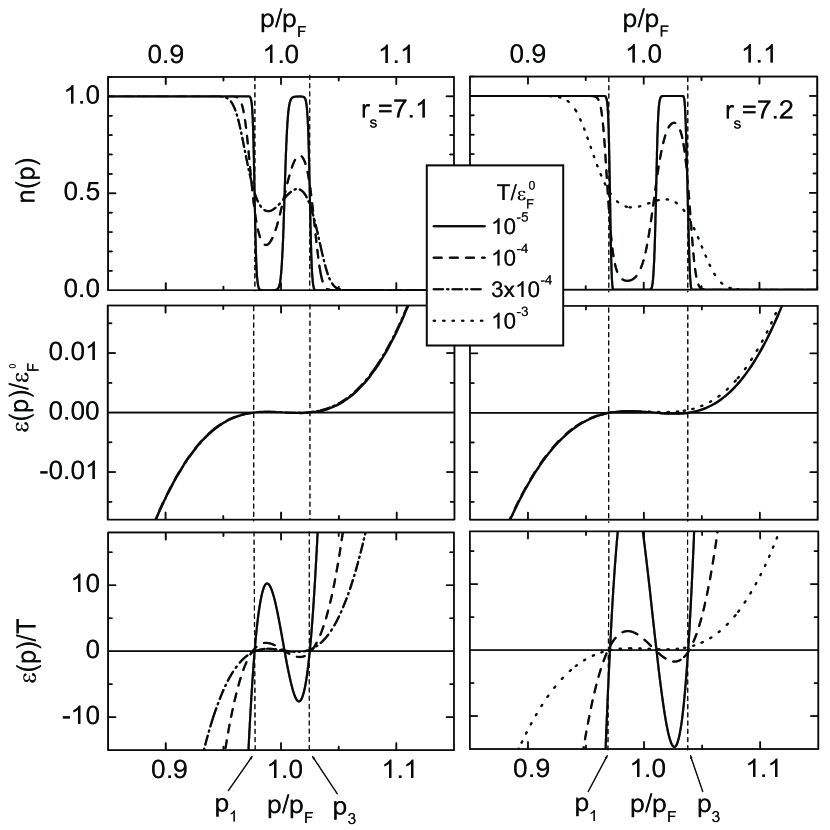
Figure 7: Occupation number $n(p)$ (top panels), single-particle spectrum $\epsilon(p)$ in units of $\epsilon_{F}^{0}$ (middle panels), and ratio $\epsilon(p)/T$ (bottom panels) for the interaction model (55) at $r_{s}=7.1$ (left column) and $r_{s}=7.2$ (right column), both exceeding the QCP value $r_{\infty}=7.0$. Interaction parameters are the same as for Fig. 6. All three quantities are plotted as functions of $p/p_{F}$ at different temperatures (measured in units $\varepsilon_{F}^{0}$) below the crossover temperature $T_{m}=10^{-3}\varepsilon^{0}_{F}$.

the alteration of the FL behavior in this temperature region is associated with crossover, rather than with some second-order phase transition. Nevertheless, comparison of Fig. 7 ($T<T_{m}$) and Fig. 8 ($T>T_{m}$) reveals striking changes in the structure of both of the functions $\epsilon(p)$ and $n(p)$. Indeed, as seen in the top panel of Fig. 7, a well-defined multi-connected Fermi surface, witnessed by a pronounced gap in filling, exists only at extremely low $T<10^{-4}\varepsilon^{0}_{F}$, while at $T\simeq T_{m}\simeq 10^{-3}\varepsilon^{0}_{F}$, the gap in the occupation numbers closes.

On the other hand, upon inspection of the top panel of Fig. 8, we observe that within a region region $p_{i}<p<p_{f}$ all of the curves for $n(p,T)$ for $T>T_{m}$ collapse into a single one—i.e., the momentum distribution $n(p)$ becomes $T$-independent. This behavior persists until rather high $T$. Fig. 8 also indicates that the range $\eta=p_{f}-p_{i}$ practically coincides with the difference-of-roots $\Delta p=p_{3}-p_{1}$ (cf. Subsec. III.A), so that in accordance with Eq. (28) we can write

$$\eta\sim\sqrt{\rho_{\infty}-\rho}\ .$$ (58)

Moreover, comparison of the bottom panels of Figs. 7 and 8 demonstrates that the huge variations of the ratio $\epsilon(p)/T$ that are so prominent at $T<T_{m}$ completely disappear in the FC domain at $T>T_{m}$. Thus, again we discover scaling behavior: within the range $p_{i}<p<p_{f}$ all of the curves representing the ratio $\epsilon(p)/T$ collapse into a single one.

The same conclusions follow from parallel calculations carried out for the interaction (56). For this case, Figs. 9 and 10, dedicated respectively to $T<T_{m}$ and $T>T_{m}$, trace the behavior with temperature of the spectrum $\epsilon(p)$ and momentum distribution $n(p)$.

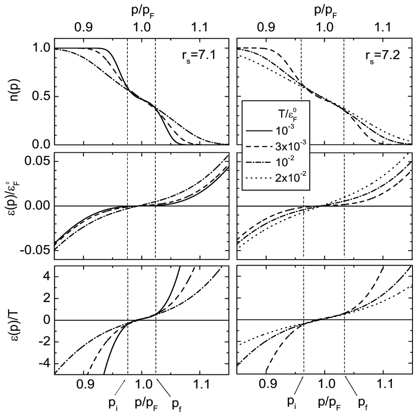
Figure 8: Same as in Fig. 7 but at temperatures above $T_{m}$.

Figure 9: Occupation numbers $n(p)$ (top panel), single-particle spectrum $\epsilon(p)$ in units of $10^{-3}\,\varepsilon_{F}^{0}$ (middle panel), and ratio $\epsilon(p)/T$ (bottom panel), plotted versus $p/p_{F}$ at three line-type-coded temperatures in units of $\varepsilon_{F}^{0}$, taken below the transition temperature $T_{m}=3\times 10^{-3}\,\varepsilon^{0}_{F}$. Interaction model (56) is assumed with parameters $g_{3}=0.45$ and $\beta_{3}=0.07$.

The scaling behavior observed in Figs. 7–10 is also evident in Fig. 11, where corresponding results of calculations based on Eq. (5) and the interaction model (57) are displayed. The single noteworthy difference is that the linear-in-$T$ dispersion of the single-particle spectrum $\epsilon(p)$ characteristic of the FC domain is already in effect at $T\to 0$, i.e., $T_{m}=0$ in this case. The results of similar numerical calculations for the singular interaction function (30), to be published separately, support the same general conclusions, in particular with respect to scaling behavior. From the evidence gathered for different singular interaction functions, we infer that scaling features that govern the flattening of single-particle beyond the QCP and at $T>T_{m}$ are universal. The specifics of the interaction function affect only the value of the crossover temperature $T_{m}$.

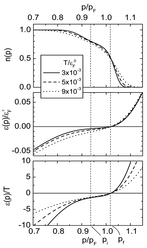
Figure 10: Same as in Fig. 9 but at temperatures above $T_{m}$.

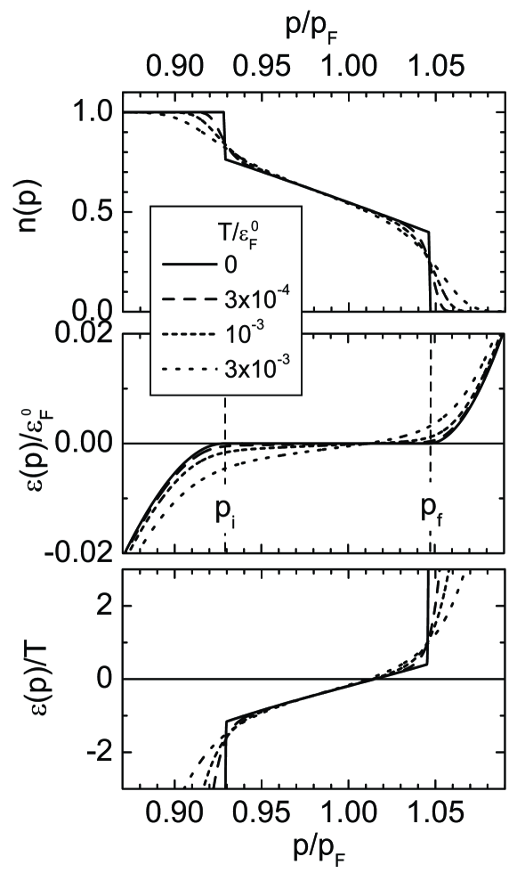
Figure 11: Occupation number $n(p)$ (top panels), single-particle spectrum $\epsilon(p)$ in units of $\varepsilon_{F}^{0}$ (middle panels), and ratio $\epsilon(p)/T$, (bottom panels) for the model (57) with the parameters $\beta=10$ and $g_{s}=70.0$. All three quantities are shown as functions of $p/p_{F}$ at different line-type-coded temperatures measured in units of $\varepsilon_{F}^{0}$.

VI Relevance of the QCP topological scenario to reality

Here we provide a brief assessment of the relevance of the theory outlined in this article to the contemporary experimental situation. At the outset we should emphasize that this theory is applicable only to systems whose properties are aptly described by the conventional FL approach on the weakly correlated side of the QCP. If this condition is not met, the theory is irrelevant.

At present, experimental information on the QCP is available for three types of strongly correlated Fermi systems. The first type is a silicon inversion layer in MOSFET, with the electrons forming a homogeneous 2D liquid. It is known from measurements of the magnetic susceptibility and the Shubnikov-de Haas oscillations sarachik ; pudalov ; shashrev ; dolgrev that the 2D electron gas does obey standard Landau theory on the FL side of the QCP. Furthermore, recent measurements shashprb carried out for two different versions of the crystal structure, namely $(100)$ and $(111)$, and for differing disorder have nevertheless demonstrated that the density at which the effective mass $M^{*}$ diverges remains the same, $\rho_{\infty}\simeq 0.8\times 10^{11}$ cm^-2. This finding implies that electron-electron interactions rather than disorder are responsible for the occurrence of the QCP in the silicon inversion layer. Moreover, the experimental value of the Stoner factor, which specifies the proximity to the ferromagnetic phase transition, is shown not to be enhanced relative to its value in the volume of the silicon crystal.shashrev This finding implies that ferromagnetism is irrelevant to the rearrangement of the ground state that takes place at the QCP. From the theoretical side, we have already mentioned that resultsbz from microscopic calculations bearing on the divergence of effective mass of the 2D electron gas are in agreement with the topological scenario for the QCP. All of the above factors, both empirical and computational, speak for the relevance of the proposed topological scenario to the reality of the 2D electron gas in the vicinity of the QCP.

Salient experimental information is also available for a second class of Fermi systems having a QCP: films of ³He atoms lying on different substrates. With certain qualifications, these systems may be modeled as 2D liquid ³He. If the dimensionless Landau parameters specifying the effective interaction between ³He atoms are rather small, the laboratory systems may found to obey standard FL theory. There is experimental evidence that this is indeed the casegodfrin ; saunders ; sscience —in spite of the violation of the Galilean invariance and the presence of disorder, effects introduced by the substrate. As reflections of a divergent density of states, the presence of the QCP in ³He films is exhibited in measurements of the spin susceptibility $\chi$,godfrin ; saunders and the specific heat $C$,saunders ; sscience with the quantitative results showing a substantial dependence on the nature of the substrate. A crucial feature of the measurementsgodfrin ; sscience is the curious Curie-like behaviorgodfrin ; sscience found for the spin susceptibility: $\chi(T,\rho)=C_{\mbox{\scriptsize eff}}(\rho)/T$, with the effective Curie constant $C_{\mbox{\scriptsize eff}}$ depending strongly on the density $\rho$ in the QCP region. The challenge of explaining this experimentally documented crossover from Pauli-like to Curie-like behavior is still open. A microscopic understanding is necessarily complicated by interactions between substrate and helium atoms and by layering effects at higher areal densities. In the next section we will see that the topological scenario for the QCP shows promise of capturing the essential physics of the crossover.

The third and most extensive class of systems possessing a QCP is that of the heavy-fermion metals, in which the crystal lattice gives rise to anisotropy of the Fermi surface. We have argued in Subsec. II.B.2 that short-range antiferromagnetic fluctuations cannot be relevant to the QCP in these systems. On the other hand, the existence of topological phase transitions in this class of systems is well known,lifshitz ; abr as pointed out in the same subsection. A priori there appear to be no serious obstacles to implementation of the topological QCP scenario for the heavy-fermion metals.

VII Unconventional thermodynamics beyond the QCP

Theoretical results based on the ideas and method we have developed allow one to reproduce available experimental data on properties of several concrete strongly-correlated Fermi systems in the immediate vicinity of the QCP (for example, see Refs. ckz, ; yak, ; kz2007, ). However, such validation is to some extent inconclusive, since as a rule there exist at least two alternative models that are capable of explaining the data at the same level of accuracy. Accordingly, in this section we will focus on certain unusual features of the thermodynamic properties of strongly correlated systems beyond the QCP that emerge in the proposed topological scenario. Detailed comparisons of the theory with experimental data is reserved for a future article.

VII.1 Entropy excess

In standard FL theory where the entropy $S$ is given by Eq. (3), the curve $S(T)$ starts at the origin and begins to rise linearly with $T$. The situation changes at the QCP. In the conventional scenario, which is predicated on a vanishing quasiparticle $z$-factor, one has $S(T)\sim C(T)\sim T\ln(1/T)$. In the topological scenario for the QCP, the divergence of the ratio $C(T)/T$ is even stronger:ckz $C(T)/T\sim T^{-2/3}$. The standard FL behavior of $C(T)/T$ does re-emerge beyond the QCP, where the density of states is again finite. However, recovery of this behavior occurs only at extremely low temperatures, with the proviso that $T<T_{m}$. At higher $T$, the FC forms in the domain $\Omega$, and its characteristic NFL momentum distribution, given by $n_{*}(p)$, leads to a drastic change in the behavior of the entropy $S(T)$.ks ; physrep ; zk4 ; yak The basic entropy formula (3) of the original quasiparticle formalism remains intact, but due to the NFL component in $n_{*}(p)$, the system is seen to possess a $T$-independent entropy excess $S_{*}(\rho)$. Its value does not depend of the manner of its evaluation, since Eq. (43) and (3) provide the same result.

The situation we now face—with the strongly correlated fermion system having a finite value $S_{*}$ of the entropy at $T=0$—resembles that encountered in a system of localized spins. In the spin system, the entropy referred to one spin is simply $\ln 2$, while in the system having a FC, we have $S_{*}/N\simeq\eta\ln 2$, where $\eta=\rho_{f}/\rho$ is the dimensionless FC parameter.

Numerical calculations demonstrate that within the domain $\Omega$, the momentum distribution $n_{*}(p)$ changes rapidly under variation of the total density $\rho$. The corresponding nonzero value of the derivative $\partial S_{*}/\partial\rho$ produces a huge enhancement of the thermal expansion coefficient $\beta\sim\partial S(T)/\partial\rho\simeq\eta$ with respect to its FL value, proportional to $T$.zksb Consonant with this result, experimental dataoeschler show that at low $T$ in many heavy-fermion metals, $\beta$ is indeed almost temperature-independent and exceeds typical values for ordinary metals by a factor $10^{3}$–$10^{4}$. To our knowledge, no theory has previously been advanced to explain this enhancement.

VII.2 Curie-Weiss behavior of the spin susceptibility

Another peculiar feature of strongly correlated Fermi systems beyond the QCP involves the temperature dependence of the spin susceptibility $\chi(T)=\chi_{0}(T)/(1+g_{0}\Pi_{0}(T))$, where

$$\chi_{0}=\mu^{2}_{e}\Pi_{0}(T)=-2\mu^{2}_{e}\int{dn(p,T)\over d\epsilon(p)}d\upsilon\,,$$ (59)

and $g_{0}$ is the spin-spin component of the interaction function (which remains unchanged through the critical density region). As mentioned before, beyond the QCP the standard Pauli behavior of $\chi(T)$ prevails only at $T<T_{m}$, and its value, proportional to the zero-temperature density of states $N(0)\sim|\rho-\rho_{\infty}|^{-1}$, turns out to be greatly enhanced.

At $T>T_{m}$, insertion of $n_{*}(p)$ into Eq. (59) yields the Curie-like term

$$\chi_{*}(T)=\mu^{2}_{e}{C_{\mbox{\scriptsize eff}}(\rho)\over T}\,,$$ (60)

with an effective Curie constant

$$C_{\mbox{\scriptsize eff}}(\rho)=2\int n_{*}(p)(1-n_{*}(p))d\upsilon$$ (61)

that depends dramatically on the density.zk4 ; yak Since $C_{\mbox{\scriptsize eff}}$ is proportional to the FC parameter $\eta$, we infer that

$$C_{\mbox{\scriptsize eff}}\simeq S_{*}\ .$$ (62)

Thus, all compounds in which the spin susceptibility exhibits the Curie-like behavior possess a large entropy. Furthermore, in the whole temperature interval from $T=0$ to $T>T_{m}$, the spin susceptibility of a Fermi system beyond the QCP possesses Curie-Weiss-like behavior $\chi(T)\sim 1/(T-T_{W})$ with a negative Weiss temperature $T_{W}$. Measurements in ³He films on various substratesgodfrin ; sscience and in numerous heavy-fermion compounds (cf. Refs. steglich3, ; tayama, ) provide examples of this NFL behavior. We emphasize that in our scenario, the negative sign of $T_{W}$ holds independently of the character of the spin-spin interaction, repulsive or attractive. (In the latter case, the magnitude of this interaction must not exceed certain limits, as indicated below in Subsec. VIII.B.) At the same time, in a system of localized spins the Weiss temperature has a negative sign only if the spin-spin interaction is repulsive. In this case, however, the Stoner factor must be suppressed. The necessity of reconciling the negative sign of $T_{W}$ with the enhanced Stoner factor observed experimentally in the vicinity of the QCPsteglich ; gegenwart creates insurmountable difficulties for the standard collective QCP scenario.

Another conspicuous feature of the physics beyond the QCP is associated with the Sommerfeld-Wilson ratio $R_{SW}=T\chi(T)/\mu^{2}_{e}C(T)\sim S_{*}/C(T)$. Since the excess entropy $S_{*}$ does not depend on $T$, it makes no contribution to the specific heat $C(T)$; consequently one should see a great enhancement of $R_{SW}$.

VIII Release of entropy stored in the fermion condensate

The diversity of phase transitions occurring at low temperatures is one of the most spectacular features of the physics of many heavy-fermion compounds. Within the standard collective scenario,hertz ; millis it is hard to understand why these transitions are so different from one another and their critical temperatures are so extremely small. However, such diversity is endemic to systems with a FC. Its source may be traced to an obvious fact: The existence of the excess entropy $S_{*}$ at $T=0$ would contradict the third law of thermodynamics (the Nernst theorem). We may recall that in order to relieve themselves of excess of the entropy, systems of localized spins order magnetically due to spin-spin interactions. The situation in systems with a FC is similar, but there are many ways to release the excess entropy $S_{*}$ as $T$ goes down to zero. One possible route for eliminating $S_{*}$, already considered, is the crossover between the state with a FC and a state with a multi-connected Fermi surface as the temperature drops below $T_{m}$. However, this is by no means a unique prescription for removing the entropy excess. Other options are associated with second-order phase transitions, involving violation of a symmetry of the ground state.

VIII.1 Superconducting phase transitions.

It is instructive to begin with superconducting phase transitions, considered already in the first articleks devoted to fermion condensation. A necessary condition for a superconducting transition to come into play is that its critical temperature $T_{c}$ exceeds $T_{m}$. To determine $T_{c}$, one sets $\Delta_{L}\to 0$ in the well-known BCS gap equation, yielding

$$\Delta_{L}(p,T\to 0)=\int{\cal V}_{L}(p,p_{1}){\tanh[\epsilon(p_{1})/2T]\over 2\epsilon(p_{1})}\Delta_{L}(p_{1},T)d\upsilon_{1}\,,$$ (63)

where ${\cal V}_{L}$ is the effective interaction between quasiparticles in the $L$-wave pairing channel. It can be demonstrated that the FC contribution to the integrand on the right-hand side of this equation is dominant. After some algebra employing the identity

$${{\tanh\left(\epsilon(p)/2T\right)}\over{\epsilon(p)}}={1-2n_{*}(p)\over T\ln\left[(1-n_{*}(p))/n_{*}(p)\right]}\ ,\quad{\bf p}\in\Omega\ ,$$ (64)

one obtains

$$T_{c}={\cal V}_{L}(p_{F},p_{F})\int_{\Omega}{1-2n_{*}(p)\over 2\ln\left[(1-n_{*}(p))/n_{*}(p)\right]}d\upsilon\ .$$ (65)

Confining the integration to the small FC domain, one arrive atks

$$T_{c}\simeq\lambda\eta\varepsilon^{0}_{F}\,,$$ (66)

where $\lambda$ is a dimensionless pairing constant and $\eta\sim|\rho-\rho_{\infty}|^{1/2}$ is the FC parameter. We see now that a remarkable situation arises if the pairing constant is large enough to ensure satisfaction of $T_{c}>T_{m}$. In contrast to the exponentially small BCS critical temperature $T_{c}\sim e^{-2/\lambda}$, the critical temperature in a system having a FC turns out to be a linear function of $\lambda$.

VIII.2 Phase transitions in the particle-hole channel

Along the same lines, we can consider the possibility of a collapse of particle-hole collective modes in systems with a FC. Here we restrict ourselves to long-wave transitions that give rise to a deformation of the Fermi surface. Manipulations similar those previously applied lead to the relation

$$O_{L}(p)=-\int{\cal F}_{L}(p,p_{1}){dn(p_{1})\over d\epsilon(p_{1})}O_{L}(p_{1})d\upsilon_{1}\ ,$$ (67)

where $O_{L}(p)$ is shape function characterizing the deformation. In the FC region we have $dn(p)/d\epsilon(p)=n_{*}(p)(1-n_{*}(p))/T$, so that upon retaining only the FC contribution Eq. (67) is recast as an equation for the transition temperature,

$$T_{N}=-{\cal F}_{L}(p_{F},p_{F})\int_{\Omega}n_{*}(p)(1-n_{*}(p))d\upsilon\simeq-f_{L}\eta\varepsilon^{0}_{F}\ .$$ (68)

On observing that the dimensionless Landau parameters $F_{L}=f_{L}/N(0)$ keep their values through the critical region, we may express the transition temperature in the form $T_{N}=F_{L}\eta/N(0)$. Remembering that the FC density $\eta$ is proportional to $|\rho-\rho_{\infty}|^{1/2}$, while the density of states behaves as $N(0)\sim|\rho-\rho_{\infty}|^{-1}$, the estimated value of $T_{N}$ appears to be proportional to $|\rho-\rho_{\infty}|^{3/2}$, being comparable with the crossover temperature $T_{m}$. In the case of ferromagnetism, the condition $T_{N}>T_{m}$ is met only if the spin-spin component of the interaction function is negative and sufficiently large. Otherwise, the system avoids the ferromagnetic phase transition and the spin susceptibility obeys the Curie-Weiss law $\chi(T)\sim 1/(T-T_{W})$ with a negative Weiss temperature $T_{W}$.

Remarkably, in either of the above candidates posed as a mechanism for release of the excess entropy $S_{*}$ through a symmetry-breaking second-order phase transition, the unconventional state with a FC always corresponds to the high-temperature phase, while the low-temperature phase possesses more familiar properties. Phase transitions occur in any channel where the sign of the effective interaction is suitable for the transition, provided the value of the effective coupling constant is sufficient to produce the inequality $T_{c}>T_{m}$. Otherwise, the entropy excess is released through the crossover leading to formation of a multi-connected Fermi surface. We see, then, that the diversity of phase transitions in the topological scenario for the QCP is due to the accumulation by the FC of a big entropy at extremely low temperatures. Because of the smallness of the parameter $|\rho-\rho_{\infty}|$, the transition temperatures appear to be very low and the phase transitions themselves inevitably of quantum origin. Several phases specified by different order parameters can in principle coexist with each other, giving rise to states of an intricate nature. As the temperature decreases to zero, these phases can replace one another.

IX Conclusion

A basic postulate of standard Fermi liquid theory reads: “At the transition from a Fermi gas to a Fermi liquid, the classification of energy levels remains unchanged” (Ref. lanl, , p. 11). Some 20 years ago, the first paper on the theory of fermion condensationks demonstrated that this postulate is incorrect beyond a quantum critical point, while maintaining the essence of the quasiparticle picture. The paper triggered a wave of criticism and disbelief; the judgment, “This theory is an artifact of the Hartree-Fock method,” was typical. By now, debates on the subject have become pointless: numerical calculations based on Eq. (5), carried out during the last decade and discussed in the present work, provide the best way to answer critics.

It has been a principal goal of this article to investigate the structure of the Fermi surface beyond the quantum critical point within the original Landau quasiparticle pattern.lan We have shown that at $T=0$ there are two different realizations of this pattern, both of which involve a topological phase transition. The first is associated with the emergence of a multi-connected Fermi surface. The second entails the formation of a fermion condensate, implicated by the emergence of completely flat portion of the single-particle spectrum $\epsilon(p)$ that may be envisioned as a virtual swelling of the Fermi surface. Such an inflation of the Fermi surface can occur if the Landau interaction function $f$ contains components of long range in coordinate space.

We have performed a series of numerical calculations that serve to demonstrate the existence of a crossover between the two types of topological structure at extremely low temperature, an effect that introduces a new energy scale $T_{m}$ into the problem. At $T>T_{m}$, both the momentum distribution $n(p)$ and the single-particle spectrum $\epsilon(p)$ exhibit universal features inherent in strongly correlated Fermi systems beyond the QCP. To be specific, scaling features pertaining to the behavior of the momentum distribution $n(p)$ and the (scaled) single-particle energy $\epsilon(p)/T$ in the vicinity of the Fermi surface are independent of the assumed form of the interaction function $f$ (and notably whether on not it contains long-range components). The choice of $f$ does, however, affect the value of $T_{m}$.

We have explored intriguing features of Poincaré mapping as a technique for iterative solution of the nonlinear integral equation (5) that connects the group velocity and the quasiparticle momentum distribution at zero temperature. For regular interaction functions, the sequence of iterative maps converges to the true solution beyond the quantum critical point and describe a new ground state with a multi-connected Fermi surface. However, if the Landau interaction function $f$ has a component of long range in coordinate space, 2-cycles are generated in the standard iteration procedure, a behavior symptomatic of the inadequacy of this solution algorithm as well as the failure of standard Fermi liquid theory beyond the quantum critical point. Adopting a refined iteration procedure (in which the input for the next step is a mixture of the outputs of the two preceding iterations), the spurious 2-cycles no longer arise. However, the new sequence of iterative maps acquires chaotic features in a region of momentum space adjacent to the Fermi surface that coincides with the domain in which the 2-cycles were previously found.

We have elaborated a special procedure for averaging the successive outputs of the iteration process and demonstrated that the averaged single-particle energies and occupation numbers so obtained coincide with those inherent in states with a fermion condensate. The exceptional states involving a fermion condensate are shown to possess a nonzero entropy at zero temperature. This result does not contradict basic laws of statistical physics if and only if the ground state is degenerate. In effect, the comprehensive analysis of Eq. (5) presented here affirms the consistency of the properties of states possessing a fermion condensate. The new insight into the role of chaos theory in the quantum many-body problem that has been gained through our analysis lays a basis for future studies with the potential of wide implications.

Finally, we have investigated pathways for releasing the entropy excess stored in the fermion condensate that are associated with different quantum phase transitions—necessarily of quantum origin since the transitions involved occur at extremely low temperatures.

References

- (1) L. D. Landau, Zh. Eksp. Teor. Fiz. 30, 1058, (1956) [Sov. Phys. JETP, 3, 920, (1957)].
- (2) C. Bäuerle, Yu. M. Bun’kov, A. S. Chen, S. N. Fisher, and H. Godfrin, J. Low Temp. 110, 333 (1998).
- (3) A. Casey, H. Patel, J. Nyeki, B. P. Cowan, and J. Saunders, Phys. Rev. Lett. 90, 115301 (2003).
- (4) M. Neumann, J. Nyeki, B. P. Cowan, and J. Saunders, Science 317, 1356 (2007).
- (5) O. Prus, Y. Yaish, M. Reznikov, U. Sivan, and V. Pudalov, Phys. Rev. B 67, 205407 (2003).
- (6) G. R. Stewart, Rev. Mod. Phys. 73, 797 (2001); 78, 743 (2006).
- (7) D. Takahashi, S. Abe, H. Mizuno, D. A. Tayurskii, K. Matsumoto, H. Suzuki, and Y. Onuki, Phys. Rev. B 67, 180407(R) (2003).
- (8) R. Kuc̈hler, N. Oeschler, P. Gegenwart, T. Cichorek, K. Neumaier, O. Tegus, C. Geibel, J. A. Mydosh, F. Steglich, L. Zhu, and Q. Si, Phys. Rev. Lett. 91, 066405 (2003).
- (9) P. Gegenwart, J. Custers, T. Tayama, K. Tenya, C. Geibel, O. Trovarelli, F. Steglich, and K. Neumaier, Acta Phys. Pol. B 34, 323 (2003).
- (10) J. Custers, P. Gegenwart, H. Wilhelm, K. Neumaier, Y. Tokiwa, O. Trovarelli, F. Steglich, C. Pepin, and P. Coleman, Nature 424, 524 (2003).
- (11) P. Gegenwart, J. Custers, Y. Tokiwa, C. Geibel, and F. Steglich, Phys. Rev. Lett. 94, 076402 (2005).
- (12) S. L. Bud’ko, E. Morosan, and P. C. Canfield, Phys. Rev. B 69, 014415 (2004); B 71, 054408 (2005).
- (13) H. Q. Yuan, M. Nicklas, Z. Hossain, C. Geibel and F. Steglich, Phys. Rev. B 74, 212403 (2006).
- (14) H. Q. Yuan, F. M. Grosche, M. Deppe, G. Sparn, C. Geibel and F. Steglich, Phys. Rev. Lett. 96, 047008 (2006).
- (15) J. Paglione, M. A. Tanatar, D. G. Hawthorn, F. Ronning, R. W. Hill, M. Sutherland, Louis Taillefer, and C. Petrovic, Phys. Rev. Lett. 97, 106606 (2006).
- (16) J. A. Hertz, Phys. Rev. B 14, 1165 (1976).
- (17) A. J. Millis, Phys. Rev. B 48, 7183 (1993).
- (18) P. Coleman, C. Pepin, Q. Si, and R. Ramazashvili, J. Phys.: Condens. Matter 13, R723 (2001).
- (19) B. Doniach and S. Engelsberg, Phys. Rev. Lett. 17, 750 (1966).
- (20) A. M. Dyugaev, Sov. Phys. JETP 43, 1247 (1976).
- (21) P. Gegenwart, Qimiao Si, and F. Steglich, cond-mat/07122045.
- (22) V. A. Khodel, cond-mat/07093653; JETP Lett. 86, 721 (2007).
- (23) L. D. Landau and E. M. Lifshitz, Statistical Physics, Vol. 2 (Pergamon Press, Oxford, 1980).
- (24) A. A. Abrikosov, L. P. Gor’kov, and I. E. Dzyaloshinski, Methods of Quantum Field Theory in Statistical Physics, (Prentice-Hall, London) 1963.
- (25) V. A. Khodel and V. R. Shaginyan, JETP Lett. 55, 110(1992).
- (26) M. V. Zverev, V. A. Khodel, and V. R. Shaginyan, JETP 82, 567 (1996).
- (27) A. V. Chubukov, V. M. Galitski, and V. M. Yakovenko, Phys. Rev. Lett. 94, 046404 (2005).
- (28) G. E. Volovik, Springer Lecture Notes in Physics 718, 31 (2007) [cond-mat/0601372].
- (29) V. V. Borisov and M. V. Zverev, JETP Letters 81, 503 (2005).
- (30) I. M. Lifshitz, JETP 11, 1130 (1960).
- (31) A. A. Abrikosov, J. C. Campuzano, and K. Gofron, Physica C214, 73 (1993).
- (32) L. D. Landau and E. M. Lifshitz, Hydrodynamics, (Fizmatlit 2003).
- (33) H. Frölich, Phys. Rev. 79, 845 (1950).
- (34) M. de Llano and J. P. Vary, Phys. Rev. C 19, 1083 (1979); M. de Llano, A. Plastino and J. G. Zabolitzky, Phys. Rev. C 20, 2418 (1979); V. C. Aguilera-Navarro, R. Belehrad, M. de Llano, M. Sandel, and J. P. Vary, O. Rojo, Phys. Rev. C 22, 1260 (1980); M. de Llano, A. Plastino, and J. G. Zabolitzky, Phys. Rev. C 22, 314 (1980).
- (35) C. J. Pethick, G. Baym, and H. Monien, Nucl. Phys. A 498, 313 (1989).
- (36) J. Quintanilla, A. J. Schofield, Phys. Rev. B 74, 115126 (2006).
- (37) M. V. Zverev and M. Baldo, JETP 87, 1129 (1998); J. Phys.: Condens. Matter 11, 2059 (1999).
- (38) S. A. Artamonov, V. R. Shaginyan, and Yu. G. Pogorelov, JETP Lett. 68, 942 (1998).
- (39) M. Feigenbaum, J. Stat. Phys. 21 69, (1979).
- (40) J. W. Clark, V. A. Khodel, and M. V. Zverev, Phys. Rev. B 71, 012401 (2005).
- (41) P. Nozières, J. Phys. I France 2, 443 (1992).
- (42) V. A. Khodel, J. W. Clark, Haochen Li, and M. V. Zverev, Phys. Rev. Lett. 98, 216404 (2007).
- (43) A. B. Migdal, Theory of Finite Fermi Systems and Applications to Atomic Nuclei (Wiley, New York, 1967).
- (44) P. Ring and P. Schuck, The Nuclear Many-Body Problem (Springer-Verlag, Berlin, 1980).
- (45) V. A. Khodel and V. R. Shaginyan, JETP Lett. 51, 553 (1990).
- (46) G. E. Volovik, JETP Lett. 53, 222 (1991).
- (47) D. V. Khveshchenko, R. Hlubina, and T. M. Rice, Phys. Rev. B 48, 10766 (1993).
- (48) V. A. Khodel, V. V. Khodel, and V. R. Shaginyan, Phys. Rep. 249, 1 (1994).
- (49) J. Dukelsky, V. A. Khodel, P. Schuck, and V. R. Shaginyan, Z. Phys. B102, (1997).
- (50) M. R. Norman, in High Temperature Superconductivity, edited by S. E. Barnes, J. Ashkenazi, J. L. Cohn, and F. Zuo (AIP, Woodbury, 1999), p. 298.
- (51) V. A. Khodel, M. V. Zverev, Physica B 312-313, 506 (2002).
- (52) V. Yu. Irkhin, A. A. Katanin, and M. I. Katsnelson, Phys. Rev. Lett. 89, 076401 (2002).
- (53) V. A. Khodel, M. V. Zverev, and J. W. Clark, JETP Lett. 81, 315 (2005).
- (54) V. A. Khodel, M. V. Zverev, and V. M. Yakovenko, Phys. Rev. Lett. 95, 236402 (2005).
- (55) V. R. Shaginyan, M. Ya. Amusia, and K. G. Popov, Phys. Uspekhi 50, 563 (2007).
- (56) S. V. Kravchenko and M. P. Sarachik, Rep. Prog. Phys. 67 1 (2004).
- (57) V. M. Pudalov, M. E. Gershenson, and H. Kojima, in Fundamental Problems of Mesoscopic Physics, NATO science series, edited by I. V. Lerner, B. L. Altshuler, and Y. Gefen, p. 309 (Kluwer Academic Publ., Dordrecht, 2004).
- (58) A. A. Shashkin, Phys. Uspekhi 48, 129 (2005).
- (59) V. T. Dolgopolov, Low Temp. Phys. 33, 98 (2007).
- (60) A. A. Shashkin, A. A. Kapustin, E. V. Deviatov, V. T. Dolgopolov, and Z. D. Kvon, Phys. Rev. B 76, 241302(R) (2007).
- (61) M. V. Zverev, V. A. Khodel, V. R. Shaginyan, and M. Baldo, JETP Lett. 65 (1997) 863.
- (62) N. Oeschler, P. Gegenwart, M. Lang, R. Movshovich, J. L. Sarrao, J. D. Thompson, and F. Steglich, Phys. Rev. Lett. 91, 076402 (2003).
- (63) M. V. Zverev and V. A. Khodel, JETP Lett. 79, 635 (2004).
- (64) T. Tayama, A. Harita, T. Sakakibara, Y. Haga, H. Shishido, R. Settai, and Y. Onuki, Phys. Rev. B 65, 180504(R)(2002).
- (65) V. A. Khodel and M. V. Zverev, JETP Lett. 85, 404 (2007).