A unified approach to split absorbing boundary conditions
for nonlinear Schrödinger equations

Abstract

An efficient method is proposed for numerical solutions of nonlinear Schrödinger equations in an unbounded domain. Through approximating the kinetic energy term by a one-way equation and uniting it with the potential energy equation, absorbing boundary conditions are designed to truncate the unbounded domain, which are in nonlinear form and can perfectly absorb the waves outgoing from the truncated domain. We examine the stability of the induced initial boundary value problems defined on the computational domain with the boundary conditions by a normal mode analysis. Numerical examples are given to illustrate the stable and tractable advantages of the method.

I Introduction

In this paper, we consider the construction of absorbing boundary conditions (ABCs) for the nonlinear Schrödinger equation (NLS),

$$i\hbar\frac{\partial\psi(x,t)}{\partial t}=\left[-\frac{\hbar^{2}}{2m}\frac{\partial^{2}}{\partial x^{2}}+V(x)+f(|\psi|^{2})\right]\psi,$$ (1)

where $m$ is the atomic mass, $\hbar$ represents the Planck constant, and $V(x)$ is the potential function. This equation appears in many different applications SS:Book:99 ; Agr:BOOK:01 ; PS:Book:03 , such as the gravity waves on deep water in fluid dynamics, the pulse propagations in optics fibers, and the Bose-Einstein condensation. For the cubic nonlinear term $f(|\psi|^{2})\psi=g|\psi|^{2}\psi$, Eq. (1) reduced to Gross-Pitaevskii equation, which be numerically studied by phe1 ; phe2 ; bao and references therein. For a quintic nonlinearity, one can see phe3 .

A current challenge for the numerical solutions of this kind of problems is due to the unboundedness of the physical domain. The common practice to overcome this difficulty is to limit the computational domain and solve a reduced problem. To make the truncated problems complete, boundary conditions should be added to the reduced problem. ABCs applied at prescribed artificial boundaries have been widely studied in recent decades, such as Enguist:Majda:1977 ; Higdon:1986 for hyperbolic wave equations, Han:Wu:1985 ; Yu:1985 for elliptic equations, Halpern:Rauch:1995 ; Han:Huang:2002 for parabolic equations; see also the reviews by GivoliGivali:Elsevier , TsynkovS:ANM , HagstromTH:AN:1999 and HanHan:2006 . The purpose of designing ABCs is to annihilate all the incident waves so that minor reflected waves may propagate into the computational domain. ABCs can be distinguished into two categories: the global ABCs and local ABCs. The global ABCs usually lead to the well-approximated and well-posed truncated problems, but the implementation cost for the global ABCs is expensive. Fast evaluation methods Jiang:Greengard:CMA:2004 should be applied to treat the global ABCs. On the other hand, local ABCs are computationally efficient, but the accuracy and stability are the main concerns. There is another way to design ABCs based on the media of the material, called the perfectly matched layer (PML) methods berenger , which have been applied to many complicated wave propagation problems.

For the nonlinear equations, however, it is difficult to find a suitable boundary condition on the artificial boundary in general, except for some special cases such as the problem can be linearized Hagstrom:Keller:MC:1987 , or a Burgers type questions HXW:JCM:2006 ; WZ:CMA ; XHW:CICP:2006 which can be corresponded with the linear parabolic equations by the Cole-Hopf transformation. For the NLS equation on the unbounded domain, Zheng Zhe:JCP:06 obtained the transparent boundary condition using the inverse scattering transform approach for the cubic nonlinear Schrödinger equation in one dimension. Antonie et al. ABD:SINA:06 also studied the one-dimensional cubic nonlinear Schrödinger equation and constructed several nonlinear integro-differential artificial boundary conditions. In Sze:CMAME:06 ; Sze:NM:06 , Szeftel designed absorbing boundary conditions for one-dimensional nonlinear wave equation by the potential and the paralinear strategies. Soffer and StucchioSS:JCP:07 presented a phase space filter method to obtain absorbing boundary conditions. The PML FL:JOB:05 ; zheng was also applied to handling the nonlinear Schrödinger equations. The recent papers XH:PRE:06 ; XHW:arxiv:06 , split local absorbing boundary (SLAB) conditions have been developed through a time-splitting procedure for one-dimensional nonlinear Schrödinger equations. The local absorbing boundary conditions were imposed on the split linear subproblem and yielded a full scheme by coupling the discretizations for the interior equation and boundary subproblems. In addition, an adaptive method was developed to determine the parameter $k_{0}$ involved in the local boundary conditions.

In this paper, we present an efficient implementation of the nonlinear absorbing boundary conditions for the NLS equation by making use of the splitting idea XH:PRE:06 ; XHW:arxiv:06 . We distinguish incoming and outgoing waves along the boundaries for the linear kinetic subproblem, and then unite the potential energy subproblem to yield nonlinear boundary conditions which are of local form and examine the coupling between the equation governing the wave in the computational domain and the boundary conditions on the boundary yields a well-posed problem. Furthermore, the obtained boundary conditions are “easy” to discretize and “cheap” to compute in terms of the computational time. We will then perform numerical tests to illustrate the effectiveness and tractability of this approach.

II Nonlinear absorbing boundary conditions

II.1 Linear Schrödinger equation

Let us first consider the local ABCs of the linear Schrödinger equation,

$$i\hbar\frac{\partial\psi(x,t)}{\partial t}=-\frac{\hbar^{2}}{2m}\frac{\partial^{2}\psi}{\partial x^{2}},$$ (2)

which will be the basis of constructing ABCs of nonlinear problems, because it is the kinetic part of the NLS equation (1).

In the frequency domain of the Fourier transform, the one way equations at the two boundaries, which annihilate all the outgoing waves, can be represented by

$$i\sqrt{\frac{\hbar}{2m}}\hat{\psi}_{x}\pm\sqrt{\omega}\hat{\psi}=0,$$ (3)

where the subscript represents the partial derivative, $\hat{\psi}(x,\omega)$ is the Fourier transform of $\psi(x,t)$, $\omega$ is the frequency, the plus sign in “$\pm$” corresponds to the right boundary condition, and the minus sign corresponds to the left. The transparent boundary conditions in exact manner of the problem is then derived by an inverse Fourier transform:

$$i\sqrt{\frac{\hbar}{2m}}\psi_{x}\pm\frac{e^{-\frac{\pi}{4}i}}{\sqrt{\pi}}\frac{d}{dt}\int_{0}^{t}\psi(x,\tau)\frac{d\tau}{\sqrt{t-\tau}}=0,$$ (4)

which is a nonlocal boundary condition. In order to get local boundary conditions, a usual way is to approximate the square root $\sqrt{\omega}$ by using polynomials or rational polynomials. For instance, applying the approximations

$$\sqrt{\omega}=\sqrt{\omega_{0}}+O(\omega-\omega_{0}),$$ (5)

$$\sqrt{\omega}=\frac{\sqrt{\omega_{0}}}{2}+\frac{\omega}{2\sqrt{w_{0}}}+O(\omega-\omega_{0})^{2},$$ (6)

$$\sqrt{\omega}=\frac{\sqrt{\omega_{0}}(3\omega+\omega_{0})}{\omega+3\omega_{0}}+O(\omega-\omega_{0})^{3},$$ (7)

we obtain the first three absorbing boundary conditions in the physical domain:

$$\mathrm{1st~{}order}:~{}~{}~{} i\sqrt{\frac{\hbar}{2m}}\frac{\partial\psi}{\partial x}\pm k_{0}\psi=0,$$ (8)

$$\mathrm{2nd~{}order}:~{}~{}~{} i\psi_{t}\pm i\sqrt{\frac{2\hbar}{m}}k_{0}\frac{\partial\psi}{\partial x}+k_{0}^{2}\psi=0,$$

$$\mathrm{3rd~{}order}:~{}~{}~{} \frac{3i\hbar k_{0}^{2}}{m}\frac{\partial\psi}{\partial x}-2\frac{\partial^{2}\psi}{\partial x\partial t}\pm\left(\frac{\hbar k_{0}^{3}}{m}\psi+6ik_{0}\frac{\partial\psi}{\partial t}\right)=0.$$

Here, $\omega_{0}$ is a positive constant, and $k_{0}=\sqrt{\omega_{0}}$ which is called the wavenumber parameter.

II.2 Nonlinear absorbing boundary conditions

In this section, we derive the absorbing boundary conditions for the one-dimensional NLS equation (1) on the region $\Omega=[x_{l},x_{r}]$ by assuming that there do not exist outgoing waves at the two ends $x_{l}$ and $x_{r}$. We remark that this assumption is not correct for a general wave due to the nonlinear or space-dependent potential Zheng:CCP:08 , but it is reasonable for many situations of physical applications; in fact, this is a fundamental assumption so that we can design absorbing boundary conditions.

To understand the philosophy of obtaining nonlinear absorbing boundary conditions, let us rewrite Eq. (1) into the following operator form:

$$i\hbar\frac{\partial\psi(x,t)}{\partial t}=[\hat{T}+\hat{V}]\psi(x,t),$$ (9)

where $\hat{T}$ represents the linear differential operator which accounts for the kinetic energy part, and $\hat{V}$ is the nonlinear operator that governs the effects of the potential energy and nonlinearity. These are given by

$$\hat{T}=-\frac{\hbar^{2}}{2m}\frac{\partial^{2}}{\partial x^{2}},~{}~{}~{}\mathrm{and}~{}~{}~{}\hat{V}=V(x)+f(|\psi|^{2}).$$ (10)

In a time interval from $t$ to $t+\tau$ for small $\tau$, the exact solution of Eq. (9) can be approximated by

$$\psi(x,t+\tau)\approx e^{-i[\hat{T}+\hat{V}]\tau/\hbar}\psi(x,t)\approx e^{-i\hat{T}\tau/\hbar}e^{-i\hat{V}\tau/\hbar}\psi(x,t).$$ (11)

This means in a small time step $\tau$ that the approximation carries out the wave propagation in a kinetic energy step and a potential energy step separately. This is the basic idea of the well-known time-splitting method (or the split-step method) which is effective to numerically solve the nonlinear Schrödinger-type equations.

Since we have assumed that there are no outgoing waves on the artificial boundaries $x_{l}$ and $x_{r}$, noticing formulae (8), the kinetic operator $\hat{T}$ can be approached by one-way operators

$$\hat{T}\approx\hat{\mathcal{T}}^{(2)}=-\hbar\left(\pm i\sqrt{\frac{2\hbar}{m}}k_{0}\frac{\partial}{\partial x}+k^{2}_{0}\right),$$ (12)

$$\hat{T}\approx\hat{\mathcal{T}}^{(3)}=-\hbar^{2}\left(2i\frac{\partial}{\partial x}\pm 6k_{0}\right)^{-1}\left(\frac{3ik_{0}^{2}}{m}\frac{\partial}{\partial x}\pm\frac{k_{0}^{3}}{m}\right),$$ (13)

which correspond to the second- and third- order local boundary conditions in Eq. (8), respectively. Here, we also take the positive sign in “$\pm$” at $x=x_{r}$ and take the negative sign at $x_{l}$. Substituting $\hat{\mathcal{T}}^{(n)}$ for $\hat{T}$ in Eq. (11) yields approximating operators to the solution operator as follows,

$$e^{-i[\hat{T}+\hat{V}]\tau/\hbar}\approx e^{-i[\hat{\mathcal{T}}^{(n)}+\hat{V}]\tau/\hbar},$$ (14)

which imply the one-way equations,

$$i\hbar\frac{\partial\psi(x,t)}{\partial t}=[\hat{\mathcal{T}}^{(n)}+\hat{V}]\psi(x,t).$$ (15)

They approximate to Eq. (9) at two boundaries and being going to act as absorbing boundary conditions we need. Concretely, we obtain nonlinear absorbing boundary conditions:

$$n=2:~{}~{}~{} i\hbar\frac{\partial\psi}{\partial t}=\left[-\hbar(\pm i\sqrt{\frac{2\hbar}{m}}k_{0}\frac{\partial}{\partial x}+k_{0}^{2})+V(x)+f(|\psi|^{2})\right]\psi$$ (17)

$$n=3:~{}~{}~{} i\hbar\left(2i\frac{\partial}{\partial x}\pm 6k_{0}\right)\frac{\partial\psi}{\partial t}=\left[-\frac{\hbar^{2}}{m}\left(3ik_{0}^{2}\frac{\partial}{\partial x}\pm k_{0}^{3}\right)\right.$$

$$~{}~{}~{}~{}~{}~{}~{}~{}~{}~{}~{}~{}~{}~{}\left.+\{V(x)+f(|\psi|^{2})\}\left(2i\frac{\partial}{\partial x}\pm 6k_{0}\right)\right]\psi.$$

Here, in order to increase the accuracy of the boundary conditions, the wavenumber parameter $k_{0}$ is a function of time $t$, which will be determined by a windowed Fourier transform method XHW:arxiv:06 based on the frequency property of the wave function near the artificial boundaries. We express the boundary conditions (17) and (17) in the operator forms:

$$\mathbb{B}_{-}^{(n)}(x,t)\psi(x,t)=0,$$ (18)

$$\mathbb{B}_{+}^{(n)}(x,t)\psi(x,t)=0,$$ (19)

where $\mathbb{B}_{-}$ and $\mathbb{B}_{+}$ respectively represent the left and right boundary conditions; that is, the minus sign in $``\pm"$ is taken for $\mathbb{B}_{-}$, and the plus sign for $\mathbb{B}_{+}$. The initial value problem on the open domain of Eq. (1) restricted to the truncated interval $[x_{l},x_{r}]$ is then approximated by an initial boundary value problem with local absorbing boundary conditions:

$$i\hbar\frac{\partial\psi(x,t)}{\partial t}=\left[-\frac{\hbar^{2}}{2m}\frac{\partial^{2}}{\partial x^{2}}+V(x)+f(|\psi|^{2})\right]\psi,~{}~{}\mathrm{for}~{}~{}x\in[x_{l},x_{r}],$$ (20)

$$\psi(x,0)=\psi_{0}(x),~{}~{}\mathrm{for}~{}~{}x\in[x_{l},x_{r}],$$ (21)

$$\mathbb{B}_{-}^{(n)}(x_{l},t)\psi(x_{l},t)=0,~{}~{}\mathrm{for}~{}~{}n=2,~{}\mathrm{or}~{}3,$$ (22)

$$\mathbb{B}_{+}^{(n)}(x_{r},t)\psi(x_{r},t)=0,~{}~{}\mathrm{for}~{}~{}n=2,~{}\mathrm{or}~{}3.$$ (23)

II.3 Well-posedness of the induced IBVP

It is natural to examine the well-posedness that we concern most of the induced initial boundary value problem confined in the finite computational interval for the nonlinear Schrödiger equation by using the nonlocal absorbing boundary condition. The classical energy method seems to be difficult to obtain the stability result of the problem under consideration here. In this section, we will investigate the stability based on Kreiss’s normal mode analysis methodKL:book ; Fevens:Jiang:siam and references therein, which was also used for the wave equations and the linear Schrödinger equation.

The idea of the general algebraic normal mode analysis is based on the fact that the well-posed problem does not admit any complex eigenvalues with positive real parts $\hbox{Re}(s)>0$, or generalized eigenvalues with $\hbox{Re}(s)=0$ and the negative (positive) group velocity of normal mode on the right-hand (left-hand) boundary. The eigenvalues and generalized eigenvalues satisfy the dispersion relations of both the interior equation and the equation on the boundaries. If there exist such eigenvalues, the problem will admit an unboundedly grown normal mode $e^{st}$ and is hence unstable. If there exit such generalized eigenvalues, the boundary conditions will admit a incoming wave which will propagate energy into the interior domain to disrupt the solution in the computational interval and generate a spurious wave solution.

We need to check if there exist eigenvalues and generalized eigenvalues by replacing the solution of the plane wave form $\psi(x,t)=e^{st+kx}$ into Eq. (20) and boundary conditions (22)(23). There are left-hand and right-hand boundary, they can be considered by the same argument. Here we only consider the wellposedness with the right-hand boundary conditions. For n=2, substituting the plane wave into the dispersion relation and the boundary condition yields

$$i\hbar s=-\frac{\hbar^{2}}{2m}k^{2}+[V(x)+f(|\psi|^{2})],$$ (24)

$$i\hbar s=-i\hbar\sqrt{\frac{2\hbar}{m}}k_{0}k-\hbar k^{2}_{0}+[V(x)+f(|\psi|^{2})].$$ (25)

In very small time step $\tau$ the basic idea of the well-known time-splitting method is to carry out the wave propagation in a kinetic energy step and a potential energy step separately. When time step is taken limit to zero, that is the reason why we can write the nonlinear shrödinger equation in above forms, the nonlinear term is considered as a potential function. Hence, let (24) minus (25) and substitute the result into (24) to arrive at

$$k=i\sqrt{\frac{2m}{\hbar}}k_{0}~{}~{}\mathrm{and}~{}~{}s=-ik_{0}^{2}-i\frac{v_{1}+f_{1}}{\hbar}+\frac{v_{2}+f_{2}}{\hbar},$$ (26)

where $V+f=v_{1}+f_{1}+i(v_{2}+f_{2})$. For the $3\hbox{rd}$ order approximation on the right boundary, by the same argument, we have

$$i\hbar s=-\frac{\hbar^{2}}{2m}k^{2}+[V(x)+f(|\psi|^{2})],$$ (27)

$$i\hbar s=-\frac{\hbar^{2}k_{0}^{2}}{2m}\frac{3ik+k_{0}}{ik+3k_{0}}+[V(x)+f(|\psi|^{2})].$$ (28)

Combine (27) and (28), we have

$$\frac{\hbar^{2}}{2m}k^{2}-\frac{\hbar^{2}k_{0}^{2}}{2m}\frac{3ik+k_{0}}{ik+3k_{0}}=0,$$ (29)

solve (29) and substitute the results $k=ik_{0}$ into (27) to obtain

$$s=-i\frac{\hbar}{2m}k_{0}^{2}-\frac{i[V(x)+f(|\psi|^{2})]}{\hbar}$$ (30)

$$s=-i\frac{\hbar}{2m}k_{0}^{2}-i\frac{v_{1}+f_{1}}{\hbar}+\frac{v_{2}+f_{2}}{\hbar}.$$ (31)

It is easy to have $\mathrm{Re}(s)\leq 0$ for $v_{2}+f_{2}\leq 0$ from (26) and (31) whatever $n=2$ or $n=3$.

In particular, when $V$ and $f$ are both real functions, i.e. $v_{2}+f_{2}=0$, we thus have $\mathrm{Re}(s)=0,$ hence $s$ is wholly imaginary. Since the boundary condition is designed to annihilate all the outgoing wave, this implies that the group velocity is positive on the right-hand boundary. Hence there is no generalized eigenvalue which will propagate energy into the interior interval to influence on the true wave solution. If any instabilities which might be admitted by the generalized eigenvalues of the ABCs exit, they would not propagate wave to affect the interior solution. Keep this concept in mind, by linearizing the nonlinear terms in a sufficiently small time step, we can say that the boundary conditions of the problem (20)-(23) are well-posed if functions $V(\cdot)$ and $f(\cdot)$ satisfy $v_{2}+f_{2}\leq 0$. Hence the boundary condition for n=2 or 3 is well-posed and numerical tests below show that the boundary condition is stable.

III Numerical examples

In this section we will test the efficiency of the nonlinear absorbing boundary conditions by using the finite-difference scheme to the induced initial boundary value problem (20)-(23).
In the computational interval $[x_{l},x_{r}],$ let $J$ is a positive integer, denote $\Delta x=(x_{r}-x_{l})/J$ and $\Delta t$ by grid sizes in space and time, respectively. We use the following Crank-Nicolson-type difference scheme duan ; chang

$$i\hbar\frac{\psi^{n+1}_{j}-\psi_{j}^{n}}{\Delta t}=-\frac{\hbar^{2}}{2m}\frac{\psi^{n+\frac{1}{2}}_{j+1}-2\psi_{j}^{n+\frac{1}{2}}+\psi^{n+\frac{1}{2}}_{j-1}}{\Delta x^{2}}+[V_{j}+f(|\psi^{n+\frac{1}{2}}|^{2})]\psi_{j}^{n+\frac{1}{2}},$$

(32)

to discretize the nonlinear Schrödinger equation inside the computational domain, which is unconditionally stable and of second order in time. Here $\psi_{j}^{n+\frac{1}{2}}=\frac{\psi_{j}^{n+1}+\psi_{j}^{n}}{2}$ and $\psi_{j}^{n}$ represents the approximation of wave function $\psi$ at the grid point $(x_{j},t^{n})$ with $j=0,1,...,J,$ $x_{0}=x_{l},~{}x_{j}=x_{l}+j\Delta x,~{}x_{J}=x_{r},$ and $t^{n}=n\Delta t$. Obviously, the above systems of equations can not be solved uniquely since the number of equations are less than that of unknowns. At the two unknown ghost points $x_{-1}$ and $x_{J+1}$ no equation can be defined from (32). Thus the absorbing boundary conditions are required to provide two extra equations on the grid points $x_{s}$ for $s\in S=\{-1,0,1\}\cup\{J-1,J,J+1\}$ in the vicinity of boundary. The $3\hbox{rd}$ order ABCs are discretized as follows:

$$\left[\frac{3\hbar^{2}k_{0}^{2}i}{m}-2i(V_{s}+f(|\psi_{s}^{n+\frac{1}{2}}|^{2})\right]\frac{\psi_{s+1}^{n+\frac{1}{2}}-\psi_{s-1}^{n+\frac{1}{2}}}{2\Delta x}-\hbar\frac{\psi_{s+1}^{n+1}-\psi_{s-1}^{n+1}}{\Delta x\Delta t}+\hbar\frac{\psi_{s+1}^{n}-\psi_{s-1}^{n}}{\Delta x\Delta t}$$

$$\pm 6k_{0}i\frac{\psi_{s}^{n+1}-\psi_{s}^{n}}{\Delta t}\pm\left(\frac{\hbar^{2}k_{0}^{3}}{m}-6k_{0}V_{s}-6k_{0}f(|\psi_{s}^{n+\frac{1}{2}}|^{2})\right)\psi_{s}^{n+\frac{1}{2}}=0,$$ (33)

where the positive sign in $``\pm"$ corresponds to the right boundary $s=J$ and the negative one corresponds to the left boundary $s=0.$ The above scheme is implicit, we need use an iterative strategy to solve the nonlinear equations (32)-(33) by replacing $f(|\psi_{j}^{n+\frac{1}{2}}|^{2})$ with $f(|\frac{(\psi_{j}^{n+1})^{k}+\psi_{j}^{n}}{2}|^{2})$, where the superscript $k$ denotes the $k$-th iteration at each time step and the initial iteration is given as $(\psi_{j}^{n+1})^{0}=\psi_{j}^{n}$.
Without loss of generality, we rewrite the original NLS equation (1) as

$$i\psi_{t}=-\psi_{xx}+gf(|\psi|^{2})\psi+V\psi,$$ (34)

where $gf(|\psi|^{2})\psi$ represents different physical phenomena when chosen different nonlinear forms. In example 1, we take $f(|\psi|^{2})=|\psi|^{2}$, $V=0$ and $g=-2$, which corresponds to a focusing $(g<0)$ effect of the cubic nonlinearity. Many applications in science and technology have connections with this kind of NLS equations SS:Book:99 ; Agr:BOOK:01 ; PS:Book:03 . Furthermore, in this case equation (34) can be solved analytically by the inverse scattering theory, its exact soliton solution has the following form

$$\psi(x,t)=A\sqrt{\frac{-2}{g}}\hbox{sech}(Ax-2ABt)e^{iBx+i(A^{2}-B^{2})t},$$ (35)

where $A$ and $B$ are real parameters:$A$ determines the amplitude of the wavefield and $B$ is related to velocity of the soliton. In example 2, we take $f(|\psi|^{2})=|\psi|^{4}$, $V=0$ and $g=-2$, the NLS equation becomes of a quintic nonlinearity. The computational interval is set to be $[x_{l},x_{r}]=[-5,5].$ For this kind of NLS equation with power-like nonlinearity, if the initial energy satisfies:

$$E(\psi_{0}):=||\nabla\psi_{0}||_{L^{2}}^{2}-\frac{2}{3}||\psi_{0}||^{6}_{L^{6}}<0,$$ (36)

the solution $\psi$ will blow up in finite time (carles and references therein), i.e, there exists $T>0$ such that

$$\lim\limits_{t\rightarrow T}||\nabla_{x}\psi||_{L^{2}}\rightarrow+\infty.$$

In example 3, we take $f(|\psi|^{2})=|\psi|^{2}$, $V\neq 0$ and $g=2$, the NLS equation represents a nonlinear wave with repulsive interaction.
Example 1. We first consider the case of $g=-2$ and the temporal evolution of an initial bright solition

$$\psi(x,0)=\hbox{sech}(x-x_{0})e^{2i(x-x_{0})}$$ (37)

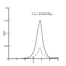
Figure 1: Evolution of the error $|\psi_{exa}-\psi_{h}|$ on the artificial boundary point .

with $x_{0}=15$. The exact solution is the form of (35) with $A=1$ and $B=2$. This case is used to test the performance of the nonlinear ABCs when the wave impinges on the right-hand-side boundary of the computational interval $[0,30]$. FIG. 1 shows the evolution of absolute error $|\psi_{exa}-\psi_{h}|$ on the artificial boundary point by picking wavenumber $k_{0}=2$, spatial size $\Delta x=0.1$ and time size $\Delta t=0.01$ and its refinement mesh. When refining the mesh, one can see that the error will converge quickly. In order to explore the convergence rates in space and time, we take time size as $\Delta t=\Delta x^{2}$. Denote the $L_{1}-$norm by

$$E_{1}=\frac{1}{(J+1)(N+1)}\sum\limits_{j=0}^{J}\sum\limits_{n=0}^{N}|\psi_{j}^{n}-\psi_{exa}(x_{j},t^{n})|.$$ (38)

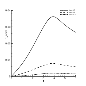
Figure 2: The evolution of the $L_{1}-$error versus time $t$ with refinement meshes.

FIG. 2 shows the evolution of the $L_{1}-$norm with different mesh sizes. From this figure, we observe a second-order accuracy of the errors. To character convergence rates exactly, we take the different values of the $L_{1}$-norm at different times and mesh sizes. TABLE I shows the second-order convergence rate.

Table 1: The values and orders of $L_{1}$-norm at different times and mesh sizes.

	$\Delta x=0.2$	order	$\Delta x=0.1$	order	$\Delta x=0.05$	order
$t=2$	1.570e-2	–	4.149e-3	2.076	1.017e-3	2.029
$t=3$	2.946e-2	–	6.797e-3	2.116	1.656e-3	2.037
$t=4$	3.622e-2	–	8.091e-3	2.162	1.955e-3	2.049
$t=5$	3.145e-2	–	6.948e-3	2.178	1.724e-3	2.011
$t=6$	2.691e-2	–	6.010e-3	2.163	1.581e-3	1.926

Another important method Fevens:Jiang:siam to see the influence of $k_{0}$ on the boundary conditions is the reflection ratios. The reflection ratios kuska:PRB are calculated as follow

$$r=\sum\limits_{j=0}^{J}|\psi_{j}^{n}|\left/\sum\limits_{j=0}^{J}|\psi_{j}^{0}|\right.,$$ (39)

which is efficient to measure the performance of nonlinear ABCs. $r=0$ implies that the soliton passes through the boundary completely, and $r=1$ indicates that the wave is completely reflected into the computational domain. In the experiments of BECs, g often takes larger value so that the nonlinear term will become very strong. TABLE II presents the reflection ratios with parameters g being chosen -2 and -10, respectively. We observed the wave numbers $k_{0}$ influence the reflection ratios under spatial size $\Delta x=0.1$ and time size $\Delta t=0.05$. But the reflection rates $r$ are insensitive to $k_{0}$, which can be taken in a large interval $[1.0,5.0]$ such that the reflection ratios is less than $1\%$. Out of the interval $r$ will increase rapidly. Furthermore, whatever the parameter g is given large or small, i.e. whatever the nonlinear term is strong or not, the reflection ratios are insensitive to the nonlinear term, either. The parameter g can even be chosen in a larger interval. FIG. 3 plots the amplitude of the soliton under $k_{0}=2.0$ and spatial size $\Delta x=0.1$, respectively. No reservable reflections can be detected at all.

Table 2: The values and orders of $L_{1}$-norm at different times and mesh sizes.

$g\setminus k_{0}$	0.5	0.75	1.0	1.25	1.5	1.75	2.0	2.125	2.25
$-2$	6.07e-2	1.601e-2	4.70e-3	1.52e-3	5.17e-4	1.81e-4	7.30e-5	6.13e-5	7.06e-5
$-10$	6.07e-2	1.60e-2	4.70e-3	1.52e-3	5.17e-4	1.81e-4	7.30e-5	6.13e-5	7.05e-5
$g\setminus k_{0}$	2.5	2.75	3.0	3.25	3.5	3.75	4.0	4.25	4.5
$-2$	1.51e-4	3.23e-4	6.10e-4	1.04e-3	l.62e-3	2.40e-3	3.39e-3	4.60e-3	6.06e-3
$-10$	1.51e-4	3.23e-4	6.10e-4	1.03e-3	1.62e-3	2.40e-3	3.39e-3	4.60e-3	6.06e-3
$g\setminus k_{0}$	4.75	5.0	5.25	5.5	5.75	6.0	6.25	6.5	6.75
$-2$	7.77e-3	9.73e-3	1.20e-2	1.44e-2	1.72e-2	2.02e-2	2.34e-2	2.69e-2	3.05e-2
$-10$	7.77e-3	9.73e-3	1.20e-2	1.44e-2	1.72e-2	2.02e-2	2.34e-2	2.69e-2	3.05e-2

Example 2. We consider the quintic NLS equation with the initial value

$$\psi_{0}=e^{-x^{2}+ik_{0}x},$$

where the wavenumber $k_{0}=8$. A direct calculation obtains the initial energy $E(\psi_{0})\approx 80.5478>0,$ which implies that the numerical experiment will not blow-up. By using the Crank-Nicolson scheme proposed by Durán et al duan , FIG. 4 shows the reflection ratios for different wavenumbers under spatial size $\Delta x=0.1$ and its refinement mesh size $\Delta x=0.05$, respectively. Comparing the two curves, we can see that the reflection ratios decrease fast when wavenumber taken in the vicinity of the initial wavenumber $k_{0}=8$. And the reflection ratios in larger mesh is larger than these in smaller mesh when $k_{0}<4$. This indicates that the parameter $k_{0}$ in nonlinear ABCs should be given in suitable way, i.e, we had better endow the wavenumber with being equal to the initial wavenumber if known. We can also see if the $k_{0}$ is equal to half of the group velocity of the wave impinged on the boundary point for third-order case, the nonlinear ABCs will not disrupt the the interior solution when mesh is refined and refined. FIG. 5 shows the wave amplitude of utilizing the Crank-Nicolson method proposed by Durán under mesh size $\Delta x=0.01$, $\Delta t=0.001$ and $k_{0}=8.0$. The reflecting wave can not be observed and the reflection ration is 7.637e-5.
Example 3. We consider a nonlinear wave with repulsive interaction with $g=2$ in (34). The initial data and potential function are taken to be Gaussian pulses

$$\psi(x,0)=e^{-0.1(x-x_{0})^{2}}~{}~{}~{}\hbox{and}~{}~{}~{}V(x)=e^{-0.5(x-x_{0})^{2}}$$ (40)

with $x_{0}=15$. It has been an example in XH:PRE:06 ; XHW:arxiv:06 , and is used to model expansion of a Bose-Einstain condensate composed of waves with different group velocities. In the calculation, we choose $L=30,\Delta x=0.1~{}\hbox{and}~{}\Delta t=0.0375$. FIG. 6 (a)-(b) depict the evolution of the wave’s amplitude with the third-order nonlinear ABCs for different wavenumbers $k_{0}$. We emphasize the very small spurious reflections by highlighting the figures, which can make us visualize them by showing the associated shadow zones. And the reflective waves are too small to be seen with wavenumbers chosen in the appropriate range [1.25,2]. In FIG. 6 (a) and 6(b), no observable reflection can be defected at all. If we take the boundary conditions as Dirichlet or Neumann boundary condition, the reflective wave is very large (ref. to XH:PRE:06 ) at t=6 with the same meshes.

We remark that picking the suitable wave-number $k_{0}$ in the nonlinear ABCs plays a very important role if we want to obtain an efficient nonlinear absorbing boundary condition with more and more refinement mesh. The ideal wavenumber $k_{0}$ is equal to a half of group velocity when a single solitary wave impinges on the boundary. For an arbitrary wave packet, a suitable wavenumber can be picked adaptively by using the Gabor transform XHW:arxiv:06 to capture local frequency information in the vicinity of artificial boundary, for which we will not discuss in detail in this paper.

IV Conclusion

Through approximating the kinetic energy term by a one-way equation and uniting it with the potential energy equation, we proposed an efficient method for designing absorbing boundary conditions of nonlinear Schrödinger equations. The obtained boundary conditions, which are of nonlinear form, can perfectly absorb the outgoing waves. We examined the coupling between the equation governing the wave in the computational domain and the boundary conditions on the boundary yielded a well-posed problem in a sufficiently small time interval. Furthermore, some numerical examples are given to demonstrate the effectiveness and tractability of the artificial boundary conditions.

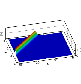
Figure 3: Evolution of the amplitude of the bright soliton with $k_{0}=2.0$.

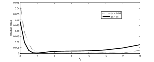
Figure 4: The reflection ratios when chosen different wavenumbers $k_{0}$ under mesh $\Delta x=0.1$ and its refinement mesh.

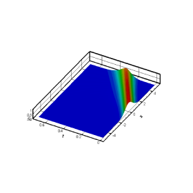
Figure 5: Evolution of the amplitude of the wave for the quintic NLS equation.

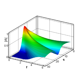
(a)      $k_{0}=1.75$ (b)  $k_{0}=2.0$

Figure 6: Evolution of the amplitude of matter wave with ABCs for different $k_{0}$.