Detrended fluctuation analysis of traffic data

Abstract

Different routing strategies may result in different behaviors of traffic on internet. We analyze the correlation of traffic data for three typical routing strategies by the detrended fluctuation analysis (DFA) and find that the degree of correlation of the data can be divided into three regions, i.e., weak, medium, and strong correlation. The DFA scalings are constants in both the regions of weak and strong correlation but monotonously increase in the region of medium correlation. We suggest that it is better to consider the traffic on complex network as three phases, i.e., the free, buffer, and congestion phase, than just as two phases believed before, i.e., the free and congestion phase.

Tel: 021-62233216(Office); 021-52705019(Home); 13585691004(Cell)
Fax:021-62232413
Email: zhliu@phy.ecnu.edu.cn

Undoubtedly, the internet has become a very important tool in our daily life. The operations on the internet, such as browsing World Wide Web (WWW) pages, sending messages by email, transferring files by ftp, searching for information on a range of topics, and shopping etc., have benefited us a lot. Therefore, sustaining its normal and efficient functioning is a basic requirement. However, the communication in the internet does not always march/go freely. Similar to the traffic jam on the highway, the intermittent congestion in the internet has been observed Huber:1997 . This phenomenon can be also observed in other communication networks, such as in the airline transportation network or in the postal service network. For reducing/controlling the traffic congestion in complex networks, a number of approaches have been presented arenas1:2002 ; moreno1:2003 ; moreno2:2004 ; moreno3:2004 ; zhao:2005 ; Liu:2006 ; Liu:2007 ; Yin:2006 ; Wang:2006 ; Echenique:2004 ; Echenique:2005 . Their routing strategies can be classified into two classes according to if the packets are delivered along the shortest path or not.

The delivering time of a packet from its born to its destination depends on the status of internet and the routing strategy. It is believed that there are two phases in communication, i.e., the free and congestion phase. In the routing strategy of the shortest path, the delivering time equals the path length in the free phase and become longer and longer in the congestion phase with time going. For the former, the delivering times for different packets will be uncorrelated as each individual packet can go freely to its destination; while for the later, they will become correlated as the waiting times are determined by the accumulated packets in their paths. In the routing strategy of non-shortest path, the delivering times may be different for different strategies even in the free phase. As the internet has a power-law degree distribution, the nodes with heavy links are easy to be the middle stations for packets to pass by and hence are easy to be congested. For reducing congestion on these heavy nodes, the packet may be delivered along a path which avoids the heavy nodes and hence the path is a little longer than the shortest path Echenique:2004 ; Echenique:2005 ; Liu:2006 ; Liu:2007 . Of course, the packets will still go the shortest path if the packets in the network is not accumulated. Therefore, it is possible for the delivering times to be either correlated or uncorrelated in the free phase. As the delivering times are closely related to the degree of accumulation of packets in the networks, the correlation of delivering times can be also reflected in the time series of packets of the network. A typical routing strategy of the shortest path is given by Liu et al. Liu:2006 . And two typical routing strategies of the non-shortest path are given by Echenique et al. Echenique:2004 ; Echenique:2005 and Zhang et al. Liu:2007 . Here we will study the correlation of packets produced by these three typical strategies.

As the traffic data are produced by all the nodes with some randomness, there exist erratic fluctuation, heterogeneity, and nonstationarity in the data. These features make the correlation difficult to be quantified. A conventional approach to measure the correlation in this situation is by the detrended fluctuation analysis (DFA), which can reliably quantify scaling features in the fluctuations by filtering out polynomial trends. The DFA method is based on the idea that a correlated time series can be mapped to a self-similar process by integration Peng:1994 ; Peng:1995 ; Liu:1999 ; Yang:2004 ; Chen:2005 . Therefore, measuring the self-similar feature can indirectly tell us information about the correlation properties. The DFA method has been successfully applied to detect long-range correlations in highly complex heart beat time series Peng:1995 , stock index Liu:1999 , and other physiological signals Chen:2005 . In this paper, we will use the DFA method to measure the correlation of traffic data.

Most of the previous studies assume that the creation and delivering rates of packets do not change from node to node. Considering the fact that different nodes in the internet have different capacities, a more realistic assumption is that the packet creation and delivering rates at a node are degree-dependent. This feature has been recently addressed by Zhao et al. zhao:2005 and Liu et al. Liu:2006 ; Liu:2007 . They assume that the creation and delivering rates of packets are $\lambda k_{i}$ and $(1+\beta k_{i})$, respectively, where $k_{i}$ is the degree of node $i$, $\lambda$ represents the ability of creating packets for a node with degree one, the $1$ in $(1+\beta k_{i})$ reflects the fact that a node can deliver at least one packet each time, and $\beta$ denotes the ability for a link to deliver packets. For a fixed $\lambda$, there is a threshold $\beta_{c}$. It is in the free phase when $\beta>\beta_{c}$ and in the congestion phase when $\beta<\beta_{c}$. Here we study how the scaling of correlation changes with the parameter $\beta$. We find that there is always a scaling in the DFA of traffic data and the scaling can be divided into three regions, which implies the existence of three phases of traffic on complex networks, i.e., the free, buffer, and congestion phase.

We now construct a scale-free network with the total number of nodes $N=1000$ and the average number of links connected with one node $<k>=6$ according to the algorithm given in Ref. LLYD:2002 and let every node create $\lambda k_{i}$ packets and send out at most $1+\beta k_{i}$ packets at each time step. The destinations of the created packets are randomly chosen and the sending out obeys the first-in-first-out rule. In the delivering process, the newly created and arrived packets will be placed at the end of the queues of each node. For the Liu’s approach of the shortest path, we follow the Ref. Liu:2006 to collect the time series of traffic data. Figure 1 shows the evolution of the average packets per node $<n(t)>$ in the network where the three lines from top to bottom represent the cases of $\beta=0.06<\beta_{c},\beta=0.061\approx\beta_{c}$, and $\beta=0.1>\beta_{c}$, respectively. Obviously, the packets in the congestion phase of $\beta=0.06$ increase linearly with time $t$, and the packets in the free phase of $\beta=0.061$ and $0.1$ fluctuate around different constants. For the Echenique’s approach of the non-shortest path, we follow the Ref. Echenique:2004 ; Echenique:2005 that a packet of node $i$ will choose one of its neighboring nodes, $\ell$, as its next station according to the minimum value of $\delta_{\ell}=hd_{\ell,j}+(1-h)n_{\ell}$, where $d_{\ell,j}$ is the shortest path length from the neighboring node $\ell$ to the destination $j$ and $n_{\ell}$ is the accumulated packets at node $\ell$. The parameter $h$ is a weighing factor, which can be taken as a variational parameter and $h\approx 0.8$ is found to give the best performance. The Echenique’s approach thus accounts for the waiting time only at the neighboring nodes. Echenique’s approach was presented for the case of equal creation and delivering rates at every node. For the delivery rate of $(1+\beta k_{i})$, a modified Echenique’s approach Liu:2007 is to choose a neighboring node with the minimum value of

$$\delta_{\ell}=hd_{\ell,j}+(1-h)\frac{n_{\ell}}{1+\beta k_{\ell}}.$$ (1)

We here choose $h=0.85$ in Eq.(1) and find that the traffic data has the similar behaviors for different $\beta$ as that shown in Fig. 1. And for the Zhang’s approach of the non-shortest path, we follow the Ref. Liu:2007 to collect the traffic data. For a packet at node $i$, we take a node $\ell$ from the neighbors of node $i$ and label the shortest path from node $\ell$ to the source $j$ by $\{SP:\ell,j\}$. Along this path, we evaluate the following quantity for the node $\ell$:

$$d(\ell)=\sum_{s\in\{SP:\ell,j\}}\frac{n_{s}}{1+\beta k_{s}},$$ (2)

where the sum is over the nodes along the shortest path $\{SP:\ell,j\}$, excluding the destination. Thus, $d(\ell)$ is an estimate of the time that a packet would take to go from node $\ell$ to the destination $j$ through the shortest path. The node $\ell$ with the minimum of $d(\ell)$ will be chosen as the next station of the packet at node $i$. We find that the traffic data also has the similar behaviors for different $\beta$ as that shown in Fig. 1.

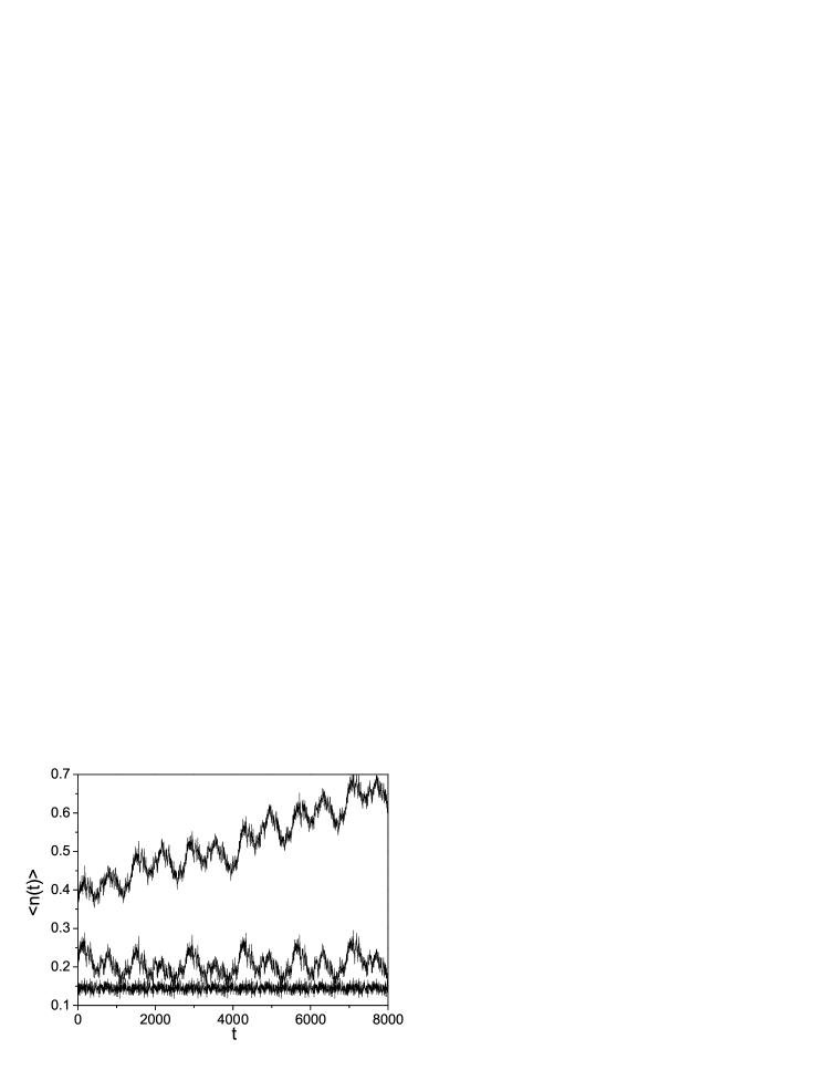
Figure 1: The average packets per node for $\lambda=0.01$ where the three lines from top to bottom represent the case of $\beta=0.06,0.061$, and $0.1$, respectively.

All the three typical approaches show a common feature that there are two kinds of data: the data in the congestion phase increases linearly with $t$ and the data in the free phase fluctuations around a constant. In order to quantify the correlations in the congestion phase, it is important to remove the global trend. Therefore, we remove the trend of linearly increasing with $t$ by subtracting a best fitting straight line of the time series. This procedure makes the data in congestion phase have the similar behavior with that in the free phase. Figure 2 shows an example of removing the global trend where the upper line denotes the original data with $\beta=0.06>\beta_{c}$ and the lower line the data after removing the global trend.

Figure 2: Removing the global trend of the congestion data for the shortest path approach where the upper line denotes the original data with $\beta=0.06>\beta_{c}$ and the lower line the data after removing the global trend.

The DFA method is a modified root-mean-square (rms) analysis of a random walk and its algorithm can be worked out as the following steps Peng:1994 ; Peng:1995 ; Liu:1999 ; Yang:2004 ; Chen:2005 :
(1) Start with a signal $s(j)$, where $j=1,\cdots,N$, and $N$ is the length of the signal, and integrate $s(j)$ to obtain

$$y(i)=\sum_{j=1}^{i}[s(j)-<s>],$$ (3)

where $<s>=\frac{1}{N}\sum_{j=1}^{N}s(j)$.
(2) Divide the integrated profile $y(i)$ into boxes of equal length $m$. In each box, we fit $y(i)$ to get its local trend $y_{fit}$ by using a least-square fit.
(3) The integrated profile $y(i)$ is detrended by subtracting the local trend $y_{fit}$ in each box:

$$Y_{m}(i)\equiv y(i)-y_{fit}(i).$$ (4)

(4) For a given box size $m$, the rms fluctuation for the integrated and detrended signal is calculated:

$$F(m)=\sqrt{\frac{1}{N}\sum_{i=1}^{N}[Y_{m}(i)]^{2}}.$$ (5)

(5) Repeat this procedure for different box size $m$.
For scale-invariant signals with power-law correlations, there is a power-law relationship between the rms fluctuation function $F(m)$ and the box size $m$:

$$F(m)\sim m^{\alpha}.$$ (6)

The scaling $\alpha$ represents the degree of the correlation in the signal: the signal is uncorrelated for $\alpha=0.5$ and correlated for $\alpha>0.5$ Peng:1994 ; Peng:1995 ; Liu:1999 ; Yang:2004 ; Chen:2005 .

We now use the DFA method to quantify the correlation and scaling properties of the fluctuated data with no global trend. For the collected data in the three typical approaches, Fig. 3 shows how the rms fluctuation function $F(m)$ changes with the scale $t$ where the lines from top to bottom in each panel denote the direction of increasing $\beta$ and (a) represents the case of Liu’s approach, (b) the case of Echenique’s approach, and (c) the case of Zhang’s approach. It is easy to see that all the lines are straight when $m$ is smaller than the crossover point (shown by the arrows), indicating there is a scaling $\alpha$ for each line. Comparing the the lines with different $\beta$, we see that the scaling $\alpha$ changes with $\beta$. The relationship between $\alpha$ and $\beta$ is shown in Fig. 4 where the lines with “squares”, “circles”, and “stars” denote the cases of Liu’s, Echenique’s, and Zhang’s approach, respectively.

Figure 3: $F(m)$ versus $m$ for different $\beta$ where the arrows show the crossover points, the dashed lines show the slopes/scalings of $F(m)$ for eye guide, and (a) represents the case of Liu’s approach, (b) the case of Echenique’s approach, and (c) the case of Zhang’s approach.

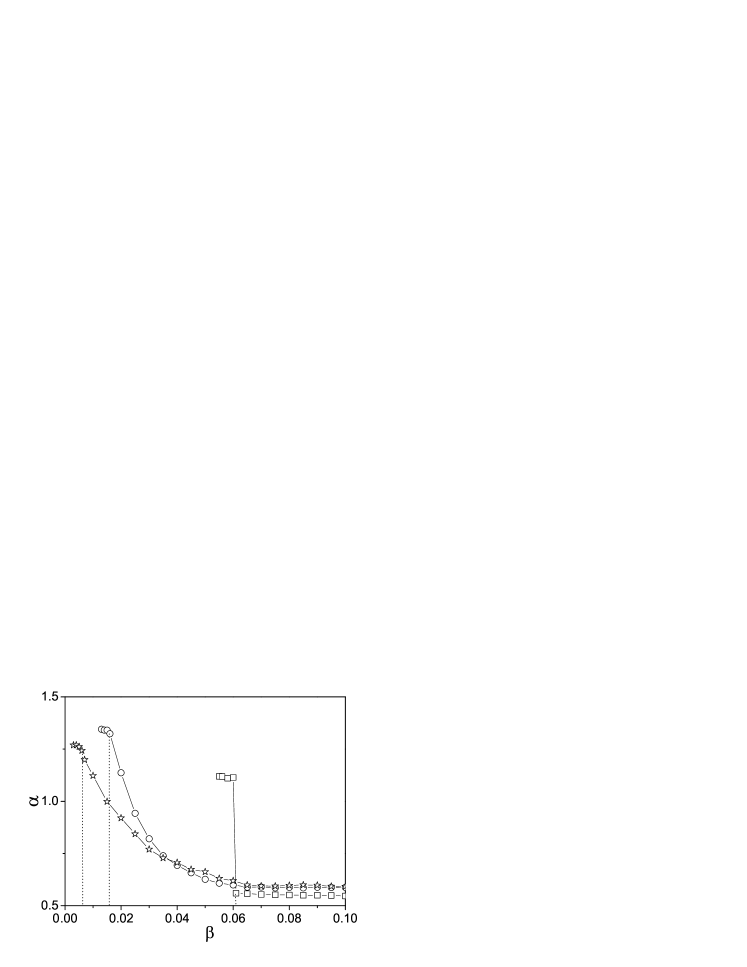
Figure 4: How the scaling $\alpha$ changes with $\beta$ where the lines with “squares”, “circles”, and “stars” denote the cases of Liu’s, Echenique’s, and Zhang’s approach, respectively, and the three dotted lines show the locations of $\beta_{c}$ for the three approaches.

From Fig. 4, it is easy to see that $\alpha$ is an approximate constant in the congestion phase ($\beta<\beta_{c}$) for all the three cases where $\beta_{c}$ are the locations of the three dashed lines, but $\alpha$ have different behaviors in the free phase between the method with the shortest path and that with the non-shortest path. In the Liu’s approach, $\alpha$ in the free phase is a constant, while in the Echenique’s and Zhang’s approaches, $\alpha$ is a constant for $\beta>0.061$ but monotonously increases before $\beta$ decreases to $\beta_{c}$. Let’s call the separation value of $\beta$ from a constant to increasing as $\beta_{1}$, namely $\beta_{1}=0.061$. Then, we have $\beta_{1}=\beta_{c}$ in Liu’s approach and $\beta_{1}>\beta_{c}$ in both the Echenique’s and Zhang’s approaches. For $\beta>\beta_{1}$, all the values of $\alpha$ are close to $0.5$, hence the corresponding traffic data are approximately uncorrelated. For $\beta_{c}<\beta<\beta_{1}$, the correlation in the Echenique’s and Zhang’s approaches are gradually increased from short range to long range correlation, and arrive global correlation for $\beta<\beta_{c}$. For distinguishing the three different behaviors, we call their corresponding traffic as free ($\beta>\beta_{1}$), buffer ($\beta_{c}<\beta<\beta_{1}$), and congestion ($\beta<\beta_{c}$) phase.

The relationship between the scaling $\alpha$ and the corresponding traffic behaviors can be understood as follows. In the strategy of the shortest path, as the accumulation of packets will firstly occur at the hub nodes, the network can be considered as congested once the hub nodes are congested Liu:2006 . In that time, there are no accumulated packets at the non-hub nodes. Hence, the critical value $\beta_{c}$ can be figured out by the average packets on the hub equalling $1+\beta_{c}k_{hub}$. Once the congestion occurs ($\beta<\beta_{c}$), the accumulation at the hub nodes will increase linearly and hence influence all the packets that take the hub nodes as the middle stations. As most of the shortest paths cross the hub nodes in scale-free networks, the influence of their congestion will be global and make a significant change in correlation when the traffic changes from free to congestion phase. This is why we observe the jump of $\alpha$ in the line with “squares” in Fig. 4.

While in the strategy of the non-shortest path, the accumulated packets at the hub nodes for $\beta_{c}<\beta<\beta_{1}$ will not increase linearly with time even when its average is slightly larger than $1+\beta k_{hub}$ because the coming packets will choose other paths to reduce the delivering time. Therefore, for a fixed creation rate, the packets will go longer and longer paths to avoid the congestion when the delivering parameter $\beta$ decreases. With the further decrease of $\beta$, more and more nodes have their average packets larger than $1+\beta k_{i}$, i.e., there are accumulated packets at these nodes. When the nodes with the smallest links begin to be accumulated with packets, the congestion occurs. Therefore, the correlation among the packets will become stronger and stronger with the decrease of delivering rate $\beta$. That is why we observe the gradually increase of $\alpha$ in the lines with “squares” and “circles” in Fig. 4. On the other hand, a packet will choose its path from all the nodes when $\beta<\beta_{c}$, thus the correlation will become global. And for $\beta>\beta_{1}$, the average packets at the hub nodes will not be over $1+\beta k_{hub}$, but the fluctuation of packets may be over $1+\beta k_{hub}$ sometimes. Once it happens, the coming packets will choose other paths to avoid the accumulation at the hub nodes, resulting a short range correlation even in the free phase. So we observe the “circles” and “stars” is a little higher than the “squares” for $\beta>\beta_{1}$ in Fig. 4. In sum, a difference between the buffer phase and the free phase is that the average packets on a node will be over $1+\beta k_{i}$ for the former but not for the later; and a difference between the buffer phase and the congestion phase is that the average packets on a node will increase linearly with time in the congestion phase but not in the buffer phase.

In conclusions, we have investigated the correlation of traffic data for three typical routing strategies by the DFA method. We find that there are two phases in the strategy of the shortest path but three phases in the strategy of the non-shortest path. The buffer phase comes from the fact that the coming packets will go a little longer paths with small nodes to avoid the heavy accumulation at the hub nodes. The average packets in the buffer phase is larger than that in the free phase but does not increase linearly with time. The finding of the buffer phase may shed light on the way of further studying the commulation in internet.

This work was supported by the NNSF of China under Grant No. 10475027 and No. 10635040, by the PPS under Grant No. 05PJ14036, by SPS under Grant No. 05SG27, and by NCET-05-0424.

References

- (1) Huberman B A and Lukose R M 1997 Science 277 535
- (2) Guimer R, Daz-Guilera A, Vega-Redondo F, Cabrales A and Arenas A 2002 Phys. Rev. Lett. 89 248701
- (3) Moreno Y, Pastor-Satorras R, Vazquez A and Vespignani A 2003 Europhys. Lett. 62 292
- (4) Echenique P Gomez-Gardenes J and Moreno Y 2004 cond-mat/0412053
- (5) Echenique P Gomez-Gardenes J and Moreno Y 2004 Phys. Rev. E 70 056105
- (6) Zhao L, Lai Y, Park K and Ye N 2005 Phys. Rev. E 71 026125
- (7) Yin C, Wang B, Wang W, Zhou T and Yang H 2006 Phys. Lett. A 351 220
- (8) Wang W, Wang B, Yin C, Xie Y and Zhou T 2006 Phys. Rev. E 73 026111
- (9) Liu Z, Ma W, Zhang H, Sun Y and Hui P 2006 Physica A 370 843
- (10) Echenique P, Gomez-Gardenes J and Moreno Y 2004 Phys. Rev. E 70 056105
- (11) Echenique P, Gomez-Gardenes J and Moreno Y 2005 Europhys. Lett. 71 325
- (12) Zhang H, Liu Z, Tang M and Hui P 2007 Phys. Lett. A 364 177
- (13) Peng C, Buldyrev S V, Havlin S, Simons M, Stanley H E and Goldberger A L 1994 Phys. Rev. E 49 1685
- (14) Peng C, Havlin S, Stanley H E and Goldberger A L 1995 Chaos 5 82
- (15) Liu Y, Gopikrishnan P, Cizeau P, Meyer M, Peng C and Stanley H E 1999 Phys. Rev. E 60 1390
- (16) Yang H, Zhao F, Qi L and Hu B 2004 Phys. Rev. E 69 066104
- (17) Chen Z, Hu K, Carpena P, Bernaola-Galvan P, Stanley H E and Ivanov P 2005 Phys. Rev. E 71 011104
- (18) Liu Z, Lai Y, Ye N and Dasgupta P 2002 Phys. Lett. A 303 337