Class of exactly solvable symmetric spin chains with matrix product ground states
Abstract
We introduce a class of exactly solvable symmetric Hamiltonians with matrix product ground states. For an odd case, the ground state is a translational invariant Haldane gap spin liquid state; while for an even case, the ground state is a spontaneously dimerized state with twofold degeneracy. In the matrix product ground states for both cases, we identify a hidden antiferromagnetic order, which is characterized by nonlocal string order parameters. The ground-state phase diagram of a generalized symmetric bilinear-biquadratic model is discussed.
pacs:
75.10.Pq, 75.10.Jm, 03.65.FdI Introduction
One-dimensional quantum Heisenberg antiferromagnets have a long history and show many fascinating properties. Since the Mermin-Wagner-Coleman theorem Mermin-1966 ; Coleman-1973 forbids a continuous symmetry breaking in one dimension, no classical Néel order can survive, even in zero temperature. The rigorous solutions on particular models provide essential insights to understand the properties of these quantum spin liquid states. For instance, the spin- antiferromagnetic Heisenberg chain has a Bethe-ansatz solution, Bethe-1931 ; Faddeev-1981 which yields a unique spin singlet ground state, gapless spin- excitations and power-law decay spin correlations. Meanwhile, additional next-nearest-neighbor interactions can frustrate the nearest-neighbor antiferromagnetic correlations. The Majumdar-Ghosh model Majumdar-1969 is such an exactly solvable example, which has a twofold-degenerate dimerized ground state, a finite-energy gap, and extremely short spin correlations.
Toward the quantum integer-spin models, Haldane gave a striking prediction that an excitation gap occurs between the ground state and the excited states. Haldane-1983 Although Haldane’s argument is based on a semiclassical large- expansion, it was later verified by numerical studies for lower- cases. Nightingale-1986 ; Takahashi-1989 ; White-1993 Remarkably, Affleck, Kennedy, Lieb, and Tasaki (AKLT) found a family of integer-spin chain Hamiltonians with exact massive ground states, which are called valence bond solid (VBS) states. Affleck-1987 The VBS states preserve spin rotational symmetry, and exhibit exponentially decay spin correlations and gapped excitations, thus, share the key features of Haldane gap spin liquid states for the quantum integer-spin Heisenberg antiferromagnets. Although no true long range order exists, den Nijs and Rommelse den Nijs-1989 observed a hidden antiferromagnetic order in the VBS state, and introduced a set of nonlocal string order parameters to provide a faithful quantification of the Haldane phase. The string order in VBS state, Haldane gap, and the fourfold degeneracy in an open chain can be understood by a hidden symmetry breaking. Kennedy-1991 ; Oshikawa-1992 ; Suzuki-1995 However, a nonlocal string order parameter that reflects correctly the hidden symmetry of the higher- VBS states remains an open problem. Oshikawa-1992 ; Suzuki-1995 ; Schollwock-1996 ; Tu-AKLT
Beside the studies on -symmetric spin chains, quantum spin systems with higher symmetry also attract much attention. For instance, the Bethe-ansatz method for Heisenberg chains can be generalized to models with symmetry. Sutherland-1975 It has been argued that such an -symmetric model can be achieved in electronic systems with two-fold orbital degeneracy at quarter filling. YQLi-1998 Meanwhile, Affleck et al. Affleck-1991 first discussed the extension of VBS states to -invariant extended VBS states, which break lattice translational symmetry and charge-conjugation symmetry but remain invariant under the combined operation of these two symmetries. Furthermore, Greiter et al. Greiter-2007 studied the spin chains with exact valence bond solid ground states. Along with the rise of cold atomic physics in optical lattices, Chen et al. YPWang-2005 constructed an Majumdar-Ghosh model with exact plaquette ground states by using spin- fermions. Very recently, Arovas Arovas-2008 explored a family of novel simplex solid states, which are natural generalizations of VBS states of AKLT models. Besides these models with symmetry, Schuricht and Rachel Rachel-2008 considered VBS states and their parent Hamiltonians.
In this paper, we will introduce a class of -symmetric Hamiltonians with matrix product states as their exact ground states. However, these symmetric spin chains show a different even-odd effect. For an odd , a periodic chain has a unique ground state. All these matrix product states have a hidden antiferromagnetic order, which is characterized by string order parameters. The nonlocal unitary transformations are designed to explicitly reveal a hidden symmetry. The breaking of this symmetry is responsible for the Haldane gap, nonvanishing string order parameters, and -fold degeneracy in an open chain. However, for an even , a periodic chain has a twofold dimerized ground state, which breaks translational symmetry. Nevertheless, these matrix product states also contain a hidden antiferromagnetic order. Finally, the ground-state phase diagram of a generalized symmetric bilinear-biquadratic model is obtained.
This paper is organized as follows. In Sec. II, the algebra and the exactly solvable symmetric models will be introduced. In Sec. III, the exact matrix product ground state of the model with will be studied, in particular, with the examples of and . The hidden order in all these matrix product states and the corresponding hidden symmetry are identified. Section IV is devoted to an analysis of the model with , which has a dimerized ground state breaking lattice translational symmetry. In Sec. V, a generalized symmetric bilinear-biquadratic model is introduced and their ground-state properties are discussed in detail. A conclusion is presented in Sec. VI.
II Model Hamiltonian
Let us begin with a one-dimensional chain of lattice sites ( even). On each site, the local Hilbert space contains states , which can be rotated within the space via the following vector relations:
| (1) |
where are the generators of the Lie algebra. The vector relations constitute the -dimensional representation of algebra and the following commutation relations hold: Georgi-1999
| (2) |
According to the Lie algebra, the tensor product of two vectors can be decomposed as a direct sum of an singlet with a dimension , an antisymmetric tensor with a dimension , and a symmetric tensor with a dimension , i.e.,
| (3) |
where the number above each underline is the dimension of the corresponding irreducible representation. For , we recover the well-known Clebsch-Gordan decomposition of two spin- representations. According to the decomposition scheme (3), the wave functions in each irreducible representation channel can be obtained explicitly. The maximally entangled singlet wave function is written as , and the wave functions of the antisymmetric channel are expressed as
| (4) |
Finally, the symmetric channel contains states with the wave functions
| (5) |
and the rest of states with the wave functions
| (6) |
For the three channels given in Eq. (3), the bond Casimir charge for two adjacent sites takes the values , , and , respectively. Together with the single-site Casimir charge , one can write the symmetric bilinear interaction term as a polynomial of bond projection operators,
| (7) | |||||
where the bond projectors , , and project the states of two adjacent sites and onto the three channels in Eq. (3), respectively. Using the property of projection operators, we square Eq. (7) and obtain the symmetric biquadratic interaction term as
| (8) | |||||
Combined with the completeness relation of the projectors,
| (9) |
we can express the bond projection operators with the generators as
| (10) | |||||
Now we define our model Hamiltonian as
| (11) |
which is a bilinear-biquadratic Hamiltonian in terms of the generators according to Eq. (10). This model has exact matrix product ground states, which will be extensively studied below. Although the exact excited states are not known, we argue that there is a finite energy gap above the ground states. For a projector Hamiltonian such as Eq. (11), this argument can be proved rigorously using a method proposed by Knabe, Knabe-1988 who found that the lower bounds of energy gaps of infinite systems can be obtained by diagonalizing finite-size systems.
In Secs. III and IV, we will discuss odd and even cases separately because the nature of the matrix product ground state depends on the parity of . Mathematically speaking, the and algebras are quite different. According to the Cartan classification scheme, Georgi-1999 the algebra belongs to type, while the algebra are type.
III Odd- case
Let us assume , where is an integer (). To achieve the exact ground state of model Hamiltonian (11), one has to resort to a fascinating property of algebra — the spinor representation. An elegant way to construct the spinor representation of algebra is to introduce gamma matrices satisfying the Clifford algebra . Then an irreducible spinor representation of is immediately constructed by . The product of and can be expressed as . For each lattice site , if the following matrix state is introduced:
| (12) |
then the bond product of at any two neighboring sites is given by
| (13) | |||||
where the first two terms belongs to the antisymmetric channel in Eq. (3) and the latter term is the singlet. Since performs the projection onto the states of the symmetric channel, the matrix product state defined by
| (14) | |||||
is always the zero energy ground state of the Hamiltonian (11) in a periodic boundary condition. This state preserves symmetry and lattice translational symmetry. For an open chain, there are totally -degenerate ground states, which can be distinguished by their edge states.
To compute the correlation functions in the matrix product ground state, we set up a transfer matrix method Klumper-1991 by introducing
| (15) |
where is an operator acting on a single site and denotes the complex conjugate of . Specifically, the transfer matrix is written as . Then a two-point correlation function in thermodynamic limit can be written as
| (16) |
where . In a long distant limit, the two-point correlation functions of generators decay exponentially as
| (17) |
with the correlation length .
Here we note that the symmetric model has a deep relation with the quantum integer-spin chains. On each lattice site, the vectors of can be constructed from the quantum spin states. In the spin language, the last two channels in Eq. (3) for odd correspond to the total bond spin and states, respectively. In other words, the bond projection operators can be expressed using the spin projection operators as
| (18) | |||||
| (19) |
Thus, the role of is to project onto nonzero even total spin states. Based on this property, we can further show that the matrix product wave function (14) is also the ground state of the following quantum integer-spin Hamiltonian:
| (20) |
with all . This model can be written as a polynomial of nearest neighbor spin exchange interactions up to powers and is therefore -invariant. However, the ground state (14) possesses an emergent symmetry.
It is interesting to compare with the AKLT model of valence bond solid proposed by Affleck et al., Affleck-1987 ; Arovas-1988
| (21) |
with all . The ground state of is also a matrix product state similar to Eq. (14), but the local matrix for AKLT model is now a matrix. Suzuki-1995 When , both models and become exactly the same as the AKLT model , whose ground state is the celebrated VBS state. When , we emphasis that and differ from each other. In Secs. III B and III C, we will show that their matrix product ground states have very different hidden structures and belong to different topological phases, although they both belong to the Haldane liquid states.
III.1 matrix product state: VBS
In order to investigate the property of the matrix product state, we briefly review the -symmetric VBS state as a warm up. In this case, the vectors can be represented by the spin states,
| (22) |
and the generators are defined by spin- operators as and . Moreover, the Clifford algebra is satisfied by the Pauli matrices as . According to Eq. (12), the local matrix can be written as
| (23) |
which generates the matrix form of the VBS state. Although the two-point spin-correlation functions in this state decay exponentially as shown in Eq. (17), it has been observed that the upper and down spins lie alternately along the lattice, sandwiched by arbitrary number of non-polarized spin states. This hidden diluted antiferromagnetic order can be characterized by a nonlocal string order parameter first proposed by den Nijs and Rommelse, den Nijs-1989
| (24) |
where , , or .
On the other hand, the VBS states on a finite open chain have two nearly free edge degrees of freedom at the end of the chain and are thus fourfold degenerate. Both the hidden string order and the degeneracy in an open chain can be understood as natural consequences of a hidden symmetry breaking. To manifest the hidden symmetry, the key is a nonlocal unitary transformation defined by Kennedy-1991 ; Oshikawa-1992
| (25) |
In the standard representation, flips to and multiplies the state with a phase factor . The physical meaning of the unitary transformation can be explained as follows. For a given spin configuration on a finite open chain, all are left alone and we look for the non-zero spins from the left to the right. Suppose there is a non-zero spin at site , we count the number of and on the sites to the left of site . If the number is even, we left the spin at site unchanged. If the number is odd, we flip the -site spin. Finally, an additional phase factor may be taken into account, depending on the total site number and each spin configuration. An example of the unitary transformation on a typical configuration of the spin- VBS state is shown in Fig. 1.
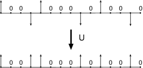
When applying the Kennedy-Tasaki unitary transformation to the Hamiltonian, the -symmetric AKLT model is transformed to a model with a discrete symmetry, Kennedy-1991 ; Oshikawa-1992 and two of the den Nijs-Rommelse string order parameters become the usual two-point spin-correlation functions. Thus, the nonvanishing string order parameter measures the hidden symmetry breaking of the original model. The breaking of this hidden discrete symmetry leads to the opening of the Haldane gap, the hidden antiferromagnetic order, and the fourfold degeneracy in an open chain and thus provides a unified explanation of the exotic features in VBS states.
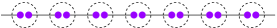
III.2 matrix product state: A projected valence bond solid
The next example is the -symmetric matrix product state with . Actually, Scalapino et al. Scalapino-1998 proposed this state to describe the “superspin” phase on a ladder system of interacting electrons. Here, it is convenient to introduce the vectors by means of the states,
| (26) |
Moreover, we define the gamma matrices as
| (27) |
Then the local matrix can be written as
| (28) |
In fact, the matrix product state can be interpreted as a projected VBS state (Fig. 2). By using two spin- fermions, the spin- states can be constructed as Wu-2003 ; Tu-2006
| (29) |
where creates a fermion with spin components . Because only site quintet () and site singlet () are allowed for two spin- fermions on a single site, an extra projection has to be implemented to remove the site-singlet state. Owing to , there exists an antisymmetric matrix with the following properties:
| (30) |
Using the matrix, the matrix product state in a periodic chain can be written in a projected VBS wave function as
| (31) |
where is the site-quintet projector and is an -invariant valence bond singlet. For an open boundary condition, the chain is ended with two nearly free spin- degrees of freedom leading to degenerate ground states. Here we recall that the edge states of the VBS states of the AKLT model are spin- degrees of freedom, which are sharply different from our matrix product states.
Similar to the spin- VBS state, the matrix product states have an interesting hidden string order. Since the algebra is rank , one can classify the states by using two quantum numbers (weights) corresponding to the mutual commuting Cartan generators and as
| (32) |
These states, characterized by the weights, are related to those states denoted by the usual quantum numbers as follows:
| (33) |
When we define
| (34) |
the local matrix in Eq. (28) can be rewritten as
| (35) | |||||
By considering the property of Clifford algebra, it can be found that and must appear alternately in the matrix product states despite arbitrary numbers of and between them. At the same time, and also appear alternately with arbitrary numbers of and between them. For example, a typical configuration of the matrix product state is
where represent . This dilute antiferromagnetic order is in analogy with the spin- valence bond solid (VBS) state in terms of the quantum number, but here two quantum numbers are associated with the Cartan generators and . However, such an intriguing feature is not enjoyed by the VBS states of Affleck, Kennedy, Lieb, and Tasaki (AKLT) model. Actually, the characterization scheme of the VBS states for remains a challenging open problem. However, the hidden order of all matrix product states can be fully identified in a systematic and compact form.
III.3 Hidden order in the matrix product state
Now we are in a position to identify the hidden order in all the matrix product state (14), which is inspired from the analysis of matrix product state. Since is a rank- algebra, one can always choose the mutually commuting Cartan generators as . At each site, the quantum states are classified by the eigenvalues of these Cartan generators as
| (36) |
Thus, the single-site states are associated with quantum numbers and they are subjected to the constraint
| (37) |
According to Eq. (1), all the Cartan generators annihilate the “extra dimension” vector . The other basis states can be chosen as
| (38) |
From the property of the Clifford algebra, the hidden antiferromagnetic order of the ground state can now be identified. In any of the channel, it can be shown that is diluted antiferromagnetically ordered, the same as for the VBS state. Namely, the states of and will alternate in space if all the states between them are ignored.
This hidden antiferromagnetic order can also be characterized by nonlocal string order parameters. Similar to the case, the string order parameters can be defined as
| (39) |
Since the ground state is rotationally invariant, the above nonlocal order parameters should all be equal to each other. Thus, to determine the value of these parameters, only needs to be evaluated. One can compute the value of these string order parameters by the transfer-matrix techniques but there is an alternate intuitive approach. In the channel, the role of the phase factor in Eq. (39) is to correlate the finite spin-polarized states in the channel at the two ends of the string. If nonzero takes the same value at the two ends, then the phase factor is equal to . On the other hand, if nonzero takes two different values at the two ends, then the phase factor is equal to . Thus, the value of is determined purely by the probability of appearing at the two ends of the string. It is straightforward to show that the probability of the states appearing at one lattice site is and thus .
In the Lie algebra, , , and span an sub-algebra in which plays the role of flipping the quantum number . This exponential operator can flip the quantum numbers of without disturbing the quantum states in all other channels. This indicates that if we take the following nonlocal unitary transformation in the channel:
| (40) |
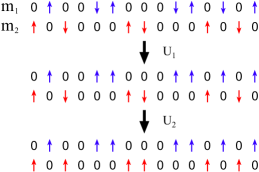
then all the configurations in this channel will be ferromagnetically ordered. Furthermore, by performing this nonlocal transformation successively in all the channels,
| (41) |
then all the configurations of the ground state will become ferromagnetically ordered. As an example, Fig. 3 shows how a typical configuration of the matrix product state is successively changed under this nonlocal unitary transformation.
By applying the unitary transformation (41) to the Cartan generators, it can be shown that
| (42) |
Substituting this formula to Eq. (39), we find that
| (43) |
Thus, the nonlocal string order parameters for Cartan generators become the ordinary two-point correlation functions of local operators after the unitary transformation.
Under the above transformation, the symmetry of the original Hamiltonian is reduced and determined by the symmetry of the unitary transformation operators. In the channel, it can be shown that the unitary operator possesses only a symmetry. Therefore, the Hamiltonian after the transformation has a symmetry. This is the hidden topological symmetry of the Hamiltonian, associated with the hidden order of the original matrix product state . When it is applied to an open chain system, the hidden topological symmetry of the Hamiltonian will be further broken, yielding -free edge states at each end of the chain. Therefore, the open chain has totally -degenerate ground states, which can be distinguished by their edge states.
IV Even- case
Let us assume . Using the gamma matrices, the spinor representation of the algebra can be constructed by leaving out . However, we note that the resulting -dimensional spinor representation generated by is reducible, in contrast to the algebra. Georgi-1999 Since commutes with all the generators , one can construct the following projection operators onto two different invariant subspaces:
| (44) |
For each lattice site , we introduce the local matrix as
| (45) |
then the exact matrix product ground states of the Hamiltonian (11) for are given by
| (46) | |||||
Due to the equation , we can observe that the states are dimerized states and are connected to each other by translating one lattice site. Thus these two states break translational symmetry while they preserve the rotational symmetry. For an open chain, the matrix product ground states are -fold degenerate when combining dimerization and edge states.
The static correlation functions can be computed by the transfer-matrix method as well. We find that the matrix product states have only nearest-neighbor correlations and the correlation length is zero. For , the two-point correlation function has an exponential tail at a large distance, as in Eq. (17), and the correlation length is .
Although these two-point correlation functions of the matrix product states are short range, there is a hidden antiferromagnetic order, similar to the matrix product states. Because is a rank- algebra, the Cartan generators can be chosen as . Thus, the states can be characterized by the weight using Eq. (38). In the case, the only difference is the absence of the extra dimension vector annihilated by all Cartan generators. To measure this hidden order, one can use the string order parameter in Eq. (39). A straightforward calculation shows the value of these string order parameters that are given by
| (47) |
Here we note that translational symmetry breaking distinguishes the case from the case, while the latter belongs to the Haldane spin liquid class. This is an interesting even-odd effect. Furthermore, one may expect that their low-lying excitations are also very different. The low-energy excitations in the Haldane liquid are magnons, while the systems are soliton-like excitations connecting the two dimerized states. Although the exact results of the low-lying excitations do not exist, more evidence comes from the case.
IV.1 SO(4) matrix product state: A staggered spin-orbital crystal
The case is somewhat special because it can be factorized as with being its vector representation. Namely, one can consider a spin-orbital coupled chain or equivalently a spin- two-leg spin ladder to implement the vectors and generators in Eq. (1). We find that it is convenient to introduce the four vector states as
| (48) |
where the first index in denotes the spin direction while the second one is the orbital direction. Moreover, the generators are defined by
| (49) |
where and , , or denote the spin and orbital degrees of freedom, respectively. Alternately, and can be viewed as the spin operators in the upper and lower leg of a two-chain ladder.
A convenient choice of matrices for spinor representation is given by
| (50) |
The invariant subspace projector is and . A little calculation shows that the local matrix is given by
| (51) |
up to an unimportant normalization factor.
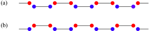
In this case, the twofold-degenerate ground states have an intuitive meaning, which becomes clear when the local Hilbert space is represented by a Schwinger-boson Fock space as . Here and create a state with spin and orbital directions and , respectively. Using these Schwinger bosons, we find that the state in Eq. (46) can be written as
| (52) | |||||
and the interchange of and yields . These staggered spin-orbital crystal states are first found by Kolezhuk and Mikeska. Kolezhuk-1998 The picture of these states is displayed in Figs. 4(a) and 4(b). Obviously, the two-point correlation functions are nonvanishing only between nearest-neighbor sites. For this spin-orbital system, the string order parameters in Eq. (47) can be written as
| (53) |
where , , or . In the studies of two-leg spin ladders, these types of string order parameters were introduced to divide the topologically distinct gapped spin liquid states. EHKim-2000
The fact that such two dimerized states are exact ground states of the projector Hamiltonian (11) can be easily visualized when writing the projectors of the three channels in Eq. (10) as
| (54) |
where and are bond total spin projectors. Once the spin and orbital singlets are formed between nearest-neighbor sites in a staggered pattern, the -symmetric projector Hamiltonian,
| (55) | |||||
always annihilate such a spin-orbital crystal state.
V bilinear-biquadratic model
As already mentioned, is a bilinear-biquadratic Hamiltonian in terms of the generators. More generally, we can also introduce a one-parameter family of the symmetric bilinear-biquadratic model,
| (56) |
which is an extension of the familiar spin- bilinear-biquadratic model. The absence of the higher-order terms follows from the fact that such terms can be expressed via the lower-order terms by means of Eq. (10). To sketch the properties of this bilinear-biquadratic model, we need to identify several special integrable points. Let us introduce a slave boson representation,
| (57) |
which yields a constraint . Using the slave bosons, the generators can be written as , and the -singlet bond projector in Eq. (10) is given by
| (58) |
Additionally, the -invariant permutation operator is expressed as
| (59) |
Using the permutation operator and the singlet projector, we can express the bilinear-biquadratic Hamiltonian (56) as
| (60) | |||||
up to a constant. Several special points can be identified as follows:
(1) and ; the Hamiltonian (56) reduces to a sum of nearest-neighbor permutation operators, thus, it has an enhanced symmetry. In this case, the transformation on each lattice site is in the fundamental representation. For , this is the Uimin-Lai-Sutherland (ULS) model, Sutherland-1975 which can be solved by Bethe-ansatz method. It is known that there are gapless excitations above the ground states and the effective low-energy field theory is described by an Wess-Zumino-Witten model. Affleck-1986
(2) ; the Hamiltonian (56) reduces to a sum of nearest-neighbor singlet projectors and also has an symmetry. However, the transformations are in the fundamental and its conjugate representations on the even and odd numbers of lattice sites, respectively. For , a mapping to the -state quantum Potts model allows the model to be solved exactly, Parkinson-1987 ; Barber-1989 ; Klumper-1989 and the ground states are dimerized states with a finite-energy gap.
(3) ; the Hamiltonian (56) was exactly solved by Reshetikhin Reshetikhin-1983 via quantum inverse scattering method, which also exhibited gapless excitations. For , this point corresponds to the spin- Takhatajan-Babujian model, Takhatajan-1982 which is the quantum critical point between Haldane gap phase and dimerized phase. For , the Reshetikhin point yields the Heisenberg model, which is equivalent to two decoupled spin- Heisenberg antiferromagnetic spin chains.
(4) ; the ground states of the model Hamiltonian (56) are just the matrix product states considered in Secs. III and IV. For an odd , the ground state is a unique Haldane liquid state. For an even , the ground states are twofold-degenerate dimerized states and are referred to non-Haldane liquid states.
Therefore, these rigorous results suggest that an energy gap develops for the model (56) in the finite parameter region
| (61) |
which always includes our matrix product ground-state point . The gap formation in this region is quite subtle. In the point of view of conformal field theory, the ULS and the Reshetikhin points are both conformal invariant and are characterized by two effective-field theories with different central charges. If so, there will be no renormalization flow from the Reshetikhin point to the -symmetric point according to Zamolodchikov’s theorem, Zamolodchikov-1986 and an energy gap must be generated between these two conformal invariant points. It was known that the conformal field theory for the ULS point is an Wess-Zumino-Witten model with central charge . The conformal field theory description for the Reshetikhin point is an Wess-Zumino-Witten model with central charge . In particular, the Takhatajan-Babujian model is known to have a central charge and the Heisenberg model (two decoupled spin- Heisenberg antiferromagnetic spin chains) has a central charge .
Toward the odd case, Itoi and Kato Itoi-1997 found that a marginally relevant perturbation around the ULS point develops a Haldane gap for , while the region near the ULS point is massless. However, the even case was extensively studied for , which corresponds to an spin-orbital coupled system. Nersesyan-1997 ; Pati-1998 ; Azaria-1999 ; Itoi-2000 ; GMZhang-2003 These results reveal that there is a dimerized non-Haldane liquid phase with an energy gap between the -symmetric point and the Heisenberg point. In the non-Haldane liquid state, magnon excitations are incoherent and the low-energy excitations are a pair of solitons connecting two spontaneously dimerized ground states. It is thus expected that these symmetric models also show such an interesting even-odd effect not only in the ground states but also in the low-energy excitations. For , the system is in a Haldane gap liquid phase with magnon excitations. For , the elementary excitations are solitons connecting the degenerate ground states.
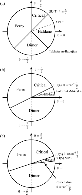
Following the exact results, the main phase diagrams of bilinear-biquadratic model for are displayed in Fig. (5). However, the antiferromagnetic Heisenberg model deserves more attention, corresponding to the bilinear-biquadratic model (56) with a pure bilinear interaction for . When , it is just the quantum spin- antiferromagnetic Heisenberg model, which is in the Haldane gap region. When , the Heisenberg model is equivalent to two decoupled spin- antiferromagnetic chains, which have unique disordered ground states with power-law decay spin correlations. However, when , we find that the antiferromagnetic Heisenberg model is not included in the Haldane gap region. Therefore, it is interesting to ask what are the ground states of the antiferromagnetic models for . Based on a generalized Lieb-Schultz-Mattis theorem, Li YQLi-2001 studied antiferromagnetic models for . He found that the Heisenberg model is gapless, while and Heisenberg models are suspected to have a gap. Together with our results, we predict that the Heisenberg model for belongs to the dimerized phase with a finite-energy gap.
VI Conclusion
In conclusion, we have introduced a class of symmetric spin chain Hamiltonians with nearest-neighbor interactions, whose exact ground states are two different symmetric matrix product states depending on the parity of .
For an odd , a periodic chain has a unique ground state, which preserves an rotational and translational symmetries. The symmetric spin chains with different are directly related to quantum integer-spin chains belonging to the Haldane gap phase with a hidden antiferromagnetic order characterized by nonlocal string order parameters. The hidden symmetry responsible for the hidden order has been found by applying a unitary transformation to the model Hamiltonian. The Haldane gap and degenerate ground states in an open chain are natural consequences of this hidden symmetry breaking.
For an even , a periodic chain has a twofold-degenerate dimerized ground state, which preserves symmetry but breaks translational symmetry. These matrix product states with different are non-Haldane liquid states, which have soliton excitations connecting the two degenerate ground states. However, these matrix product states also contain a hidden antiferromagnetic order characterized by nonlocal string order parameters.
Finally, a generalized symmetric bilinear-biquadratic model family has been discussed and the ground-state phase diagrams are sketched based on some known exact results. One of the important conclusions is that the ground state of the symmetric Heisenberg antiferromagnetic spin model for is predicted to be in a twofold-degenerate dimerized state. Further investigations on this are certainly required.
We acknowledge the support of NSF of China and the National Program for Basic Research of MOST-China.
References
- (1) N. D. Mermin and H. Wagner, Phys. Rev. Lett. 17, 1133 (1966).
- (2) S. Coleman, Commun. Math. Phys. 31, 259 (1973).
- (3) H. Bethe, Z. Phys. 71, 205 (1931).
- (4) L. D. Faddeev and L. A. Takhtajan, Phys. Lett. 85A, 375 (1981).
- (5) C. K. Majumdar and D. K. Ghosh, J. Math. Phys. 10, 1388 (1969); J. Math. Phys. 10, 1399 (1969); C. K. Majumdar, J. Phys. C 3, 911 (1970). P. M. van den Broek, Phys. Lett. 77A, 261 (1980).
- (6) F. D. M. Haldane, Phys. Lett. 93A, 464 (1983); Phys. Rev. Lett. 50, 1153 (1983).
- (7) M. P. Nightingale and H. W. Blöte, Phys. Rev. B 33, 659 (1986).
- (8) M. Takahashi, Phys. Rev. Lett. 62, 2313 (1989).
- (9) S. R. White and D. A. Huse, Phys. Rev. B 48, 3844 (1993).
- (10) I. Affleck, T. Kennedy, E. H. Lieb and H. Tasaki, Phys. Rev. Lett. 59, 799 (1987); Commun. Math. Phys. 115, 477 (1988).
- (11) M. den Nijs and K. Rommelse, Phys. Rev. B 40, 4709 (1989).
- (12) T. Kennedy and H. Tasaki, Phys. Rev. B 45, 304 (1992); Commun. Math. Phys. 147, 431 (1992).
- (13) M. Oshikawa, J. Phys.: Condens. Matter 4, 7469 (1992).
- (14) K. Totsuka and M. Suzuki, J. Phys.: Condens. Matter 7, 1639 (1995).
- (15) U. Schollwöck, O. Golinelli, and T. Jolicœur, Phys. Rev. B 54, 4038 (1996).
- (16) H. H. Tu, G. M. Zhang, and T. Xiang, arXiv:0807.3143.
- (17) G. V. Uimin, JETP Lett. 12, 225 (1970); C. K. Lai, J. Math. Phys. 15, 1675 (1974); B. Sutherland, Phys. Rev. B 12, 3795 (1975).
- (18) Y. Q. Li, M. Ma, D. N. Shi, and F. C. Zhang, Phys. Rev. Lett. 81, 3527 (1998).
- (19) I. Affleck, D. P. Arovas, J. B. Marston, and D. A. Rabson, Nucl. Phys. B 366, 467 (1991).
- (20) M. Greiter, S. Rachel, and D. Schuricht, Phys. Rev. B 75, 060401(R) (2007); M. Greiter and S. Rachel, Phys. Rev. B 75, 184441 (2007).
- (21) S. Chen, C. Wu, S. C. Zhang, and Y. P. Wang, Phys. Rev. B 72, 214428 (2005).
- (22) D. P. Arovas, Phys. Rev. B 77, 104404 (2008).
- (23) D. Schuricht and S. Rachel, Phys. Rev. B 78, 014430 (2008).
- (24) H. Georgi, Lie algebras in Particle Physics (Perseus Books, Reading, MA, 1999).
- (25) S. Knabe, J. Stat. Phys. 52, 627 (1988).
- (26) A. Klümper, A. Schadschneider, and J. Zittartz, J. Phys. A 24, L955 (1991); Z. Phys. B: Condens. Matter 87, 281 (1992).
- (27) D. P. Arovas, A. Auerbach, and F. D. M. Haldane, Phys. Rev. Lett. 60, 531 (1988).
- (28) D. Scalapino, S. C. Zhang, and W. Hanke, Phys. Rev. B 58, 443 (1998);
- (29) C. Wu, J. P. Hu, S. C. Zhang, Phys. Rev. Lett. 91, 186402 (2003).
- (30) H. H. Tu, G. M. Zhang, and L. Yu, Phys. Rev. B 74, 174404 (2006); Phys. Rev. B 76, 014438 (2007).
- (31) A. K. Kolezhuk and H. J. Mikeska, Phys. Rev. Lett. 80, 2709 (1998).
- (32) E. H. Kim, G. Fáth, J. Sólyom, and D. J. Scalapino, Phys. Rev. B 62, 14965 (2000); G. Fáth, Ö. Legeza, and J. Sólyom, Phys. Rev. B 63, 134403 (2001).
- (33) I. Affleck, Nucl. Phys. B 265, 409 (1986).
- (34) J. B. Parkinson, J. Phys. C 20, L1029 (1987); ibid. 21, 3793 (1988).
- (35) M. N. Barber and M. T. Batchelor, Phys. Rev. B 40, 4621 (1989); M. T. Batcherlor and M. N. Barber, J. Phys. A 23, L15 (1990).
- (36) A. Klümper, Europhys. Lett. 9, 815 (1989); J. Phys. A 23, 809 (1990).
- (37) N. Y. Reshetikhin, Lett. Math. Phys. 7, 205 (1983); Theor. Math. Phys. 63, 555 (1985).
- (38) L. A. Takhatajan, Phys. Lett. 87A, 479 (1982); H. M. Babujian, ibid. 90A, 479 (1982).
- (39) A. B. Zamolodchikov, JETP Lett. 43, 730 (1986).
- (40) C. Itoi and M. H. Kato, Phys. Rev. B 55, 8295 (1997).
- (41) A. A. Nersesyan and A. M. Tsvelik, Phys. Rev. Lett. 78, 3939 (1997).
- (42) S. K. Pati, R. R. P. Singh, and D. I. Khomskii, Phys. Rev. Lett. 81, 5406 (1998).
- (43) P. Azaria, A. O. Gogolin, P. Lecheminant, and A. A. Nersesyan, Phys. Rev. Lett. 83, 624 (1999); P. Azaria, E. Boulat, and P. Lecheminant, Phys. Rev. B 61, 12112 (2000).
- (44) C. Itoi, S. Qin, and I. Affleck, Phys. Rev. B 61, 6747 (2000).
- (45) G. M. Zhang, H. Hu, and L. Yu, Phys. Rev. B 67, 064420 (2003).
- (46) Y. Q. Li, Phys. Rev. Lett. 87, 127208 (2001).