Anderson localization: 2-D system in an external magnetic field

Abstract

The analytical approach developed by us for the calculation of the phase diagram for the Anderson localization via disorder [J.Phys.: Condens. Matter 14, 13777 (2002)] is generalized here to the case of a strong magnetic field when $q$ subbands ($q=1,2,3$) arise. It is shown that in a line with the generally accepted point of view, each subband is characterized by a critical point with a divergent localization length $\xi$ which reveals anomaly in energy and disorder parameters. These critical points belong to the phase coexistence area which cannot be interpreted by means of numerical investigations. The reason for this is a logical incompleteness of the algorithm used for analysis of a computer modelling for finite systems in the parameter range where the finite-size scaling is no longer valid.

1 Introduction

In the series of our recent papers [1, 2, 3, 4, 5] an exact analytic solution for the Anderson localization [6] was presented. As it has been commented [7, 8, 9], most of our results contradict the generally-accepted rules of the scaling theory and numerical modelling. Two particular results were highly unexpected in the Anderson community: (i) existence of the Anderson transition in two dimensional (2-D) disordered systems of noninteracting electrons, and (ii) the Anderson transition in N-D ($N\geq 2$) dimensions is of first-order, and localized and conducting states could co-exist.

The result (i) formally does not contradict experiment [10], where the unexpected presence of a metallic phase in 2-D was observed [11]. It was noted [10] that experiments of the last decade do not support the prevailing point of view that there can be no metallic state or metal-insulating transition in a 2-D system. The physics behind these observations at present is not understood.

The problem is that the experimental facts present not a strong argument for many theoreticans who believe that they are able to calculate disordered systems of noninteracting electrons [12]. This problem was studied in the literature by various methods: scaling theory of localization, perturbation theory, numerical modelling, etc. The conclusion has been drawn (but not proved) that a phase transition in experimental systems is related most likely to the interactions (Coulomb, spin-orbit) neglected in theory. However, this statement is valid only for theoretical Hamiltonian-based methods. In particular, the scaling theory of localization [13] is a phenomenological approach and thus could potentially be able to take into account strong particle interactions. The fact that this theory [13] is unable to describe experimental data indicates its serious problems. It is also possible that a 2-D metal-insulator transition is also possible for noninteracting electrons [1, 8]; however, existing theoretical methods are not suited for solving such a complex problem.

It should be also noted here that the above-mentioned consensus that in 2-D all states are localized should be reconsidered in the light of the conflicting situation. Indeed, as it was noted in a recent review article [12] devoted to the numerical investigations of the Anderson localization, practically all numerical results are in contradiction with the analytical predictions (see also discussion in Ref.[14]). Despite author [12] claims that results of numerical analysis could be treated as obtained “from first principles”, one should remember that any numerical analysis is based on certain analytical predictions. In particular, the necessity to modify the numerical algorithm for finite-size scaling was discussed [8]. The applicability of finite-size scaling studies has also been questioned [15, 16]. In other words, there is an obvious conflict between the results of different analytical and numerical methods.

This is why instead of the discussing point (i) [existence vs nonexistence of 2-D phase transition] it is more reasonable to consider consequences of point (ii) in the light of the applicability of finite-size scaling. This is important since this is a key method in both numerical investigations of the Anderson localization [12] and analytical realization of the finite-size scaling [8]. The concept of a finite-size scaling is taken from theory of phase transitions [17, 18, 19], and in fact is based on the extrapolation of the results for finite-size systems (length $L<\infty$) for the thermodynamic limit, $L=\infty$. It is clear that as the result of such an extrapolation, a single limiting value should be obtained. However, this is true only for the second-order phase transitions and in fact, the finite-size scaling [17, 18, 19] could be applied only to this particular case, but not to the theory of phase transitions in general.

This leads usually to the assumption of the existence of the correlation length which is divergent at the critical point [12]. The method cannot be used for the first-order transitions with a known multiplicity of solutions [1, 3, 5] where for an arbitrary set of system parameters two phases can coexist (localized and delocalized in our case). As mentioned in Ref. [1], a trivial example is the phase co-existence of ice and water. Only properties of the two pure homogeneous phases are physically meaningful, whereas an extrapolation of the results for a heterophase system has no real meaning. However, when the result of finite-size scaling do not fit to the second-order transition, the quick (and wrong) conclusion is often drawn that no phase transition occurs at all [1] neglecting a possibility of the first-order transition.

The type of the phase transition does not follow from any first-principles [20] and should not be the matter of speculations [14]. This is defined by the exact solution (if it exists) or careful analysis of information taking into account all possible alternatives. From the experimental point of view, the first-order phase transitions are observed relatively easily. In particular, the direct electrostatic probing [21] and photoluminescence spectroscopy [22] clearly show co-existence of localized and metallic regions associated with 2-D metal-insulating transition. New theories are put forward to address this issue[23, 24].

In the present paper, we apply our approach [1, 2, 3, 4, 5] to a 2-D system in an external magnetic field. The field could be included into a 2-D Hamiltonian by means of a Peierls factor [12]. This model is used for numerical analysis of the critical Hall regime in disordered systems in a strong perpendicular magnetic field. The prevailing viewpoint for this model is that no metal-insulator transition can occur here. It is believed also that there is the critical energy $E_{c}$ in each Landau band at which electrons are delocalized [25]. In other words, this is nothing but a generalization of our dispute on phase transitions [1, 2, 3, 4, 5] for the case of an external magnetic field. We demonstrate below that the model can be exactly solved using the analytical approach [1, 2, 3] for a certain range of magnitude of the control parameter (magnetic flux). As a result, the generally-accepted viewpoint on the metal-insulator transitions should be revised. Moreover, unlike the standard opinion [25] that the delocalization at the critical energy $E_{c}$ arises entirely due to a strong magnetic field, we show below that the existence of phase transitions without magnetic field and the critical energy $E_{c}$ in the magnetic field are mutually related.

Note that under the exact solution in this paper we mean only the calculation of the phase diagram with the localization length. To solve this problem, we use the recursive equation for the Cauchy problem with fixed initial conditions. There are some limitations of the analytical theory. An exact solution is only possible for the conventional Anderson model with a diagonal disorder, where on-site potentials are independently and identically distributed. We do not calculate here transport and other (energy spectrum, etc) properties, which corresponds to the problem with fixed boundary conditions (the Dirichlet problem) and has no exact solution.

The paper is organized as follows. In Section 2 the Schrödinger equation is discussed for noninteracting particles in the presence of a perpendicular magnetic field. The calculation of the joint correlators is discussed which permits to extract analytically information on the Lyapunov exponents and to draw the phase diagram. Since we extend our approach [1, 2, 3] for the case of magnetic field, we discuss mostly the necessary modifications of our approach. This is why knowledge of our previous papers is prerequisite here. The Lyapunov exponents are found using theory of functions of complex variables (via search of poles of the $H(z)$ function on the complex plane). Two conformal mappings are discussed in Section 3 which permit us to reduce the pole search to a relatively simple algebraic problem. In Section 4 the main results are summarized and nontrivial aspects of our theory analyzed.

2 Main definitions

2.1 The model

We consider a single-band disordered Anderson tight-binding model with Schrödinger equation [12]

$$\psi_{l+1,m}+\psi_{l-1,m}+\exp(-ik_{0}l)\psi_{l,m+1}+\exp(ik_{0}l)\psi_{l,m-1}=(E-\varepsilon_{l,m})\psi_{l,m}$$ (1)

describing the properties of noninteracting particles in the presence of a perpendicular magnetic field. The magnetic field enters the transfer terms connecting nearest neighbors via the phases, where $k_{0}=B(ea)^{2}/\hbar$ is the magnetic flux through the elementary plaquette of the size $a^{2}$ (the lattice constant $a$ and the hopping matrix element are equal to unity). The on-site potentials $\varepsilon_{l,m}$ are independently and identically distributed with existing first two moments, $\left\langle\varepsilon_{l,m}\right\rangle=0$ and $\left\langle\varepsilon_{l,m}\varepsilon_{l^{\prime},l}\right\rangle=\sigma^{2}\delta_{l,l^{\prime}}\delta_{m,l}$, where the parameter $\sigma$ characterizes the disorder level.

All moments of the disorder distribution define some physical properties (energy spectrum, etc), however, phase diagram under study is defined only be the second moment, this is an exact result [1, 2, 3]. In this paper, along with the phase diagram, we determine also the Lyapunov exponent $\gamma$, which is the inverse of the localization length. The Lyapunov exponent is a typical order parameter. It is well known in the theory of phase transitions that there is no unambiguous definition of an order parameter. This also holds in our case. Many different definitions are possible [1, 2, 3], also dependent on all moments. We use here the $\psi^{2}$ -definition [1, 2, 3], where the Lyapunov exponent depends only on the second moment. This is why calculation of the two first moments of the disorder distribution is sufficient for solving our problem.

Without disorder ($\varepsilon_{l,m}=0$), the energy spectrum can be obtained analytically for $k_{0}=2\pi p/q$, where $p$ and $q$ are coprime integers (rational number of flux quanta per plaquette). In system with an external magnetic field each energy band will split into several Landau subbands ($q$ subbands). Unlike 3-D case, these subbands are not overlapped with each other [26].

In a study of disordered system ($\varepsilon_{l,m}\neq 0$) we discuss a general method, whereas in calculations restrict ourself to the cases $q=1,2,3$, assuming $p=1$. For $q=1$ $\exp(ik_{0}l)=1$, and the relevant Schrödinger equation coincides with that without the magnetic field (only one Landau subband). That is, the problem is reduced to the results [1] indicating the existence of a 2-D metal-insulator transition. The peculiarity of the case of two Landau subbands ($q=2$) is a lack of the subband gap in the energy spectrum of the ordered system. For $q=3$ three subbands are separated by finite width gaps. There is no qualitative difference between $q=3$ and larger $q$ values.

The peculiarities of the model (1) caused by the magnetic field are: (a) the equation contains in general case complex coefficients and one has to look for complex solutions, (b) the two directions in a 2-D system (characterized by indeces $l$ and $m$) formally enter Eq. (1) asymmetrically which could be interpreted as anisotropy, (3) the coefficients $\exp(\pm ik_{0}l)$ entering the Schrödinger equation are periodic functions. This is why the magnetic field problem solution requires a generalization of the mathematical formalism [1, 2, 3, 4], to be discussed below.

2.2 Signals and filter function

In our previous papers [1, 2, 3] the Anderson localization was considered as the particular case of the generalized diffusion. This process, as any diffusion, is characterized by the divergence of the average over an ensemble. For instance, the localization effects lead to the divergence of the second momentum (diagonal correlators), $\left\langle|\psi_{n,m}|^{2}\right\rangle$, as the function of the index $n$ (discrete time), $n\rightarrow\infty$. The divergence is characterized by the Lyapunov exponent $\gamma$, which is the inverse of the localization length, $\xi=1/\gamma$. Hereafter the average $\left\langle\dots\right\rangle$ means the ensemble average over random potential realizations.

An existence of the so-called fundamental mode responsible for the correlator $\left\langle|\psi_{n,m}|^{2}\right\rangle$ divergence was strictly proved in [3]. It was shown that the Anderson localization problem could be reduced in the general case to the so-called signal theory characterizing the filter function $h_{n}$ (localization operator). The complementary parametrs to $h_{n}$ are input signals $s^{(0)}_{n}$ and output signals $s_{n}$ [1, 2, 3]. These quantities fulfil the fundamental equation

$$s_{n}=\sum_{l=0}^{n}h_{n-l}s^{(0)}_{l}.$$ (2)

The input signal characterizes the ideal system with a zero disorder parameter $\sigma$. Its basic properties are: it is bounded, $|s^{(0)}_{n}|<\infty$, as $n\rightarrow\infty$, for physical (delocalized) band solutions, and is divergent for the formal (non-physical) solutions. For physical $s^{(0)}_{n}$ solutions, Eq. (2) describes the transformation of the input signal $s^{(0)}_{n}$ into another signal $s_{n}$, called output. The latter characterizes the disordered system with $\sigma\neq 0$. If for a given energy $E$ and disorder parameter $\sigma$ the output signal is bounded, $|s_{n}|<\infty$, as $n\rightarrow\infty$, this indicates transformation of input physical solutions into delocalized ones. In the opposite case, $|s_{n}|\rightarrow\infty$, as $n\rightarrow\infty$, the output corresponds to the localized states.

It was shown [1, 2, 3] that the divergence of the output signal with a nonzero disorder is independent of the input signal, but is a fundamental feature of the localization operator $h_{n}$ (the filter function or system function). As $n\rightarrow\infty$, $|h_{n}|<\infty$ for delocalized states, but it is divergent for localized solutions, $|h_{n}|\rightarrow\infty$, $n\rightarrow\infty$.

Use of the Z-transform

$$H(z)=\sum_{n=0}^{\infty}\frac{h_{n}}{z^{n}}$$ (3)

(similar for both input and output signals) permits to reduce the problem to a search of the poles of the function $H(z)$ of the complex argument $z$:

$$H^{-1}(z)=0.$$ (4)

The modified $S^{(0)}(z)$, $S(z)$ and $H(z)$ remain to be called the input and output signals, and the filter function, respectively, whereas Eq. (2) reduces

$$S(z)=H(z)S^{(0)}(z).$$ (5)

It was shown [1, 2, 3] that knowledge of the fundamental characteristics of the system - the filter $H(z)$ - permits to determine the phase diagram of the system (regions of localized and delocalized solutions), as well as the localization length. On the contrary, the input and output signals by themselves are not of great interest. However, the filter, input and output signals are complementary characteristics: to find the filter $H(z)$, one has to solve analytically exact equations for signals. This is possible under certain conditions, but the solution is very complicated [3]. However, the calculations could be considerably simplified after a careful analysis of the structure of the solution[3].

2.3 The block structure of the Schrödinger equation

Let us assume periodicity of the coefficients

$$\exp(ik_{0}q)=1,$$ (6)

and introduce two integer indices: $n=0,1,...$ (block number or discrete time) and $j=0,1,...,q-1$ (coordinate in the block), provided $l=nq+j$.

Let us define new amplitudes as

$$\varphi^{(j)}_{n,m}=\psi_{nq+j,m},$$ (7)

and the operators $\mathcal{L}^{(j)}$ which acts on the index $m$

$$\mathcal{L}^{(j)}\varphi^{(j)}_{n,m}=E\varphi^{(j)}_{n,m}-\sum_{m^{\prime}=\pm 1}e^{-ik_{0}jm^{\prime}}\varphi^{(j)}_{n,m+m^{\prime}}.$$ (8)

Due to periodicity, $\mathcal{L}^{(-1)}=\mathcal{L}^{(q-1)}$ .

Since the coefficients in Eq.(1) are complex variables, in order to calculate correlators, we introduce the complex conjugated functions $\overline{\varphi}^{(j)}_{n,m}$ and operators $\overline{\mathcal{L}}^{(j)}$,

$$\overline{\mathcal{L}}^{(j)}\overline{\varphi}^{(j)}_{n,l}=E\overline{\varphi}^{(j)}_{n,l}-\sum_{l^{\prime}=\pm 1}e^{ik_{0}jl^{\prime}}\overline{\varphi}^{(j)}_{n,l+l^{\prime}}.$$ (9)

Let us rewrite Eq. (1) in a recursion form. Inside block ($j=1,2,\dots,q-2$) one gets

$$\varphi^{(j+1)}_{n,m}=-\varepsilon^{(j)}_{n,m}\varphi^{(j)}_{n,m}+\mathcal{L}^{(j)}\varphi^{(j)}_{n,m}-\varphi^{(j-1)}_{n,m},$$ (10)

whereas on its boundaries ($j=0$ and $j=q-1$)

$$\varphi^{(1)}_{n+1,m}=-\varepsilon^{(0)}_{n+1,m}\varphi^{(0)}_{n+1,m}+\mathcal{L}^{(0)}_{m,m^{\prime}}\varphi^{(0)}_{n+1,m^{\prime}}-\varphi^{(q-1)}_{n,m},$$ (11)

$$\varphi^{(0)}_{n+1,m}=-\varepsilon^{(q-1)}_{n,m}\varphi^{(q-1)}_{n,m}+\mathcal{L}^{(q-1)}_{m,m^{\prime}}\varphi^{(q-1)}_{n,m^{\prime}}-\varphi^{(q-2)}_{n,m}.$$ (12)

Similar relations are found for complex-conjugated functions. In particular, an analog of Eq. (10) reads

$$\overline{\varphi}^{(j+1)}_{n,l}=-\varepsilon^{(j)}_{n,l}\overline{\varphi}^{(j)}_{n,l}+\overline{\mathcal{L}}^{(j)}\overline{\varphi}^{(j)}_{n,l}-\overline{\varphi}^{(j-1)}_{n,l}.$$ (13)

2.4 Correlators

Following our approach [3], the diagonal correlators $\left\langle|\varphi^{(j)}_{n,m}|^{2}\right\rangle$ should be calculated. To this end, a complete set of equations for the two types of correlators has to be analyzed:

$$x^{(j)}(n)_{m,l}=\left\langle\varphi^{(j)}_{n,m}\overline{\varphi}^{(j)}_{n,l}\right\rangle,$$ (14)

$$y^{(j)}(n)_{m,l}=\left\langle\varphi^{(j)}_{n,m}\overline{\varphi}^{(j-1)}_{n,l}\right\rangle.$$ (15)

Here $\overline{\varphi}^{(-1)}_{n,l}\equiv\overline{\varphi}^{(q-1)}_{n-1,l}$, $\overline{x}^{(j)}(n)_{m,l}=x^{(j)}(n)_{l,m}$.

The equations for correlators can be derived relatively easily. Say, to define $x^{(j)}(n)_{m,l}$ one has to multiply the left and right sides of the above-given equations, in particular, Eqs.(10) and (13) are used inside the same block. Then, the obtained relations should be averaged over the ensemble of random potentials:

$$x^{(j+1)}(n)_{m,l}=\left\langle\varepsilon^{(j)}_{n,m}\varepsilon^{(j)}_{n,l}\right\rangle\left\langle\varphi^{(j)}_{n,m}\overline{\varphi}^{(j)}_{n,l}\right\rangle+$$ (16)

$$+\left\langle\mathcal{L}^{(j)}\varphi^{(j)}_{n,m}\cdot\overline{\mathcal{L}}^{(j)}\overline{\varphi}^{(j)}_{n,l}\right\rangle+\left\langle\varphi^{(j-1)}_{n,m}\overline{\varphi}^{(j-1)}_{n,l}\right\rangle-$$

$$-2\left\langle\mathcal{L}^{(j)}\varphi^{(j)}_{n,m}\cdot\overline{\varphi}^{(j-1)}_{n,l}\right\rangle-2\left\langle\varphi^{(j-1)}_{n,m}\cdot\overline{\mathcal{L}}^{(j)}\overline{\varphi}^{(j)}_{n,l}\right\rangle-$$

$$-2\left\langle\varepsilon^{(j)}_{n,m}\right\rangle\left\langle\varphi^{(j)}_{n,m}\cdot[\overline{\mathcal{L}}^{(j)}\overline{\varphi}^{(j)}_{n,l}-\overline{\varphi}^{(j-1)}_{n,l}]\right\rangle-$$

$$-2\left\langle\varepsilon^{(j)}_{n,l}\right\rangle\left\langle\overline{\varphi}^{(j)}_{n,l}\cdot[\mathcal{L}^{(j)}\varphi^{(j)}_{n,m}-\varphi^{(j-1)}_{n,m}]\right\rangle.$$

When doing so, the causality principle [1, 2, 3] is taken into account, which means that all amplitudes $\varphi^{(j)}_{n,m}$, $\overline{\varphi}^{(j)}_{n,l}$ on the r.h.s. of obtained equation are statistically independent with respect to the potentials $\varepsilon^{(j)}_{n,m}$, $\varepsilon^{(j)}_{n,l}$. In other words, when calculating the average quantities on the r.h.s. of equations, only amplitude correlations are essential. The calculation of averages over the potentials is quite trivial: we use know averages for the first two moments, $\left\langle\varepsilon^{(j)}_{n,m}\right\rangle=0$ and

$$\left\langle\varepsilon^{(j)}_{n,m}\varepsilon^{(j^{\prime})}_{n^{\prime},m^{\prime}}\right\rangle=\sigma^{2}\delta_{j,j^{\prime}}\delta_{n,n^{\prime}}\delta_{m,m^{\prime}},$$ (17)

provided $\sigma$ remains the disorder parameter.

Proceeding this way, one gets on the r.h.s. of the derived equations along with the correlators $x^{(j)}(n)_{m,l}$ sought for, also additional terms with the correlators $y^{(j)}(n)_{m,l}$. The equations for $y^{(j)}(n)_{m,l}$ could be derived in a similar way, r.h.s. are expressed through the correlators $x^{(j)}(n)_{m,l}$ and $y^{(j)}(n)_{m,l}$. That is, the equation set is complete.

Note that the boundary conditions for the amplitude in the general form, $\psi_{0,m}=0$ $\psi_{1,m}=\alpha_{m}$ are reduced to the boundary conditions for the correlators, e.g. $x^{(0)}(0)_{m,l}=0$, $x^{(1)}(0)_{m,l}=\alpha_{m}\overline{\alpha}_{l}$. Due to an arbitrary choice of the field $\alpha_{m}$, the translational invariance does not occur. However, the complete analytical solution of the correlator equations is possible by means of the double Fourier transform and Z-transform [3]. The same is true for the problem under study. This approach is exact but rather lengthy.

The derivation could be, however, considerably reduced, taking into account the important result of our paper [3]. In fact, we introduced the correlators as the tool in our study, but all we need is only the term in the diagonal correlators $x^{(j)}(n)_{m,m}$ called the fundamental mode; it is divergent for the delocalized states. Namely this quantity corresponds to signals $s_{n}$ in Eq. (2).

The fundamental mode is invariant with respect to the argument shift in the boundary condition $\alpha^{\prime}_{m}\equiv\alpha_{m+m_{0}}$. The equations for signals could be easily obtained by the formal replacement of the boundary conditions in equations for the correlators [3]: $x^{(1)}(0)_{m,l}=\alpha_{m}\overline{\alpha}_{l}$ is replaced for $x^{(1)}(0)_{m,l}=\underline{\alpha_{m}\overline{\alpha}_{l}}=\Gamma_{m-l}$. Here the function $\Gamma_{r}$ corresponds to the Fourier transform $\Gamma(k)=|\alpha(k)|^{2}$.

After such a replacement the problem becomes translationally invariant, the correlators depend only on the argument divergence $r=m-l$

$$x^{(j)}(n)_{m,l}\rightarrow x^{(j)}(n)_{r},$$ (18)

$$y^{(j)}(n)_{m,l}\rightarrow y^{(j)}(n)_{r},$$ (19)

whereas the diagonal correlators become independent on the $m$-argument (fundamental mode) and transform into a set of signals

$$x^{(j)}(n)_{m,m}\rightarrow s(j,n).$$ (20)

For simplicity we use hereafter the correlator symmetrization which does not change the diagonal elements sought for

$$\hat{x}^{(j)}(n)_{r}=\frac{1}{2}[x^{(j)}(n)_{r}+x^{(j)}(n)_{-r}],$$ (21)

$$\hat{y}^{(j)}(n)_{r}=\frac{1}{2}[y^{(j)}(n)_{r}+\overline{y}^{(j)}(n)_{-r}].$$ (22)

By definition,

$$\hat{x}^{(j)}(n)_{0}=s(j,n).$$ (23)

2.5 The Z-transform and the Fourier transform

The analytical solution is based on the use of the two type of algebraic transforms: the Z-transform

$$S(j,z)=\sum_{n=0}^{\infty}\frac{s(j,n)}{z^{nq+j}},$$ (24)

$$\hat{x}^{(j)}(z)_{r}=\sum_{n=0}^{\infty}\frac{\hat{x}^{(j)}(n)_{r}}{z^{nq+j}},$$ (25)

and the Fourier transform,

$$\hat{x}^{(j)}(z)_{r}=\int_{-\pi}^{\pi}\frac{dk}{2\pi}\hat{X}^{(j)}(z,k)e^{-ikr}.$$ (26)

The Eq. (23) for the correlator-signal relation transforms into

$$\hat{x}^{(j)}(z)_{0}=S(j,z),$$ (27)

which gives also the following useful integral relation:

$$\int_{-\pi}^{\pi}\frac{dk}{2\pi}\hat{X}^{(j)}(z,k)=S(j,z).$$ (28)

2.6 Equations

As a result, we obtain the equation set for the correlators ($j=0,1,\dots,q-1$)

$$z\hat{X}^{(j+1)}(z,k)-\Gamma(k)\delta_{j,1}=\sigma^{2}S(j,z)+$$ (29)

$$+z^{-1}\hat{X}^{(j-1)}(z,k)+\mathcal{L}^{2}_{j}(k)\hat{X}^{(j)}(z,k)-2\mathcal{L}_{j}(k)\hat{Y}^{(j)}(z,k),$$

$$z\hat{Y}^{(j+1)}(z,k)=-\hat{Y}^{(j)}(z,k)+\mathcal{L}_{j}(k)\hat{X}^{(j)}(z,k).$$ (30)

Here the functions

$$\mathcal{L}_{j}(k)=E-2\cos(k-jk_{0})$$ (31)

arise from the Fourier transform of the operators $\mathcal{L}^{(j)}$. The periodic conditions take place with respect to the index $j$: $\hat{X}^{(q)}(z,k)\equiv\hat{X}^{(0)}(z,k)$.

The solution algorithm is quite simple. For a given $q$ a set of $2q$ equations (29), (30) has to be solved. As a result, one gets $q$ relations for the correlators $\hat{X}^{(j)}(z,k)$ which are linear in signals $S(j,z)$ and function $\Gamma(k)$. After use of Eq. (28) we obtain the set of linear equations for $q$ signals $S(j,z)$. The coefficients here are expressed through integrals. Taking into account coefficient symmetry with respect to index transformation, all partial signals $S(j,z)$ could be combined into the total signal

$$S(z)=\sum_{j=0}^{q-1}S(j,z).$$ (32)

In all cases the equation for $S(z)$ is reduced to a general form, Eq.(5), and $H(z)=1$ as $\sigma=0$ takes place. As a result, we derive equations for the filter function $H(z)$ and the input signal $S^{(0)}(z)$. Since for calculating the phase diagram the filter function $H(z)$ is sufficient, we do not discuss here the bulky equations for the input signals $S^{(0)}(z)$. The more so, the analysis of input signals $S^{(0)}(z)$ [3] leads to the trivial conclusions: the input signals are bounded if the wave functions without disorder form the band, and unbound outside the band. However, the existence range of the band without disorder could be found by means of standard methods, without complicated analysis of the asymptotic behaviour of the signals.

2.7 Main relations

Let us consider three cases, $q=1,2,3$. For $q=1$ one gets $k_{0}=2\pi$, $\mathcal{L}_{0}(k)=\mathcal{L}(k)$, where

$$\mathcal{L}(k)=E-\cos(k).$$ (33)

To illustrate the derivation method of the equations for $S(z)$, we consider a simple case of one Landau subband ($q=1$). For other cases, only the final relations are presented.

For $q=1$, let us denote $\hat{X}^{(0)}(z,k)=\hat{X}(z,k)$, $\hat{Y}^{(0)}(z,k)=\hat{Y}(z,k)$, respectively. One gets the equation set

$$(z-z^{-1})\hat{X}(z,k)-\Gamma(k)=\sigma^{2}S(z)+\mathcal{L}^{2}(k)\hat{X}(z,k)-2\mathcal{L}(k)\hat{Y}(z,k),$$ (34)

$$(z+1)\hat{Y}(z,k)=\mathcal{L}(k)\hat{X}(z,k).$$ (35)

This set is solved trivially with respect to $\hat{X}(z,k)$:

$$\frac{(z-1)}{(z+1)}\left[\frac{(z+1)^{2}}{z}-\mathcal{L}^{2}(k)\right]\hat{X}(z,k)=\Gamma(k)+\sigma^{2}S(z).$$ (36)

The equation for the signal $S(z)$ could be derived using the Eq.(28):

$$\int_{-\pi}^{\pi}\frac{dk}{2\pi}\hat{X}(z,k)=S(z).$$ (37)

The resulting equations were discussed in our Ref.[1].

The results for $q=1,2,3$ could be presented in a general form

$$\frac{1}{H(z)}=1-\sigma^{2}\frac{(z^{q}+1)}{(z^{q}-1)}\int_{-\pi}^{\pi}\frac{dk}{2\pi}\frac{\left[N_{1}(E,z)-N_{2}(E,z)\mathcal{L}(k)\right]}{(z^{q}+1)^{2}/z^{q}-\mathcal{L}^{2}(k)}.$$ (38)

The coefficient $N_{1}(E,z)$, $N_{2}(E,z)$ here are defined below.

For $q=2,3$ $\mathcal{L}(k)$ reads:

$$\mathcal{L}(k)=\mathcal{L}_{0}(k)\mathcal{L}_{1}(k)-2,$$ (39)

$$\mathcal{L}(k)=\mathcal{L}_{0}(k)\mathcal{L}_{1}(k)\mathcal{L}_{3}(k)-[\mathcal{L}_{0}(k)+\mathcal{L}_{1}(k)+\mathcal{L}_{3}(k)].$$ (40)

Simple trigonometrical transformations show that

$$\mathcal{L}(k)=\delta-2\cos(qk).$$ (41)

The parameter $\delta=\delta(E)$ equals $\delta=E$ ($q=1$), $\delta=E^{2}-4$ ($q=2$) and $\delta=E(E^{2}-6)$ ($q=3$). Irrespective of the $q$ value, the parameter $\delta\in[-4,4]$ for each subband in an ideal system ($\sigma=0$).

Notice that the integrand in Eq. (38) contain always $N_{1}(E,z)-N_{2}(E,z)\mathcal{L}(k)$ linear in $\mathcal{L}(k)$. This simplification arises due to our regular use of symmetry and trigonometrical transformations.

In particular, for $q=2$ the intermediate calculations contain the following intergrals

$$J=\int_{-\pi}^{\pi}\frac{dk}{2\pi}\frac{\mathcal{L}^{2}_{j}(k)}{(z^{2}+1)^{2}/z^{2}-\mathcal{L}^{2}(k)}.$$ (42)

It could be easily shown that the integral does not depend on the index $j$. In particular, in the integral numerator, Eq. (42), $\mathcal{L}^{2}_{j}(k)$ could be replaced by

$$\mathcal{L}^{2}_{j}(k)\Rightarrow\frac{1}{2}\sum_{j=0}^{1}\mathcal{L}^{2}_{j}(k)=2E^{2}-2-\mathcal{L}(k).$$ (43)

Similarly, in the case $q=3$, one can use the result invariance with respect to the cyclic index transpositions:

$$\mathcal{L}_{j}(k)\mathcal{L}(k)\Rightarrow\frac{1}{3}\sum_{j=0}^{2}\mathcal{L}_{j}(k)\mathcal{L}(k)=E\mathcal{L}(k),$$ (44)

$$\mathcal{L}^{2}_{j}(k)\Rightarrow\frac{1}{3}\sum_{j=0}^{2}\mathcal{L}^{2}_{j}(k)=2+E^{2},$$ (45)

$$(\mathcal{L}_{1}(k)\mathcal{L}_{2}(k)-1)^{2}\Rightarrow 6+3E^{4}-14E^{2}-2E\mathcal{L}(k).$$ (46)

As a result, one obtains the coefficients in the numerator of the integral, Eq. (38). For $q=1$ one gets $N_{1}(E,z)=1$, $N_{2}(E,z)=0$. For $q=2$

$$N_{1}(E,z)=\frac{(z^{2}+1)}{z}+2(E^{2}-1),$$ (47)

$$N_{2}(E,z)=\frac{(z-1)^{2}}{(z^{2}+1)}.$$ (48)

Lastly, in the case $q=3$

$$N_{1}(E,z)=(6-14E^{2}+3E^{4})+(z^{2}+z^{-2})+(2+E^{2})(z+z^{-1}),$$ (49)

$$N_{2}(E,z)=2E\frac{z^{2}-2z+1}{z^{2}-z+1}.$$ (50)

3 Conformal mapping

3.1 The first conformal mapping

Note that the input and output signals are real values. According to signal theory [27], the roots $z_{i}$ of Eq.(4) either lie on the real axis or arise as complex conjugate pairs, $z_{i},\overline{z}_{i}$. The properties of the filter function $H(z)$ and physical interpretation of the mathematical solution are determined by the location of the largest (per modulus) root of Eq. (4), $z_{max}=\max\{|z_{i}|\}$. As $z_{max}>1$, the filter $H(z)$ is unstable and corresponds to the localized states, otherwise for $z_{max}\leq 1$ (stable filter) and delocalized states occur. This is why, to determine the stability region boundaries of the filter $H(z)$, we restrict ourselves to the $z$ values in the upper half-plane, $0\leq\arg\,z\leq\pi$.

Search of the complex roots of Eq. (4) could be simplified by performing two conformal mappings.

First, we change the complex variable $z$ for the new parameter $\zeta=z^{q}$.

1. With a magnetic field for $k_{0}=2\pi$ and without magnetic field ( formally, $q=1$) this is a trivial transformation, $\zeta=z$, so that the $\zeta$ variable is defined in the upper half-plane.

2. For $q=2$ we use the relation $\zeta=z^{2}$, so the $\zeta$ variable is defined on a whole complex plane, $0\leq\arg\,\zeta<2\pi$. The inverse transformation gives $z=\zeta^{1/2}$, respectively.

3. In the case $q=3$ we divide the upper half-plane where $z$ is defined, into two regions. (a) In the first region, where $0\leq\arg\,z<2\pi/3$ we define $\zeta=z^{3}$, so that $\zeta$ again is defined on a whole complex plane $0\leq\arg\,\zeta<2\pi$. The inverse transformation yields $z=\zeta^{1/3}$. (b) In the second region, where $2\pi/3\leq\arg\,z<\pi$ we also assume $\zeta=z^{3}$, but now define the inverse transformation as $z=\zeta^{1/3}\cdot\exp(i2\pi/3)$. In this region the variable $\zeta$ is defined in the upper half-plane.

As a result, we obtain $\zeta$-presentation of the filter function $H(\zeta)$. Next we seek the roots of the equation $H^{-1}(\zeta)=0$ and obtain for $q=1,2,3$

$$\frac{1}{H(\zeta)}=1-\sigma^{2}\frac{(\zeta+1)}{(\zeta-1)}\int_{-\pi}^{\pi}\frac{dk}{2\pi}\frac{\left[N_{1}(E,z)-N_{2}(E,z)\mathcal{L}(k)\right]}{(\zeta+1)^{2}/\zeta-\mathcal{L}^{2}(k)}.$$ (51)

3.2 Second conformal mapping

When calculating intergrals in Eq. (51), it is convenient to use the relation well-known for functions of complex variables

$$\int_{-\pi}^{\pi}\frac{dk}{2\pi}\frac{1}{\tau\pm 2\cos(qk)}=\frac{1}{i\sqrt{4-\tau^{2}}}.$$ (52)

This relation holds for arbitrary $q=1,2,\dots$ provided $Im\,\tau\geq 0$ (the complex variable $\tau$ is defined in the upper half-plane) .

The integral in Eq.(51) defines the function which is non-analytic on the unit circle $|\zeta|=1$ [1, 2]. When performing the inverse Z-transform, this leads to a double solution. It is convenient [1, 2] to perform a second conformal mapping

$$w=\pm(\zeta^{1/2}+\zeta^{-1/2}),$$ (53)

where the choice of a sign defines one of the two filter functions, $H_{\pm}(w)$. For $w=+(\zeta^{1/2}+\zeta^{-1/2})$ (or for $w=-(\zeta^{1/2}+\zeta^{-1/2})$), the outer (inner) part of the unit circle, $|\zeta|=1$, transforms onto the upper half-plane $w=u+iv$, $v=Im\,w\geq 0$. The circle itselfs maps onto the interval $u\in[-2,2]$ on the real axis ($v=0$). The transformation inverse to Eq. (53) reads [1]

$$\zeta=-1+\frac{w^{2}}{2}\pm\frac{wi}{2}\sqrt{4-w^{2}}.$$ (54)

3.3 Parametric representation of the pole diagram

As shown [1, 2], physical information on the localization could be obtained from the $H_{\pm}(w)$ using standard methods for the functions of complex variables. The key issue here is the location of poles on the complex plane (pole diagram) [27].

Let us present $H_{\pm}(w)$ in the following form

$$H^{-1}_{\pm}(w)=1-\sigma^{2}R_{\pm}(w).$$ (55)

The main idea is quite simple. The function $H_{\pm}(w)$ has its poles where

$$\sigma^{2}R_{\pm}(w)=1$$ (56)

takes place. So, we have the parametric $w$-representation of the pole diagram. The relevant expressions for $R_{\pm}(w)$ are quite simple and allow analytical solution. In particular, for $q=2$ one gets

$$R_{+}(w)=\frac{1}{\sqrt{w^{2}-4}}\left[\frac{4+\delta}{\sqrt{(\delta-w)^{2}-4}}+\frac{2+\delta+w}{\sqrt{(\delta+w)^{2}-4}}\right],$$ (57)

$$R_{-}(w)=\frac{1}{\sqrt{4-w^{2}}}\left[\frac{4+\delta}{\sqrt{4-(\delta+w)^{2}}}+\frac{2+\delta-w}{\sqrt{4-(\delta-w)^{2}}}\right].$$ (58)

The diagrammatic technique for seeking roots of Eq. (56) was described in detail in appendix of Ref.[2]. This is why we present below only the main results.

4 Results

4.1 Stable filter

The function $H_{-}(w)$ (so-called stable filter [27]) defines the existence region of the delocalized states. General results of its study (Appendix in Ref. [2]) can be summarized as follows. The $H_{-}(w)$ allow physical interpretation if the equation $\sigma^{2}R_{-}(w)=1$ either has no roots (which is possible only for space dimensions higher than two), or the roots of the equation, $w=u+iv$, are real and lie in the interval $w=u\in[-2,2]$.

That is, in our case it is sufficient to find the existence region of the real roots $w$ of the equation $\sigma^{2}R_{-}(w)=1$ in the interval $w=u\in[-2,2]$, provided the absence of other (complex) roots. As a result, one can determine the function $\sigma=\sigma_{0}(\delta)$ (or $\sigma=\sigma_{0}(E)$, when changing the $\delta$ variable for $E$) which gives the critical disorder destroying the localized states. This function is plotted below, Fig.1, when analyzing the pase diagrams for $q=1,2,3$.

For the illustration we present some results for the case $q=2$ (two Landau subbands) which were obtained partly analytically, partly using numerical methods. The equation $\sigma^{2}R_{-}(w)=1$ for $\delta=0$ has two real roots in the interval $w=u\in[-2,2]$ provided the disorder parameter $0\leq\sigma\leq\sigma_{0}(\delta=0)=0.828$. As $\sigma\geq\sigma_{0}(\delta=0)$, equation has complex roots having no physical interpretation. As already was mentioned, the interval $\delta\in[-4,4]$ corresponds to the old band (for zero disorder). In the intervals $-4\leq\delta\leq\delta_{0}$ ($\delta_{0}=-0.741$) and $2\leq\delta\leq 4$ the function $\sigma_{0}(\delta)\equiv 0$, that is infinitesimally weak disorder already destroys all delocalized states. However, the delocalized states are allowed in the interval $0<\delta<2$, provided the disorder parameter $\sigma$ is below some critical value. Note, that the function $\sigma_{0}(\delta)$ is multi-value in the region $\delta\in(\delta_{0},0)$ and has a characteristic triangle shape. The delocalized states are destroyed in the beginning even due to very weak disorder, as the $\sigma$ parameter grows, formation of the delocalized state phase is possible. The point $\delta_{0}$ on the energy scale ($\delta=E^{2}-4$) corresponds to the $|E|=E_{0}=1.805$. The formation of a phase of delocalized states is possible in the energy interval $|E|\in(1.805,2.449)$, respectively.

4.2 Unstable filter

The localization is characterized by the unstable filter $H_{+}(w)$ [2]. The main result is quite simple [1, 2]: we are seeking one specific root of the equation $\sigma^{2}R_{+}(w)=1$. This root corresponds to the pole maximally distant from the coordinate origin, $z_{0}=z_{max}$, and could be related to the localization length $\xi$ via a simple equation: $z_{0}=\exp(2\gamma)$ [1] (where the Lyapunov exponent $\gamma=1/\xi$). After two conformal mappings the point $z_{0}$ maps onto $w_{0}=2\cosh(2q\gamma)$ and the mathematical problem is reduced to seeking a real root of the equation $\sigma^{2}R_{+}(w)=1$.

It could be shown that the root $w_{0}$ sought lies on the real axis in the interval $w=u\geq u_{0}$ where

$$u_{0}=2+|\delta|.$$ (59)

The value of $\sigma=0$ corresponds to the $w_{0}=u_{0}$, and $w_{0}$ monotonically increases, as $\sigma$ increases. That is, in the limiting case of $\sigma\rightarrow 0$ the Lyapunov exponent $\gamma=\gamma(\delta,\sigma)$ becomes

$$\gamma(\delta,0)=\frac{1}{2q}\cosh^{-1}(1+|\delta|/2).$$ (60)

The minimal value of $u_{0}=2$ occurs for $\delta=0$, that is the critical energy values $E_{c}$ (one per each subband) being defined by the equation $\delta(E)=0$ are well defined (anomaly discussed below). Here $\gamma(\delta=0,0)=0$, i.e. the localization length $\xi$ is divergent at the critical points $E_{c}$, which are equal to: $E_{c}=0$ ($q=1$), $E_{c}=\pm\sqrt{2}$ ($q=2$), and $E_{c}=0,\pm\sqrt{6}$ ($q=3$).

In the limit of a small $\sigma$ one gets

$$\gamma(\delta=0,\sigma)\propto\sigma.$$ (61)

From Eq. (60) for $|\delta|\ll 1$ one gets

$$\gamma(\delta,0)\propto\sqrt{|\delta|},$$ (62)

Omitting the proof details, let us discuss the results for the Lyapunov exponent $\gamma(E,\sigma)$ (i.e. using $E$ instead of parameter $\delta$) as shown in Fig.2, for $q=1,2,3$.

Eq. (62) suggests that in the vicinity of the critical point $E_{c}$ (taking into account $|\delta|\propto|E-E_{c}|$) in the limit $\sigma\rightarrow 0$ one gets $\gamma(E,0)\propto|E-E_{c}|^{1/2}$. That is, we expect a strong anomaly in the Lyapunov exponent $\gamma(E,\sigma)$ behaviour. In surface plot, Fig.2, this anomaly looks like deep canyons around the points ($E=E_{c},\sigma=0$). The canyon banks are very steep, therefore minimal values of the Lyapunov exponents lie on the canyon bottom, i.e. form the line. This anomaly completely confirms the general point of view that the localization length diverges at a single energy point at the center of the Landau band [25].

4.3 Phase diagram

As was mentioned, a study of the $H_{-}(w)$-function allows to determine the existence region for the delocalized states, whereas $H_{+}(w)$ characterizes the localized states. It was found [2], however, that the localized states exist at all energies and non-zero disorder parameters.

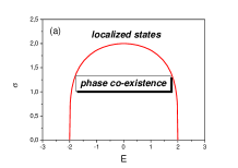
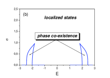
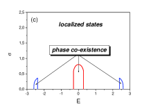
Figure 1: Phase diagram for $q=1$ (a), $q=2$ (b) and $q=3$ (c).

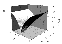
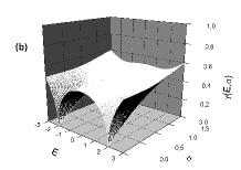
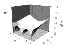
Figure 2: Surface plot $\gamma(E,\sigma)$ for $q=1$ (a), $q=2$ (b) and $q=3$ (c).

Therefore, in order to draw the phase diagram the analysis of the stable filter $H_{-}(w)$, Fig.1, is sufficient. The (unlimited) existence region of the localized states overlaps with that for the delocalized states (limited in both energy and disorder parameter). A number of such region corresponds to a number $q$ of the Landau subbands, see Fig.1. Each region is located near a center of old Landau subbands which existed without disorder.

As a result, the phase diagram contains one-phase regions (only localized states) and two-phase co-existence regions. The delocalized state phase is defined by zero Lyapunov exponent which needs no graphical illustrations. On the contrary, the localized state phase is characterized by the function $\gamma(E,\sigma)$ shown in Fig.2 in form of the surface plot. Note also that the results in Fig.1 and Fig.2 correspond to the thermodynamic limit.

The generally-accepted point of view [25] is that in the presence of a strong perpendicular magnetic field the extended states appear in the centers of disordered-broadened Landau bands and give rise to the integer quantum Hall effect. Instead, we obtained a more complex situation. In each Landau subband there is a region of phase co-existence. This region contains the critical points ($E=E_{c},\sigma=0$) where the localization length is divergent. Moreover, the observed anomalies (the canyon bottom in the surface plot of $\gamma(E,\sigma)$ in Fig.2) also lie in the region of phase co-existence.

Since the traditional viewpoint is based mostly on the results of numerical investigations, it is unclear how justified is here the thermodynamic limit transformation. It was reasonably noted [25] that we have to keep in mind that numerical calculations always deal with finite systems, while, strictly speaking, phase transitions exist only in infinite systems. It was also believed there that finite-size scaling theory could serve as theoretical framework to analyze data for finite systems, in order to extrapolate results to infinite system size. Our analysis of the phase diagram allows to understand better this conflicting situation.

First of all, the general result should be mentioned. Both Fig.1 and Fig.2 show that despite a quantitative difference, as a number of the Landau subbands $q$ increases, the same qualitative picture remains as it is observed for $q=1$. There is the co-existence region in each subband including the critical point $E_{c}$ and the relevant anomaly in the Lyapunov exponent (localization length). However, as $q$ increases, the region size systematically decreases. One can expect that in systems with large $q$ the two-phase region practically disappears. This is why there is some reasoning behind the statement [12] that the model (1) does not exhibit a metal-insulator transition. This is true indeed but only for a large number of Landau subbands.

The case of $q=1$ considered above allows us to establish also a link between systems with and without external magnetic field. As was noted, under a strong magnetic field but for $p=q=1$, Eq.(1) coincides formally with that without magnetic field. Therefore Fig.1a and Fig.2a illustrate also the phase diagram and the $\gamma(E,\sigma)$-surface plot without magnetic field. In other words, our correction of the statement [12, 25] that in the presence of a strong magnetic field extended states appear in the centers of Landau subbands, namely, a demonstration that the extended states could arise in fact in a wider region of the phase-coexistence, sheds also light on theoretical interpretation of the delocalized state existence without the magnetic field. Our important conclusion is that an emergence of the critical points is not a new effect caused by the magnetic field but the fundamental feature of a system even without the imposed field.

In the main region denoted in Fig.1 as the “localized states” the situation is simple and clear: a single phase exists for a given $E$ and $\sigma$ parameters. Since the analytical results correspond to the average over the random potential realizations, the existence of the delocalized states is here impossible. The random potential realizations could give slightly different results but this means, however, nothing but homophase fluctuations. All quantities are well defined and the terminology of the self-averaging quantities is justified here. This region of the phase diagram is not problematic also for standard numerical investigations. Indeed, the numerical study deals with the fluctuations in a homophase finite-size system, with the main focus on extrapolation of these results with typically bad statistics to the thermodynamic limit. Despite the fact that finite-size scaling is not strictly justified, this faces no fundamental objections. The problem is that the finite-size scaling works well in the cases when the region of the phase diagram under study contains points with a divergent correlation length. These points correspond to the relation $\gamma(E_{c},\sigma=0)=0$. However, as follows from Fig.2, such points are absent in the homophase region. The more so, the values of $\gamma(E,\sigma)$ are not small since they lie outside the canyon bottom.

When considering the phase co-existence region in the phase diagram, theory of the first-order phase transition is commonly used. It is obvious that use of the two parameters, $E$ and $\sigma$, does not define uniquely the phase state of a system: an ensemble of random potential $\varepsilon_{l,m}$ fluctuations could be heterophase, not homophase ones. A study of such ensembles faces a serious theoretical problem. It is common in experimental studies to characterize a large sample in terms of a single phase, giving no statistical analysis. However, in theoretical studies the macroscopic features are associated with the ensemble average. It is obvious that the averaging over the heterophase ensemble has no physical sense: this is true only for characteristics of individual homogeneous phases, self-averaging quantities lose here any sense [1].

The standard idea that an increase of the sample length $L$ brings us to the situation where the self-averaging effect automatically takes care of the ensemble statistical fluctuations and the statistical error can be estimated from sampling different realizations of the disorder [25] does not work here. An additional problem is that our approach [1, 2, 3] suggest no method to estimate the weight (probability) of individual phases.

Therefore, the phase co-existence region contains the critical points $(E=E_{c},\sigma=0$) where the localization length is divergent. However, the finite-size scaling cannot be used here, since the situation differs qualitatively from that for the second-order phase transition. That is, observation of the critical points does not necessarily justify use of the finite-size scaling.

The very fact of the heterophase ensemble existence produces fundamental difficulties for numerical investigations. In finite systems the phase concept is not defined, thus this is impossible to separated statistical contributions of the two phases. Indeed, how could one distinguish large but rare homophase fluctuation on a given parameter in a finite (typical small) size and the heterogeneous fluctuation, especially when the statistics is quite poor (relatively small number of random potential realizations)? We are not able to suggest any new algorithm for analysis of the relevant numerical investigations, we can only discuss the consequences of the heterogeneous ensemble existence.

4.4 Homophase interpretation

The possibility of phase co-existence is neglected tradicionally in numerical investigations [12]. It is believed that even if the phase diagram consists of the two regions with two phases, in each of these regions the relation between parameters $E$, $\sigma$ and the phase is unique. In other words, an existence of only homophase ensembles is assumed, which could arise in the case of the second-order phase transitions as well as without transitions. Let us discuss what could be a result of the substitution of a heterophase ensemble for homophase one, while performing numerical investigations. We will demonstrate that the general statement [25] follows uniquely from the homophase interpretation.

1) In the phase co-existence region both realizations with delocalized state, $\gamma\approx 0$, and localized state, $\gamma>0$, exist. As was said above these contributions cannot be separated (definition of a phase exists only for infinite systems [25]), and the statistical analysis leads to a formally calculated average $\langle\gamma\rangle>0$. This is equivalent to the statement that the system does not exhibit a metal-insulator transition (formally $\langle\gamma\rangle>0$ means existence of the localized states only). Therefore the homophase interpretation of 2-D numerical investigations with and without magnetic field leads to well-known conclusions [12, 25]

2) At the same time, the heterophase fluctuations should manifest themselves in the statistics as abnormally strong fluctuations of the $\gamma$ parameter, which is unusual for homophase systems and bring into question the treatment of the $\gamma$ parameter as the self-averaging quantity. The situation is complicated by the presence in the same region of the critical points ($E=E_{c},\sigma=0$) where the localization length diverges. Since such critical points arise typically in the second-order transitions, the quick conclusion suggests this interpretation with strong homophase fluctuations nearly the critical points instead of the real heterophase fluctuations. Moreveor, the observation of critical points could be also used to justify the finite-size scaling.

3) The anomaly of the Lyapunov exponent $\gamma(E,\sigma)$ near the critical points is well pronounced in Fig.2. This specific anomaly determined by the numerical methods, with a well pronounced peculiarity of the canyon bottom in the plot $\gamma(E,\sigma)$ permits a traditional interpretation [25] about critical points and the delocalized states.

The analysis above clearly demonstrates that the thermodynamic limit has no correct solution by means of numerical investigation. The extrapolation in terms of the finite-size scaling assumes an existence of the homophase ensemble. However, there is no proof of the the existence of such an ensemble within the same method. The heterophase idea is not constructive since it suggests no alternative to the finite-size scaling. The importance of exact analytical solutions in such conflicting situations is self-evident.

5 Conclusion

We have shown that the contradiction between the results of the present analytical approach (see also previous papers [1, 2, 3, 4, 5]) with those of numerical investigations [12, 25] arises due to different interpretations of the phase diagram. Our result [1, 2, 3] correspond to the thermodynamic limit where the phase concept is well defined [20]. It was also shown that the Anderson localization problem is characterized by the phase diagram with specific phase co-existence regions which need analysis in terms of first-order transitions. In those regions where the ensemble of heterophase fluctuations occurs the idea of self-averaging quantities fails. Analysis in the phase co-existence region is impossible for the finite systems since the phase concept is not defined here. Therefore, our analytical results [1, 2, 3, 4, 5] cannot be reproduced by means of numerical investigations since we cannot suggest any new algorithms for the numerical result analysis.

In its turn, the main numerical investigation results [12, 25] were obtained namely for the finite-size systems. Transition to the thermodynamic limit is traditionally performed in numerical investigations by means of the finite-size scaling. The latter assumes (directly and indirectly) existence of the ensemble of homophase fluctuations which permits result extrapolation to the infinite single-phase system. This approach fails in the case of two phase co-existence. Namely a wrong use of the hypothesis of a single phase in the heterophase case leads to incorrect theoretical conclusion about phase-transition absence in 2-D systems which obviously contradicts experimental data [10, 11]. Simultaneously, even in the framework of incorrect homophase interpretation numerical methods are able to detect phase co-existence regions, interpreting these as the critical points with relevant delocalized states.

References

- [1] V.N. Kuzovkov, W. von Niessen, V. Kashcheyevs and O. Hein, J. Phys.: Condens. Matter, 14, 13777 (2002).
- [2] V.N. Kuzovkov and W. von Niessen, Eur. Phys. J. B, 42, 529 (2004).
- [3] V.N. Kuzovkov and W. von Niessen, Physica A, 369, 251 (2006).
- [4] V.N. Kuzovkov and W. von Niessen, Physica A, 377, 115 (2007).
- [5] V.N. Kuzovkov, V Kashcheyevs, and W. von Niessen, J. Phys.: Condens. Matter, 16, 1683 (2004).
- [6] P.W. Anderson, Phys. Rev. 109, 1492 (1958).
- [7] P. Markoš, L.Schweitzer and M.Weyrauch, J. Phys.: Condens. Matter, 16, 1679 (2004).
- [8] I.M. Suslov, JETP, 101, 661 (2005). (cond-mat /0504557)
- [9] I.M. Suslov, cond-mat /0611504.
- [10] E. Abrahams, S.V. Kravchenko, M.P. Sarachik, Rev. Mod. Phys., 73, 251 (2001).
- [11] S.V. Kravchenko and M.P. Sarachik, Rept. Prog. Phys., 67, 1 (2004).
- [12] P. Marko, Acta physica slovaca,56, 561 (2006). (cond-mat /0609580)
- [13] E. Abrahams, P.W. Anderson, D.C. Licciardello, and T.V. Ramakrishnan, Phys. Rev. Lett. 42, 673 (1979).
- [14] I.M. Suslov, cond-mat /0610744.
- [15] J. W. Kantelhardt and A. Bunde, Phys. Rev. B 66, 035118 (2002).
- [16] S. L. A. de Queiroz, Phys. Rev. B 66, 195113 (2002).
- [17] Mp.P. Nightingale, Physica A,83, 561 (1976).
- [18] B. Derrida and J. Vannimenus, J.Phys.Lett., 41, L473 (1980).
- [19] J.-L, Pichard and G. Sarma, J.Phys. C, 14, L127 (1981).
- [20] R.J.Baxter, Exactly Solved Models in Statistical Mechanics (Academic Press, London, New York, 1982).
- [21] S. Ilani, A. Yacoby, D. Mahalu and H. Shtrikman, Science 292, 1354 (2001).
- [22] A.A. Shashkin, V.T. Dollgopolov, G.V. Kravchenko, M. Wendel, R. Schuster, J.P. Kotthaus, P.J. Haug, K. von Klitzing, K. Ploog, N. Nickel, and W. Schlapp, Phys. Rev. Lett. 73, 3141 (1994).
- [23] Y. Meir, Phys. Rev. B 61, 16470 (2000).
- [24] B. Spivak, Phys. Rev. B 67, 125205 (2003).
- [25] B. von Huckestein, Rev. Mod. Phys. 67, 357 (1995).
- [26] X.R. Wang, C.Y. Wong, and X.C. Xie, Phys.Rev.B, 59, R5277 (1999).
- [27] T.F. Weiss. Signals and systems. Lecture notes. http:// umech.mit.edu/ weiss/ lectures.html