XMM-Newton studies of a massive cluster of galaxies:
RXCJ2228.6+2036

We present the X-ray properties of a massive cluster of galaxies (RXCJ2228.6+2036 at $z=0.421$) using XMM-Newton data. The X-ray mass modeling is based on the temperature and density distributions of the intracluster medium derived using a deprojection method. We found that RXCJ2228.6+2036 is a hot cluster ($T_{500}=8.92^{+1.78}_{-1.32}$ keV) showing a cooling flow rate of $12.0^{+56.0}_{-12.0}$ M_⊙yr^-1 based on spectral fitting within the cooling flow radius ($r_{cool}=147\pm 10$ kpc). The total cluster mass is $M_{500}=(1.19\pm 0.35)\times 10^{15}$ M_⊙ and the mean gas mass fraction is $f_{gas}=0.165\pm 0.045$ at $r_{500}=1.61\pm 0.16$ Mpc. We discussed the PSF-correction effect on the spectral analysis and found that for the annular width we chose the PSF-corrected temperatures are consistent with those without PSF-correction. We observed a remarkable agreement between X-ray and SZ results, which is of prime importance for the future SZ survey. RXCJ2228.6+2036 obeys the empirical scaling relations found in general massive galaxy clusters (e.g. $S$–$T$, $M$–$T$, $L$–$T$ and $M$–$Y$) after accounting for self-similar evolution.

1 Introduction

The gravitational growth of fluctuations in the matter density distribution can be traced by the evolution of the galaxy cluster mass function (e.g. Schuecker et al. 2003). The hot and distant clusters are at the upper end of the mass distribution, thus they can be used to probe the cosmic evolution of large-scale structure and are therefore fundamental probes for cosmology. But to date still very few hot and distant clusters are known. Therefore, it is important to study such clusters in detail, especially in X-ray.

RXCJ2228.6+2036 is one of the distant (z = 0.421) and X-ray luminous clusters of galaxies in the northern sky. It is suspected to be massive and hot, and was well recognized as an extended X-ray source in the ROSAT All-Sky Survey, included in both the NORAS galaxy cluster survey (Böhringer et al. 2000) and the ROSAT Brightest Cluster Sample (Ebeling et al. 2000).

The first combined SZ versus X-ray analysis for RXCJ2228.5+2036 is based on the SZ data from the Nobeyama Radio Observatory (NRO) 45 m radio telescope and the X-ray data from ROSAT/HRI. It shows that RXCJ2228.6+2036 is a hot and massive cluster with $T=10.4\pm 1.8$ keV, $M_{tot}(r<R_{v}=r_{178}=2.9$ Mpc) = $(1.8\pm 0.4)\times 10^{15}$ M_⊙, and with a gas mass fraction of $f_{gas}=0.22\pm 0.06$ (Pointecouteau et al. 2002). Recently, LaRoque et al. (2006) performed the Chandra X-ray versus OVRO/BIMA interferometric SZ effect measurements for the same cluster, giving $T=8.43^{+0.78}_{-0.71}$ keV, $f_{gas}=0.138\pm 0.009$ from the X-ray data, and $f_{gas}=0.188^{+0.035}_{-0.031}$ from the SZ data at $r_{2500}$. RXCJ2228.6+2036, as one of the clusters in the sample of X-ray luminous galaxy clusters with both X-ray (Chandra) and SZ observations in Morandi et al. (2007), has a temperature of $T=6.86^{+0.89}_{-0.71}$ keV and a total mass of $M_{tot}=(4.90\pm 4.35)\times 10^{14}$ M_⊙ at $r_{500}=1033\pm 464$ kpc. However, the above results are all based on the mass modeling under the assumption of isothermality of the ICM. The XMM-Newton EPIC instruments have both high spatial and spectral resolutions and a large field of view, and are therefore suitable for a spatially resolved spectral analysis. We make use of XMM-Newton observations to carry on a detailed study of RXCJ2228.6+2036 based on the X-ray mass modeling using a spatially resolved radial temperature distribution and perform a detailed X-ray versus SZ comparison.

The structure of this paper is as follows: Sect. 2 describes the data, background subtraction method and spectral deprojection technique. Sect. 3 presents the spectral measurements using different models to derive the radial temperature profile, cooling time and mass deposition rate. In Sect. 4 we show the radial electron density profile and X-ray mass modeling. In Sect. 5 we discuss the impact of the PSF correction on the spectral analysis, and compare RXCJ2228.6+2036 to the SZ measurements and the empirical scaling relations for massive galaxy clusters. We draw our conclusion in Sect. 6.

Throughout this paper, unless explicitly stated otherwise, we use the 0.5-10 keV energy band in our spectral analysis. The cosmological model used is $H_{0}$ = $70$ km s^-1Mpc^-1, $\Omega_{m}$ = 0.3, and $\Omega_{\Lambda}$ = 0.7, in which 1^′ corresponds to 332.7 kpc at the distance of RXCJ2228.6+2036.

2 Observation and data reduction

2.1 Data preparation

RXCJ2228.6+2036 has been observed for 26 ksec in November 2003 by XMM-Newton and its observation ID is 0147890101. For our purpose, we only use EPIC data (MOS1, MOS2 and pn). The observations are performed with a thin filter and in the extended full frame mode for pn and the full frame mode for MOS. Throughout this analysis, we only use the events with FLAG=0, and with PATTERN$\leq$4 for pn and PATTERN$\leq$12 for MOS. The reduction was performed in SAS 7.1.0.

The light curve of the observation shows some flares (i) in the hard band (above 10 keV for MOS and above 12 keV for pn), possibly caused by the particle background, and (ii) in the soft band (0.3-10 keV), possibly due to the episodes of ‘soft proton flares’ (De Luca & Molendi 2004). Therefore both the hard and the soft bands are used to select the good time intervals (GTI) as described in Zhang et al. (2006). The GTI screening procedure gives us 22 ks MOS1 data, 22 ks MOS2 data, and 18 ks pn data.

We applied the SAS task edetect chain to detect the point sources (the radius of the point sources is $0.6^{\prime}$ containing 93% flux from the point source), and excised all of them from the cluster region. Then, a SAS command evigweight was used to create the vignetting weighted column in the event list to account for the vignetting correction for the effective area.

Due to read-out time delay, the pn data require a correction for the Out-of-time (OOT) events. We created the simulated OOT event file and used it to account for this (see Strüder et al. 2001 ) in our analysis.

2.2 Background subtraction

The XMM-Newton background normally consists of the following two components. i) Particle background: high energy particles such as cosmic-rays pass through the satellite and deposit a fraction of their energy on the detector. It dominates at high energies and shows no vignetting. ii) Cosmic X-ray Background (CXB): the CXB varies across the sky (Snowden et al. 1997). It is more important at low energies and shows a vignetting effect.

We choose the blank sky accumulations in the Chandra Deep Field South (CDFS) as the background (Zhang et al. 2007), which was also observed with the thin filter. We applied the same reduction procedure to the CDFS as to the cluster in the same detector coordinates, and the effective exposure time we obtained for CDFS is 54 ks for pn, 61 ks for MOS1 and 61 ks for MOS2. RXCJ2228.6+2036 is a distant cluster ($z=0.421$), and we estimated that the signal-to-noise ratio of the region $6^{\prime}<R<6.5^{\prime}$ is about 20%, so we can approximately assume that the emission of the cluster only covers the inner part of the field of view ($R<6^{\prime}$). The outer region ($6.5^{\prime}<R<8^{\prime}$) can thus be used to monitor the residual background. Here we applied a double-background subtraction method to correct for these two kinds of background components as used in Arnaud et al. (2002). First we estimate the ratio of the particle background, $\alpha$, between RXCJ2228.6+2036 and CDFS from the total count rate in the high energy band (10-12 keV for MOS and 12-14 keV for pn), as described in Pointecouteau et al. (2004). $S_{0}$ and $B_{0}$ are the background spectra of the cluster and CDFS in the region of $6.5^{\prime}<r<8^{\prime}$ with an area of $A_{0}$, and $S_{i}$ and $B_{i}$ for spectra in the $i$th ring of the cluster and CDFS with an area of $A_{i}$. Then the cluster spectrum, after the double-background subtraction, $S(i)$ is (e.g. Jia et al. 2006, Zhang et al. 2006):

$$S(i)=S_{i}-\alpha B_{i}-\frac{A_{i}}{A_{0}}(S_{0}-\alpha B_{0})$$ (1)

2.3 Spectral deprojection

The combined image of MOS1 and MOS2 in the energy band 0.5-10 keV is shown in Fig. 1. It is corrected for vignetting and smoothed with a maximum Gaussian smoothing size of $\sigma=5$ pixels. As shown in this figure, the X-ray emission of RXCJ2228.6+2036 appears to be extended and almost symmetric except for some bright point sources (which were subtracted before the spectrum extraction, see Sect. 2.1). We extract the spectra from annular regions centered on the emission peak, and the width of each ring is determined according to the criterion described in Zhang et al. (2007): $\sim$2000 net counts per bin in 2-7 keV to get a temperature with $\sim$15% uncertainty. Considering the PSF (Point Spread Function) effect of XMM-Newton EPIC, whose Full Width at Half Maximum (FWHM) is $5^{\prime\prime}$ for MOS and 6$\arcsec$ for pn, the minimum width of each ring was set at $0.5^{\prime}$. We thus obtained 5 annuli to extract spectra out to $6^{\prime}$.

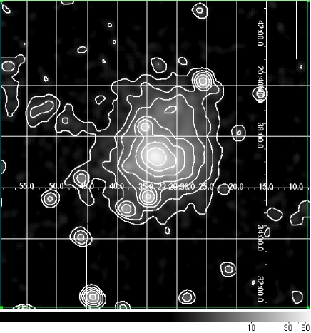
Figure 1: The combined image of MOS1 and MOS2 of RXCJ2228.6+2036 ($12^{\prime}\times 12^{\prime}$) corrected for vignetting and smoothed with a maximum Gaussian smoothing size of $\sigma=5$ pixels.

The deprojected spectra are calculated by subtracting all the contributions from the outer regions. Within each radial range, we assume the same spectrum per unit volume. The deprojected spectrum of the $i$th shell is then calculated by subtracting the contributions from the $i$+1th shell to the outmost one (e.g. Matsushita et al. 2002 and Nulsen & Böhringer 1995). The detailed calculation procedures are described as in Jia et al. (2004, 2006):

$$D(i)=\left[S(i)-\sum_{k=i+1}^{N}C_{v}(k,i)\cdot D(k)\right]/C_{v}(i,i),$$ (2)

here $D(i)$ is the deprojected spectrum of the $i$th shell, $S(i)$ is the double-background subtracted spectrum of the $i$th shell and $C_{v}(k,i)$ is the fraction of the volume of the $k$th shell projected to the $i$th ring.

The on-axis rmf (response matrix file) and arf (auxiliary responds file) are generated by the SAS task rmfgen and arfgen and are used to recover the correct spectral shape and normalization of the cluster emission components.

3 Spectral analysis

3.1 Radial deprojected temperature profile

The spectral analysis is carried out in XSPEC version 11.3.2 (Arnaud 1996). To study the temperature distribution of RXCJ2228.6+2036, we perform a joint fit to the spectra of pn and MOS with an absorbed Mekal model:

$$Model_{1}=Wabs(N_{H})\times Mekal(T,z,A,norm),$$ (3)

in which Wabs is a photoelectric absorption model (Morrison & McCammon 1983) and Mekal is a single-temperature plasma emission model (Mewe et al.1985, 1986; Kaastra 1992; Liedahl et al. 1995). The temperature $T$, metallicity $A$ and normalization (emission measure) $norm$ are free parameters. We fixed the redshift $z$ to 0.421 and the absorption $N_{H}$ to the Galactic value 4.68$\times$10²⁰ cm^-2 (Dickey & Lockman 1990). The fitting results are listed in Table 1 and the central spectra fitted by this model are shown as Fig. 3(a).

Table 1: The best-fit free parameters of RXCJ2228.6+2036 by the single-temperature model: the temperature $T$; the abundance $A$ and the normalized constant $norm$ for the simultaneously fitting of pn and MOS. $norm=10^{-14}/(4\pi(D_{A}\times(1+z))^{2})\int n_{e}n_{H}dV$, where $D_{A}$ is the angular size distance to the source (cm) and $n_{e}$ is the electron density (cm^-3). $L_{bol}$ represents the bolometric luminosity (0.01-60 keV) in the units of $10^{44}$ erg s^-1. The errors represent a confidence level of 90%.

$r$(′)	$T$ (keV)	$A$ (solar)	$norm$($10^{-3}$cm-5)	$\chi^{2}_{\mathrm{red}}$/$dof$	$L_{bol}$($10^{44}$ erg s-1)
0.0-0.5	$8.26^{+1.02}_{-0.92}$	$0.31^{+0.19}_{-0.18}$	$0.72\pm 0.03$	1.12/251	$4.65^{+0.38}_{-0.31}$
0.5-1.0	$11.65^{+2.54}_{-1.78}$	$0.20^{+0.27}_{-0.2}$	$0.88\pm 0.05$	1.02/262	$6.73^{+0.58}_{-0.76}$
1.0-1.75	$9.03^{+1.82}_{-1.27}$	$0.30^{+0.25}_{-0.24}$	$1.08\pm 0.06$	1.00/196	$7.33^{+0.72}_{-0.74}$
1.75-3.0	$8.21^{+1.66}_{-1.26}$	$0.12^{+0.25}_{-0.12}$	$1.28\pm 0.07$	0.86/189	$7.89^{+0.81}_{-1.01}$
3.0-6.0	$5.10^{+5.68}_{-2.22}$	0.12(fixed)	$0.73^{+0.13}_{-0.10}$	0.51/59	$3.34^{+1.20}_{-1.96}$

The deprojected temperature profile shows a drop in the core and a decrease in the outer regions (see the diamonds in the upper panel of Fig. 2), which can be fitted by the following formula (Xue et al. 2004):

$$T(r)=T_{0}+\frac{A}{r/r_{0}}exp(-\frac{(\ln r-\ln r_{0})^{2}}{\omega}).$$ (4)

The best fit parameters are: $A$ = $4.880\pm 0.001$ keV, $r_{0}=2.494\pm 0.003^{\prime}$, $\omega$ = $2.232\pm 0.004$, $T_{0}=3.084\pm 0.001$ keV, $\chi^{2}_{red}=0.31$, and the best-fit profile is shown as the solid line in the upper panel of Fig. 2. From the temperature distribution, we can estimate the normalization-weighted temperature within $6^{\prime}$, $t_{mean}=8.57^{+2.39}_{-1.56}$ keV, which is consistent with the results of Pointecouteau et al. (2002) and LaRoque et al. (2006) within the error bars and a little higher than that of Morandi et al. (2007). The diamonds in the bottom panel of Fig. 2 show the deprojected abundance distribution of RXCJ2228.6+2036.

Figure 2: Upper panel: Radial temperature profile of RXCJ 2228.6+2036. Diamonds: the deprojected temperature and the solid line is the best-fit profile. Stars: for the PSF-corrected temperature (see Sect. 5.1). We offset the stars $5^{\prime\prime}$ to the left so as to illustrate these two kinds of temperature clearly. Bottom panel: Radial deprojected abundance of RXCJ2228.6+2036. The confidence level is 90%.

3.2 Mass deposition rate

The temperature drop in the central part of RXCJ2228.6 +2036 might indicate the existence of a cooling flow in the center. We thus estimate the parameters of the cooling flow as follows.

The cooling time $t_{cool}$ is the time scale during which the hot gas loses all its thermal energy, which is calculated as (e.g. Chen et al. 2007):

$$t_{cool}=\frac{5}{2}\frac{n_{e}+n_{i}}{n_{e}}\frac{k_{B}T}{n_{H}\Lambda(T)}$$ (5)

where $\Lambda(T)$ is the cooling function of the gas, and $n_{e}$, $n_{i}$ and $n_{H}$ are the number densities of the electrons, ions and hydrogen, respectively. Here for the nearly fully ionized plasma in clusters, $n_{e}=1.2n_{H}$ and $n_{i}=1.1n_{H}$. The determination of $n_{e}$ is explained later in Sect. 4.1. The cooling time $t_{cool}$ of the inner two regions is given in Table 2. The cooling radius designates the region inside which the hot gas loses all its thermal energy within a cluster life time scale, usually using the age of the universe ($1.04\times 10^{10}$ yr at $z=0.421$). The resulting cooling radius for RXCJ2228.6+2036 is $r_{cool}=147\pm 10$ kpc.

Table 2: The cooling time and the cooling flow rate determined with the spatial method of the inner two regions of RXCJ2228.6+2036. The errors are at the 68% confidence level. $1^{\prime}=332.7$ kpc.

$r_{1}$	$r_{2}$	$t_{cool}$(yr)	$\dot{M}$(M⊙yr-1)
$0^{\prime}$	$0.5^{\prime}$	$1.18\pm 0.07\times 10^{10}$	$200.2\pm 12.4$
$0.5^{\prime}$	$1^{\prime}$	$3.58\pm 0.27\times 10^{10}$	$414.7\pm 32.6$

We also fit the central spectra of pn and MOS by adding a standard cooling flow model to the isothermal Mekal component:

$$Model_{2} = Wabs(N_{H})\times(Mekal(T,z,A,norm)+$$ (6)

$$Zwabs(\Delta N_{H})\times Mkcflow(\dot{M})).$$

Wabs and Mekal have been described in Sect. 3.1, Zwabs is an intrinsic photoelectric absorption model (Morrison & McCammon 1983), and Mkcflow is a cooling flow model (Fabian, 1988); $\Delta N_{H}$ is the intrinsic absorption and $\dot{M}$ is the rate of gas cooling out of the flow. The fitting results show that the mass deposition rate in the central region $r<0.5^{\prime}$ is $14.0^{+64.0}_{-14.0}$ M_⊙yr^-1 (see Table 3), so within $r_{cool}$ $\dot{M}=12_{-12}^{+56}$ M_⊙yr^-1. Fig. 3(b) presents the central spectra fitted by this model.

Table 3: The best-fit parameters for the central region of RXCJ2228.6+2036 by $Model_{2}$. The $lowT$ is fixed on 0.01 keV and $1^{\prime}=332.7$ kpc. The errors are at the 90% confidence level.

r	$T_{mekal}$	low$T_{cf}$	high$T_{cf}$	A	norm	$\dot{M}$	$\Delta n_{H}$	$\chi^{2}_{\mathrm{red}}$/$dof$
	(keV)	(keV)	(keV)	(solar)	($10^{-3}$cm-5)	(M⊙)	($10^{22}$cm-2)
$0^{\prime}-0.5^{\prime}$	$8.54^{+2.27}_{-1.18}$	0.01 (fix)	=$T_{mekal}$	$0.32\pm 0.19$	$0.70^{+0.05}_{-0.12}$	$14.0^{+64.0}_{-14.0}$	0.0(fix)	1.12/250

Figure 3: The spectra of the central region (r $<0.5^{\prime}$) for joint fit of pn (bold crosses) and MOS (faint crosses) of RXCJ2228.6+2036. a) fitted by a single-temperature model; b) fitted by a cooling flow model with an isothermal Mekal component. In b) we plot the isothermal and the cooling flow components respectively, and the lower lines below the crosses represent the multiphase components of pn (bold line) and MOS (faint lines), which show that the multiphase components only contribute a little to the emissions.

4 Mass determination

4.1 Electron density

We divided the $r<6^{\prime}$ region into 13 annuli centered on the emission peak, where the width of each annular region is determined to obtain at least 2000 total counts in each annulus region in 0.5-10 keV. After the vignetting correction and the double-background subtraction, the surface brightness profile for RXCJ2228.6+2036, $S(r)$, is derived, which can be fitted by a double-$\beta$ model (as Eq. 9) convolved with the PSF matrices (Ghizzardi 2001) to correct for the PSF effect. Using the deprojection technique described in Sect. 2.3, we deproject the double-$\beta$ model (PSF corrected) and obtain the count rate of each corresponding shell, $Ctr(i)$. Since the temperature and abundance profiles are known, giving $T(i)$, $A(i)$ and $Ctr(i)$ in the $i$th shell, we can derive the corresponding $norm(i)$ in XSPEC with $Model_{1}$. The radial electron density $n_{e}$ of each region can be determined from Eq. (8), shown as stars in Fig. 4.

$$norm(i)=10^{-14}/(4\pi D^{2})\cdot\int n_{e}n_{H}dV.$$ (7)

We fit the derived electron density (the stars in Fig. 4) with the double-$\beta$ model (Chen et al. 2003):

$$n_{e}(r)=n_{01}{\left(1+{(\frac{r}{r_{c1}})}^{2}\right)}^{-{\frac{3}{2}}\beta_{1}}+n_{02}{\left(1+{(\frac{r}{r_{c2}})}^{2}\right)}^{-{\frac{3}{2}}\beta_{2}},$$ (8)

the best-fit parameters are: $n_{01}$ = $0.0027\pm 0.0002$ cm^-3, $r_{c1}$ = $2.5480\pm 0.0002$ arcmin, $\beta_{1}$ = $1.4031\pm 0.0001$, $n_{02}$ = $0.0109\pm 0.0001$ cm^-3, $r_{c2}$ = $0.6547\pm 0.0004$ arcmin, $\beta_{2}$ = $1.5474\pm 0.0001$, $\chi^{2}_{red}=0.71$, $dof$=7. And the best-fit profile is shown as the solid line in Fig. 4.

Figure 4: The deprojected electron density profile of RXCJ2228.6+2036 after PSF correction. The error bars are at the 68% confidence level. The solid line is the best-fit profile from a double-$\beta$ model fitting.

4.2 Total mass

Once we have derived the radial temperature profile $T(r)$ and electron density profile $n_{e}(r)$ for RXCJ2228.6+2036, the integrated total mass of this cluster at radius $r$ can be calculated under the assumptions of hydrostatic equilibrium and spherical symmetry by the following equation (Fabricant et al. 1980):

$$M_{tot}(<r)=-\frac{k_{B}Tr^{2}}{G\mu m_{p}}\left[\frac{d(\ln{n_{e}})}{dr}+\frac{d(\ln{T})}{dr}\right],$$ (9)

here $k_{B}$ is the Boltzmann constant, $G$ is the gravitational constant and $\mu$ is the mean molecular weight in units of the proton mass $m_{p}$ (we assume $\mu=0.6$ in this work). The mass uncertainties are obtained from the uncertainties of the temperature and the electron density calculated by Monte-Carlo simulations. We obtained 250 redistributions of the parameterized temperature and electron density profiles by fitting to the data points varied within the Gaussian error bars of the measurements. The uncertainties of all the other properties of RXCJ2228.6+2036 are also calculated from the 250 simulated clusters.

Then, we derived the total mass profile of RXCJ2228.6 +2036, shown in Fig. 5, and $M_{tot}=(1.36\pm 0.51)\times 10^{15}$ M_⊙ at $6^{\prime}$ at the 68% confidence level.

Figure 5: The total mass profile of RXCJ2228.6+2036, and the error bars (dotted lines) are at the 68% confidence level. The vertical line indicates $r_{500}=1.61\pm 0.16$ Mpc.

A physically meaningful radius for the mass measurement is defined as $r_{500}$, the radius within which the mean gravitational mass density $<\rho_{tot}>=500\rho_{c}$, where $\rho_{c}=3H^{2}/(8\pi G)$ is the critical cosmic matter density. For our calculations, we use the value of $\rho_{c}$ at the cluster redshift, i.e., $\rho_{c}=9.2\times 10^{-30}$ g cm^-3. This radius is still well covered by the observations. From the mass profile we derive $r_{500}=1.61\pm 0.16$ Mpc for RXCJ2228.6+2036, corresponds to $4.8^{\prime}\pm 0.5^{\prime}$, and the total mass within it is about $M_{500}=(1.19\pm 0.35)\times 10^{15}$ M_⊙. The mass derived from Chandra data by Morandi et al. (2007) is $M_{tot}=(4.90\pm 4.35)\times 10^{14}$ M_⊙ within $r_{500}=1033\pm 464$ kpc, still consistent with ours within the error bars. In our analysis, the extrapolated value of $r_{vir}=2.48\pm 0.38$ Mpc $=7.5^{\prime}\pm 1.1^{\prime}$ and $M_{vir}=(1.55\pm 0.72)\times 10^{15}$ M_⊙, which agrees with what Pointecouteau et al. (2002) derived.

4.3 gas mass and gas mass fraction

In galaxy clusters, gas is an important component involving complex physics. From the electron density we calculate the gas mass and the gas mass fraction defined as $f_{gas}(r)=M_{gas}(r)/M_{tot}(r)$. Fig. 6 shows the gas mass fraction profile of RXCJ2228.6+2036. The gas mass fraction at $6^{\prime}$ is $f_{gas}=0.17\pm 0.06$, consistent within the error bars with the results of LaRoque et al. (2006) from the Chandra X-ray and OVRO/BIMA interferometric SZ effect measurements: $f_{gas}=0.138\pm 0.009$ from the X-ray data and $f_{gas}=0.188^{+0.035}_{-0.031}$ from the SZ data. It also agrees with the WMAP measured baryon fraction of the Universe $f_{b}=\Omega_{b}/\Omega_{m}=0.166$ (Spergel et al. 2003).

Figure 6: The gas mass fraction profile of RXCJ2228.6+2036. The dashed horizontal line indicates the WMAP measurement of $f_{b}=\Omega_{b}/\Omega_{m}=0.166$ (Spergel et al. 2003) and the vertical line indicates $r_{500}=1.61\pm 0.16$ Mpc. The error bars (dotted lines) are at the 68% confidence level.

5 Discussion

5.1 PSF-corrected spectra

The spatially resolved spectral analysis is affected by the PSF. To correct for the PSF effect, we first calculate the redistribution matrix, $F_{ij}$, which is the fractional contribution in the $i$th ring coming from the $j$th ring (Pratt & Arnaud 2002). We get this redistribution from our best fitted double-$\beta$ model of electron density (converted to emission measure profile) and the PSF matrices (Ghizzardi 2001). Since we have divided our cluster into 5 regions, we can obtain the fractional contribution in each ring coming from all the bins, and in Fig. 7, we plot the contribution from the bin, all inner and outer bins.

Figure 7: Redistributions due to the XMM-Newton PSF: the diamonds represent the contribution coming from the bin, the stars from the inner bins and the triangles from the outer bins.

Here, $O_{i}$ is the observed spectrum of the $i$th ring after a double-background subtraction, $S_{i}$ is the spectrum without PSF effect, so for our cluster RXCJ2228.6+2036, we have:

$$\left(\begin{array}[]{ccccc}F_{11}&F_{12}&F_{13}&F_{14}&F_{15}\\ F_{21}&F_{22}&F_{23}&F_{24}&F_{25}\\ F_{31}&F_{32}&F_{33}&F_{34}&F_{35}\\ F_{41}&F_{42}&F_{43}&F_{44}&F_{45}\\ F_{51}&F_{52}&F_{53}&F_{54}&F_{55}\end{array}\right)\cdot\left(\begin{array}[]{c}S_{1}\\ S_{2}\\ S_{3}\\ S_{4}\\ S_{5}\end{array}\right)=\left(\begin{array}[]{c}O_{1}\\ O_{2}\\ O_{3}\\ O_{4}\\ O_{5}\end{array}\right).$$ (25)

From this function we can derive $S_{i}$, which indicates the spectra after the PSF correction. Then, we deproject these spectra $S_{i}$ by the deprojection technique described in Sect. 2.3, and thus derive the PSF corrected deprojected spectra. Fitting these spectra with $Model_{1}$, we obtained the PSF-corrected deprojected temperatures, shown as stars in the upper panel of Fig. 2.

We find that the PSF-corrected temperatures agree with the measurements without PSF-correction. This may be due to the broad width of the regions we chose. However it should be noted here that these spectral fits are not as good as those in Sect. 3.1 because the PSF-correction procedure introduces significant uncertainties, mainly due to the inversion process (see Eq. 11).

5.2 Gas pressure and comparison with the SZ data

With the temperature profile $T(r)$ and electron density profile $n_{e}(r)$, we can derive the gas pressure profile of RXCJ2228.6+2036 as:

$$P(r)=n_{e}(r)k_{B}T(r).$$ (26)

In terms of observables, the gas pressure can be checked against the SZ effect (Sunyaev & Zel’dovich 1972) coming from the cluster. Indeed the SZ effect is directly proportional to the integrated pressure over the line of sight:

$$S_{SZ}(r) = \frac{\sigma_{T}}{m_{e}c^{2}}\int{k_{B}T(r)n_{e}(r)dr}\cdot f_{SZ}(v,T)$$ (27)

$$= \frac{\sigma_{T}}{m_{e}c^{2}}\int{P(r)dr}\cdot f_{SZ}(v,T),$$

where $k_{B}$, $m_{e}$, $c$ and $\sigma_{T}$ are the Boltzmann constant, the electron mass, the speed of light and the Thomson cross-section; $f_{SZ(v,T)}$ represents the SZ spectral shape (including the relativistic corrections as computed by Pointecouteau et al. 1998).

Here we integrated the gas pressure of RXCJ2228.6 +2036 using Eq. (13), convolved with the PSF of the 45 m radio telescope NRO (the beam size at 21 GHz: $\theta_{FWHM}\sim 80$ arcsec) and then compared it with the SZ radial profile (Pointecouteau et al. 2002) in Fig. 8. The diamonds are from the SZ data and the solid line represents our result. We found a remarkable agreement within the error bars.

Figure 8: The integrated X-ray pressure profile of RXCJ2228.6 +2036 convolved with the PSF of the SZ telescope (the solid line) and compared with the SZ radial profile (the diamonds) derived by Pointecouteau et al. (2002). All the errors are at the 68% confidence level.

The good agreement of the X-ray and SZ surface brightness profile in Fig. 8 may lend itself to test biases in the derivation of the pressure profile from the X-ray data. The most interesting aspects concern a bias in the temperature measurement in the presence of a multitemperature ICM (e.g. Mazzotta et al. 2004, Vikhlinin 2006) and the overestimate of the gas density due to the enhancement of the surface brightness if the gas is clumpy. In the following we will investigate how these two effects are modifying the comparison of the X-ray and SZ data.

If we assume that the ICM is in rough pressure equilibrium the two bias effects on the temperature and the density are actually linked (for $n_{e}\cdot T=$ constant). While local unresolved density inhomogeneities will lead to an overestimation of the density and the prediction of a too high SZ-signal, the temperature of a clumpy medium will be underestimated compared to a mass average and result in an underprediction of the SZ signal. So both effects are at least partly compensating each other in our study.

Quantitatively the overestimation of the gas density is given by:

$$C^{\prime}=\frac{<n_{e}^{2}>}{<n_{e}>^{2}},$$ (28)

where the overestimation factor is $C=\sqrt{C^{\prime}}$. To quantify the underestimation of the temperature for this hot cluster, we can approximately use the approach of Mazzotta et al. (2004) (Eq.14) which yields:

$$\frac{T_{sl}}{T}=R=\frac{<n_{e}><n_{e}^{1.75}>}{<n_{e}^{2.75}>},$$ (29)

where $T_{sl}$ is a good approximation of the spectroscopic temperature as would be obtained from data analysis of Chandra and XMM-Newton observations for a multi-temperature plasma, and $T$ the mass weighted mean.

As an example we calculate these effects for a homogeneous distribution with a lower and higher cutoff of, $T_{1}=<T>-\varepsilon$ and $T_{2}=<T>+\varepsilon$, respectively. A more general distribution can also be seen as a superposition of many of these ‘top-hat’ distributions. Fig. 9 shows the enhancement factors $C$ and $R$ as a function of the distribution width parameter, $\varepsilon$. We note that the two effects don’t cancel each other, but the effect of the temperature underestimate is about 2-3 times larger than the overestimat-e due to clumpiness. Still the overall effect is not dramatic and does therefore not provide a very good diagnostics. Even for a broad temperature distribution with $\varepsilon/<T>\approx 0.75$ for example, covering a temperature range (from the lower temperature to the higher temperature) of a factor of 7, we obtain an SZE underestimate of about 30% and a gas mass overestimate of about 18%.

Figure 9: Overestimation factor of the gas density $C$ and underestimation of the spectroscopic like temperature versus the mass weighted temperature $R$ as a function of the width of a homogeneous temperature distribution in the presence of pressure equilibrium. The combined effect $C\times R$ is for the underestimation of SZE. For the definition of the parameters see the text.

This has also implications on the mass measurement. While the pressure profile and its derivative can be directly taken from the SZ-profile, we still require an independent absolute temperature measurement for the normalization of the mass profile. The above calculation shows now, that we don’t obtain very precise new information on a possibly low biased temperature due to a multiphase ICM from having simultaneous X-ray and SZ observations. In the above example a temperature and mass underestimation of 40% is only indicated by an SZ deviation of 30%.

5.3 Gas entropy and the $S-T$ relation

Following Ponman et al. (1999), we defined the entropy of the gas in clusters as:

$$S(r)=\frac{T(r)}{n_{e}(r)^{\frac{2}{3}}}.$$ (30)

This entropy corresponds to the heat supplied per particle for a given reference density. Fig. 10 shows the entropy distribution as a function of radius, where the diamonds represent the entropy obtained from the spectra fitting results and the solid line from the best fitted $T(r)$ and $n_{e}(r)$ profiles.

Figure 10: The entropy distribution of RXCJ2228.6+2036. The diamonds represent the entropy derived from the spectral fitting results and the solid line from the best fitted $T(r)$ and $n_{e}(r)$ profiles. The vertical line shows $r_{500}=1.61\pm 0.16$ Mpc. The error bars are at the 68% confidence level.

Pratt et al. (2006) have shown for the $S-T$ relation measured from a sample of 10 local and relaxed clusters observed by XMM-Newton, that $S_{0.3}\propto T_{X}^{0.64}$, where $S_{0.3}$ means the entropy at $0.3r_{200}$ and $T_{X}$ is the mean temperature in the region of $0.1r_{200}<r<0.5r_{200}$. For RXCJ2228.6+2036, $S_{0.3r200}=959\pm 130$ keV cm² and $T_{X}=8.91^{+1.91}_{-1.33}$ keV. The $S_{0.3r200}$ versus $T_{X}$ for RXCJ2228.6+2036 is plotted on the $S-T$ relation derived by Pratt et al. (2006), shown in Fig. 11. The diamonds and the best fit line (the solid line) are from Pratt et al. (2006), and the star indicates the result of RXCJ2228.6+2036. It shows that our entropy value for RXCJ2228.6+2036 is consistent (within the 1$\sigma$ error bars) with Pratt et al. (2006) $S-T$ relation at 0.3$r_{200}$, once corrected for the expected evolution in a self-similar scenario of structure formation.

Figure 11: Comparison of the present result with the $S-T$ relation of Pratt et al. (2006). The star indicates the result of RXCJ2228.6+2036, and the diamonds and the best-fitted $S-T$ relation line (the solid line) come from Pratt et al. (2006). Here $h(z)=[0.3(1+z)^{3}+0.7]^{\frac{1}{2}}$. The error bars of the star are at the 68% confidence level.

5.4 $M-T$ and $L-T$ relations

From the above analysis, we derived the temperature, mass and X-ray luminosity (see Table 1) of RXCJ2228.6+2036: within $r_{500}=4.8^{\prime}$, $M_{500}=(1.19\pm 0.35)\times 10^{15}$ M_⊙, $T_{500}=8.92^{+1.78}_{-1.32}$ keV and $L_{bol,500}=28.83^{+3.69}_{-4.78}\times 10^{44}$ erg s^-1. Therefore we can compare RXCJ2228.6+2036 to the empirical scaling relations for massive galaxy clusters, e.g. $M_{500}-T_{500}$ and $L_{bol,500}-T_{500}$ derived from XMM-Newton data, such as in Kotov & Vikhlinin (2005) based on 10 clusters at $z=0.4-0.7$, Arnaud et al. (2005) based on 10 nearby clusters ($z<0.15$) and Zhang et al. (2008) based on 37 LoCuSS clusters at $z\sim 0.2$. The comparison is shown in Figs.12-13. The diamonds and the solid line are from Kotov & Vikhlinin (2005), the triangles and the dashed line from Arnaud et al. (2005), the dotted line from Zhang et al. (2008), and the star indicates the result of RXCJ2228.6+2036.

It shows that our result is consistent with any of these previous studies within the scatter of the relations. The agreement of our $L-T$ relation with that of Kotov & Vikhlinin (2005, with objects in the same redshift range as ours) is remarkable, in particular as X-ray luminosity with its square dependence on density is a parameter which is very sensitive to morphological disturbances and which thus generally shows a large scatter.

Figure 12: Comparison of the present result with literature $M-T$ relations. The star indicates the result of RXCJ2228.6+2036, the diamonds and their best-fitted $M-T$ relation line (the solid line) come from Kotov & Vikhlinin (2005), the triangles and the dashed line from Arnaud et al. (2005), and the dotted line from Zhang et al. (2008). Here $h(z)=[0.3(1+z)^{3}+0.7]^{\frac{1}{2}}$. The error bars of the star are at the 68% confidence level.

Figure 13: Comparison of the present result with the $L-T$ relation of Kotov & Vikhlinin (2005). The star indicates the result of RXCJ2228.6+2036, and the diamonds and the best-fitted $L-T$ relation line (the solid line) come from Kotov & Vikhlinin (2005). The error bars of the star are at the 68% confidence level.

5.5 $M-Y$ relation

The integrated SZ flux $Y_{SZ}\propto\int{k_{B}Tn_{e}dV}\propto M_{gas}T$, and thus the simplest X-ray analog is defined as $Y_{X}=M_{gas}T$. Kravtsov et al. (2006) show that $Y_{X}$ is the best mass proxy with a remarkably low scatter and the $M-Y_{X}$ relation is close to the self-similar prediction.

For RXCJ2228.6+2036, $M_{500}=(1.19\pm 0.35)\times 10^{15}$ M_⊙ and $Y_{X,500}=21.84^{+2.70}_{-2.04}\times 10^{14}$ M_⊙ keV. We plot $M_{500}$ versus $Y_{X}$ in Fig. 14 (shown as a star) and compare it with the $M-Y_{X}$ relations of Zhang et al. (2008) (the solid line), Kravtsov et al. (2006) (the dash-dotted line), Nagai et al. (2007) (the dashed line) and Arnaud et al. (2007) (the dotted line), which shows a good consistency.

Figure 14: Comparison of the present result with the $M-Y$ relation of Zhang et al. (2008) (the solid line), Kravtsov et al. (2006) (the dash-dotted line), Nagai et al. (2007) (the dashed line) and Arnaud et al. (2007) (the dotted line). The star indicates the result of RXCJ2228.6+2036 with the errors of 68% confidence level. $h(z)=[0.3(1+z)^{3}+0.7]^{\frac{1}{2}}$.

6 Conclusion

We presented a detailed analysis of the XMM-Newton observations of the distant galaxy cluster RXCJ2228.6+2036 ($z=0.421$) using our deprojection technique. Through the spectral fitting we derived the deprojected temperature profile $T(r)$. Weighted by normalizations, we derived a mean temperature within $r_{500}$, $T_{500}=8.92^{+1.78}_{-1.32}$ keV, which confirms within the error bars the previous results by Pointecouteau et al. (2002) and LaRoque et al. (2006).

Then we calculated the cooling time of this cluster and obtained a cooling radius of $147\pm 10$ kpc. Fitted by a cooling flow model with an isothermal Mekal component, we derived the mass deposition rate $\sim$ $12.0^{+56.0}_{-12.0}$ M_⊙yr^-1 within $r_{cool}$.

Using the radial density profile $n_{e}(r)$ and radial temperature profile $T(r)$, we obtained the mass distribution of RXCJ2228.6+2036. At $r_{500}=1.61\pm 0.16$ Mpc, the total mass is $M_{500}=(1.19\pm 0.35)\times 10^{15}$ M_⊙, in agreement with the results of Pointecouteau et al. (2002), derived from a combined SZ/X-ray spatial analysis, and the gas mass fraction is $f_{gas}=0.165\pm 0.045$.

We discussed the PSF-correction effect on the spectral analysis and found that the PSF-corrected temperatures are consistent with those without PSF correction.

We found a remarkable agreement within the error bars between our X-ray results and the SZ measurements in Pointecouteau et al. (2002), which is of prime importance for the future SZ survey. The X-ray total mass and X-ray observables for RXCJ2228.6+2036 closely obey the empirical scaling relations found in general massive galaxy clusters, e.g. the $S$–$T$, $M$–$T$, $L$–$T$ and $M$–$Y$ relations, after accounting for self-similar evolution.

- (1) Arnaud K.A., 1996, Astronomical Data Analysis Software and Systems V, eds. Jacoby G. and Barnes J., p17, ASP conf. Series vilume 101
- (2) Arnaud M., Majerowicz S., Lumb D., et al., 2002, A&A, 390, 27
- (3) Arnaud M., Pointecouteau E. & Pratt G.W., 2005, A&A, 441, 893
- (4) Arnaud M., Pointecouteau E. & Pratt G.W., 2006, A&A, 474, 37
- (5) Böhringer H., Matsushita K., Churazov E., Ikebe Y., Chen Y., 2002, A&A, 382, 804
- (6) Böhringer H., Voges W., Huchra J.P., et al. 2000, ApJS, 129, 435
- (7) Chen Y., Ikebe Y., Böhringer H., 2003, A&A, 407, 41
- (8) Chen Y., Reiprich T.H., Böhringer H., et al. 2007, A&A, 466, 805
- (9) De Luca A. & Molendi S, 2004, A&A, 419,837
- (10) Dickey J.M., & Lockman F.J., 1990, ARAA, 28, 215
- (11) Ebeling H., Edge A.C., Allen S.W., et al. 2000, MNRAS, 318, 333
- (12) Ettori S., Fabian A.C., Allen S.W., Johnstone R.M., 2002, MNRAS, 331, 635
- (13) Fabian A.C., 1988, Sci, 242, 1586
- (14) Fabricant D., Lecar M., Gorenstein P., 1980, ApJ, 241, 552
- (15) Gastaldello F.A., Buote D.A., Brighenti F. & Mathews W.G., 2007, [arXiv: astro-ph/07120783]
- (16) Ghizzardi S., 2001, in-flight calibration of the PSF for MOS1 and MOS2 cameras, EPIC-MCT-TN-011, Internal report
- (17) Jia S.M., Chen Y. & Chen L., ChJAA, 2006, 6, 181
- (18) Jia S.M., Chen Y., Lu F.J., Chen L., Xiang F., 2004, A&A, 423,65
- (19) Kaastra J.S., 1992, An X-ray Spectral Code for Optically Thin Plasma (Internal Sron-Leiden Report, updated version 2.0 )
- (20) Kotov O. & Vikhlinin A., 2005, ApJ, 633, 781
- (21) Kravtsov A.V., Vikhlinin A. & Nagai D., 2006, ApJ, 650, 128
- (22) LaRoque S.J., Bonamente M., Carlstrom J.E., et al. 2006, ApJ, 652, 917
- (23) Liedahl D.A., Osterheld A.L., Goldstein W.H., 1995, ApJL, 438, 115
- (24) Matsushita K., Belsole E., Finoguenov A., Böhringer H., 2002, A&A, 386, 77
- (25) Mazzotta P., Rasia E., Moscardini L. & Tormen G., 2004, MNRAS, 354,10
- (26) Mewe R., Gronenschild E.H.B.M., van den Oord G.H.J., 1985, A&AS, 62, 197
- (27) Mewe R., Lemen J.R., and van den Oord G.H.J. 1986, A&AS, 65, 511
- (28) Morandi A., Ettori S. & Moscardini L., 2007, MNRAS, 379, 518
- (29) Morrison R. & McCammon D., 1983, ApJ, 270, 119
- (30) Ngai D. Kravtsov A.V. & Vikhlinin A., 2007, ApJ, 668, 1
- (31) Nulsen P.E.J. & Böhringer H., 1995, MNRAS, 274, 1093
- (32) Peterson J.R., Kahn S.M., Paerels F.B.S., et al., 2003, ApJ, 590, 207
- (33) Pointecouteau E., Arnaud M., Kaastra J., de Plaa J., 2004, A&A, 423, 33
- (34) Pointecouteau E., Giard M. & Barret D., 1998, A&A. 336, 44
- (35) Pointecouteau E., Hattori M., Neumann D., et al. 2002, A&A, 387, 56
- (36) Ponman T.J., Cannon D.B., Navarro J.F., 1999, Nature, 397, 135
- (37) Pratt G.W. & Arnaud M., 2002, A&A, 394, 375
- (38) Pratt G.W., Arnaud M. & Pointecouteau E., 2006,A&A, 446, 429
- (39) Schuecker P., Böhringer H., Collins C.A., & Guzzo L., 2003, A&A, 398, 867
- (40) Snowden S.L., Egger R., Freyberg M.J., McCammon D., Plucinsky P.P., Sanders W.T., Schmitt J.H.M.M.,Trumper J., Voges W., 1997, ApJ, 485, 125
- (41) Spergel D.N., Verde L., Peiris H.V., et al. 2003, ApJ, 593, 705
- (42) Strüder L., Briel U., Dennerl K., et al., 2001, A&A, 365, L18
- (43) Sunyaev R. & Zel’dovich Y., 1972, Comm. Astrophys. Space Phys. 4, 173
- (44) Vikhlinin A., 2006, ApJ, 640, 710
- (45) White D.A., Jones C., Forman W., 1997, MNRAS, 292,419
- (46) Xue Y.J., Böhringer H. & Matsushita K., 2004, A&A, 420, 833
- (47) Zhang Y.Y., Böhringer H., Finoguenov A., et al. 2006, A&A, 2006, 456, 55
- (48) Zhang Y.Y., Finoguenov A., Böhringer H., et al. 2007, A&A, 467, 437
- (49) Zhang Y.Y., Finoguenov A., Böhringer H., et al.,2008, [arXiv: astro-ph/08020770]