Ladder network as a mesoscopic switch: An exact result

Abstract

We investigate the possibilities of a tight binding ladder network as a mesoscopic switching device. Several cases have been discussed in which any one or both the arms of the ladder can assume random, ordered or quasiperiodic distribution of atomic potentials. We show that, for a special choice of the Hamiltonian parameters it is possible to prove exactly the existence of mobility edges in such a system, which plays a central role in the switching action. We also present numerical results for the two-terminal conductance of a general model of a quasiperiodically grown ladder which support the general features of the electron states in such a network. The analysis might be helpful in fabricating mesoscopic or DNA switching devices.

Understanding the character of single particle states in low dimensional quantum systems has always been an interesting problem in condensed matter theory. It is well known that in one dimension, irrespective of the strength of disorder, all the single particles states are exponentially localized ander58 ; lee85 . Later, scaling arguments tvr led to the result that all states should be exponentially localized even in two dimensions for arbitrarily weak disorder. Mobility edges separating the extended (conducting) states from the localized (insulating) ones do not exist in one or two dimensional systems with random disorder. Some exceptions to this ‘rule’ have of course been suggested in the past in a variation of the quasiperiodic Aubry-Andre model aubry79 ; eco82 ; das88 ; das90 ; rolf90 ; rolf91 , and later, in the so called correlated disordered models in one dimension dun90 ; san94 ; fabf98 ; domin03 . However, an analytical proof of a metal-insulator transition (MIT) is yet to be achieved in low-dimensions.

In this article we investigate the electronic spectrum of a two-chain ladder network within a tight binding approximation for non-interacting electrons. This ladder network is built by coupling two one dimensional chains laterally (see Fig. 1). The chains may or may not be identical and, are coupled to each other at every vertex through an interchain hopping integral. The motivation behind the present work is twofold. First, we wish to investigate if the quasi-one dimensional structure of the network, for a suitable combination of the site potentials and the inter-site hopping integrals, leads to a possibility of observing an MIT. If it is true, then a ladder network such as this, could be used as a switching device, the design of which is of great concern in the current era of nanofabrication. Secondly, the ladder networks have recently become extremely important in the context of understanding the charge transport in double stranded DNA macia06 ; rudo07 . The possibility of observing a localization-delocalization transition in a DNA-like double chain has already been numerically addressed within a tight binding framework by Caetano and Schulz cat . In view of this, the examination of the electronic spectrum of a ladder network might throw new light, both in the context of basic physics and possible technological applications. It may be mentioned that, in a recent article san the present authors proved the existence of an MIT in an aperiodic Aubry ladder network. However, the results in that work strongly depend on the dual symmetry exhibited by an Aubry model aubry79 . So, to our mind, whether an MIT really exists for a general disordered ladder still remains a challenging problem.

We adopt a tight binding formalism and incorporate only the nearest neighbor hopping inside a plaquette of the ladder. Interestingly, even for a disordered ladder a certain correlation between the system-parameters allows us to perform an exact analysis of the energy spectrum and make definite comments on the character of the single particle states. The

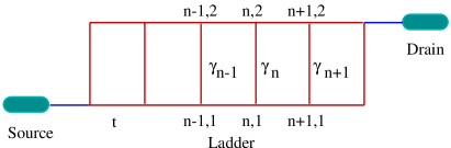
Figure 1: (Color online). Schematic view of a ladder attached to two electrodes.

variation in the conductance of the network, which may even exhibit a crossover from a completely opaque to a fully or partly transmitting one, is easily understood. In view of such a crossover one can then set the Fermi energy at a suitable energy zone in the spectrum and control the transmission characteristics. This enhances the prospect of such ladder networks as novel switching devices. The possibility of designing DNA devices, to our mind, can also be encouraged by such analysis. Our results are exact. Finally, we present numerical results for a quasiperiodically ordered ladder network by evaluating the two terminal conductance within a Green’s function formalism. The conductance spectrum not only corroborates the general features of disordered networks discussed previously and as revealed in our analytical approach, but also shows the presence of localization-de-localization transition in the quasiperiodic ladder network. Again in this case, analytical results may be obtained by appropriately adjusting the system parameters.

Let us refer to Fig. 1. The Hamiltonian of the ladder network is given by,

$${\mathbf{H}}=\sum_{n}{\bf{\epsilon_{n}c_{n}^{\dagger}c_{n}}}+{\mathbf{t}}\sum_{n}{\mathbf{c}_{n}^{\dagger}c_{n+1}}+h.c.$$ (1)

where,

$${\bf c_{n}}=\left(\begin{array}[]{c}c_{n,1}\\ c_{n,2}\end{array}\right)$$ (2)

In the above, $c_{n,j}$ ($c_{n,j}^{\dagger}$) are the annihilation (creation) operator at the $n$th site of the $j$th ladder.

$$\bf{\epsilon_{n}} = \left(\begin{array}[]{cc}\epsilon_{n,1}&\gamma_{n}\\ \gamma_{n}&\epsilon_{n,2}\end{array}\right)$$ (5)

$$\bf{t} = \left(\begin{array}[]{cc}t&0\\ 0&t\end{array}\right)$$ (8)

where $\epsilon_{n,j}$ is the on-site potential at the $n$th site of the $j$th ladder, $\gamma_{n}$ is the vertical hopping between the $n$th sites of the two arms of the ladder and, $t$ is the nearest-neighbor hopping integral between the $n$th and the ($n+1$)th sites of every arm.

We describe the system in a basis defined by the vector

$${\bf f_{n}}=\left(\begin{array}[]{c}f_{n,1}\\ f_{n,2}\end{array}\right)$$ (9)

where, $f_{n,j}$ is the amplitude of the wave function at the $n$th site of the $j$th arm of the ladder, $j$ being equal to $1$ or $2$. Using this basis, our task is to obtain solutions of the difference equation

$$(E{\bf I}-{\bf\epsilon_{n}}){\mathbf{f}_{n}}={\bf t}({\bf f_{n+1}}+{\bf f_{n-1}})$$ (10)

$I$ being the $2\times 2$ identity matrix. Let us now separately discuss cases which will throw light on the central problem addressed in this paper, viz, the possibility of getting a localization-delocalization transition in such a system. Case I: $\epsilon_{n,2}=\epsilon\epsilon_{n,1}$ and, $\gamma_{n}=\gamma\epsilon_{n,1}$. We introduce the above correlation between the on-site potentials at each arm. The selection of $\epsilon_{n,1}$ is of course, done in a random manner. With this choice of the parameters, the difference equation ($5$) reads,

$$\left[E{\bf I}-\epsilon_{n,1}{\bf M}\right]{\bf f_{n}}=t{\bf I}\left({\bf f_{n+1}}+{\bf f_{n-1}}\right)$$ (11)

where,

$$\bf{M} = \left(\begin{array}[]{cc}1&\gamma\\ \gamma&\epsilon\end{array}\right)$$ (14)

We now diagonalize the matrix $\bf{M}$ by a similarity transformation using a matrix $\bf{S}$, and define

$${\bf\phi_{n}}={S^{-1}}{\bf f_{n}}$$ (15)

The above difference equation ($6$) now decouples, in this new basis, in the following pair of equations,

$$(E-\lambda_{1}\epsilon_{n,1})\phi_{m,1}=t(\phi_{n+1,1}+\phi_{n-1,1})$$ (16)

$$(E-\lambda_{2}\epsilon_{n,1})\phi_{n,2}=t(\phi_{n+1,2}+\phi_{n-1,2})$$ (17)

Here, $\phi_{n,1}$ and $\phi_{n,2}$ are the elements of the column vector ${\bf\phi_{n}}$ and, $\lambda_{1}$ and $\lambda_{2}$ are the eigenvalues of the matrix $\bf{M}$ which are given by,

$$\lambda_{1} = \frac{1+\epsilon}{2}+\sqrt{\left[\left(\frac{1-\epsilon}{2}\right)^{2}+\gamma^{2}\right]}$$

$$\lambda_{2} = \frac{1+\epsilon}{2}-\sqrt{\left[\left(\frac{1-\epsilon}{2}\right)^{2}+\gamma^{2}\right]}$$ (18)

We can now extract information about the nature of eigenfunctions of the original ladder network in different parametric and energy space by considering the two Eqs. (16) and (17) simultaneously.

Figure 2: (Color online). Schematic view of a ladder attached to two electrodes, where each arm of the ladder is a Fibonacci chain.

First of all, for any fixed value of $\epsilon$, the set of equations ($9$) and ($10$) together defines a ladder network consisting of random on-site potentials occupying the arms $1$ and $2$. As both these equations represent randomly disordered one dimensional chains, one expects Anderson localization of all the electronic states provided $\lambda_{1}$ and $\lambda_{2}$ are non-zero. The states of the ladder network will be exponentially localized. However, there is a point of interest.

It is well known that, for a randomly disordered chain of length $L$ with $L>>1$, but not very large, one encounters a distribution of localization lengths. The distribution is characterized by ‘local’ Lyapunov exponents which can be different for different eigenstates of the disordered sample tosatti . Only in the thermodynamic limit one single exponent dominates the distribution and one can talk of a ‘unique’ characteristic localization length. In the case of a ladder of large but finite length Eqs. (16) and (17) represent chains having two different widths of disorder and hence, two different distributions of localization lengths. One can however, simulate the thermodynamic limit by averaging over various disorder configurations. As a result of such averaging the ‘distribution’ of localization lengths will be dominated by one Lyapunov exponent, and we can talk of a characteristic localization length of the disordered sample. Assuming this is done, the Eqs. (16) and (17) will represent chains with two different (characteristic) lengths of localization.

Let $\xi_{1}$ and $\xi_{2}$ be these characteristic localization lengths corresponding to Eqs. (16) and (17) respectively, and let’s set, without any loss of generality, $\xi_{1}<L<\xi_{2}$. As the Fermi energy is swept through the eigenvalue spectrum corresponding to Eq. (16), the ladder doesn’t conduct, as $L>\xi_{1}$. On the other hand, as the Fermi energy coincides with any of the eigenvalues corresponding to the spectrum provided by Eq. (17), the ladder shows a finite conductance. Thus, the finite ladder exhibits a transition from a non-conducting to a conducting phase and thus shows a switch-like behavior. Of course, the value of the conductance in the second case may not always be high. Case II: $\epsilon_{n,1}$ are random, $\epsilon_{n,2}=\epsilon\epsilon_{n,1}$ and $\gamma_{n}=\gamma\epsilon_{n,1}$, such that $\lambda_{2}=0$. This implies, $\gamma_{n}=\sqrt{(\epsilon_{n,1}\epsilon_{n,2})}$. For this special choice of the parameters, Eqs. (16) and (17) read,

$$[E-(\epsilon_{n,1}+\epsilon_{n,2})]\phi_{n,1}=t(\phi_{n+1,1}+\phi_{n-1,1})$$ (19)

$$E\phi_{n,2}=t(\phi_{n+1,2}+\phi_{n-1,2})$$ (20)

This is an interesting case. Eq. (19) represents the eigenvalue equation for a disordered chain with $\epsilon_{n,1}$ being uncorrelated random potentials. Therefore, the electronic states represented by $\phi_{n,1}$ are exponentially localized. On the other hand, Eq. (20) represents a perfectly ordered chain with on-site potential being equal to zero at each site. All the eigenstates represented by $\phi_{n,2}$ are extended and the system represented by the set of Eqs. (20) has an absolutely continuous energy spectrum ranging from $E=-2t$ to $E=2t$ in the thermodynamic limit. This implies that, in the actual system, all the states beyond $|E|=2t$ will be localized exponentially (courtesy, Eq. (19)) and we get mobility edges at $E=\pm 2t$. This presents an example where the existence of mobility edges can be proven analytically in a low dimensional disordered system, such as a two-chain ladder discussed here. Case III: A Fibonacci ladder Let us now discuss a quasiperiodic version of the ladder, viz, a Fibonacci ladder. Each arm of the ladder is a quasiperiodic Fibonacci chain kohmoto . A binary Fibonacci chain is composed of two ‘letters’ $A$ and $B$ and the consecutive Fibonacci generations are grown following the substitution rules, $A\rightarrow AB$ and $B\rightarrow A$ with $A$ as the seed kohmoto . The on-site potentials now assume values $\epsilon_{A,j}$ and $\epsilon_{B,j}$ for an $A$-type or a $B$-type vertex in the ladder, $j$ being the arm-index. The variety of vertices makes the inter-ladder hopping $\gamma_{n}$ take up values $\gamma_{A}$ or $\gamma_{B}$ depending on whether it connects the $A-A$ vertices or the $B-B$ vertices in the ladder in the transverse direction (Fig. 2).

We first discuss a special case again, in the spirit of our earlier Case I. We choose $\epsilon=0$ and $\gamma_{n}=\gamma\epsilon_{n,1}$. It implies, $\epsilon_{n,2}=\epsilon\epsilon_{n,1}=0$, but the ladder still retains its quasiperiodic Fibonacci character. Eq. (16) and Eq. (17) retain their forms, but now with $\lambda_{1}=(1+\sqrt{1+4\gamma^{2}})/2$ and, $\lambda_{2}=(1-\sqrt{1+4\gamma^{2}})/2$. As $\epsilon_{n,1}$ is taken to be distributed in a Fibonacci sequence along arm number one of the ladder, each of the equations (16) and (17) represents equations for two independent Fibonacci chains. The eigenstates for each of them are typically critical kohmoto , exhibiting power law localization with a multifractal distribution of the exponents. Thus, the spectrum of the Fibonacci ladder will be composed only of such critical states and no question of localization-delocalization transition arises.

Now, as a second case, we select $\epsilon_{A,2}=\epsilon_{A,1}$ and, $\epsilon_{B,2}=\epsilon_{B,1}$, $\gamma_{A}=\sqrt{(\epsilon_{A,1}\epsilon_{A,2})}=\epsilon_{A,1}$ and $\gamma_{B}=\sqrt{(\epsilon_{B,1}\epsilon_{B,2})}=\epsilon_{B,1}$, which automatically makes $\epsilon=1$ and $\gamma=1$. The same set of Eqs. (19) and (20) are obtained. Now, $\epsilon_{n,1}+\epsilon_{n,2}$ is either $2\epsilon_{A}$ or $2\epsilon_{B}$. That is, Eq. (19) represents a one dimensional Fibonacci chain for all the single particle states are critical

Figure 3: (Color online). $g$-$E$ (red color) and $\rho$-$E$ (blue color) curves for a ladder of total number of rungs $34$. (a) one chain (chain number $2$) is ordered with on-site potential set equal to unity and the other chain (chain number $1$) is subjected to Fibonacci modulation in site energies with $\epsilon_{A,1}=-4$ and $\epsilon_{B,1}=4$ (b) both the chains are subjected to Fibonacci modulation in site energies with $\epsilon_{A,1}=\epsilon_{A,2}=-4$ and $\epsilon_{B,1}=\epsilon_{B,2}=4$. Other parameters are, $t_{l}=3$, $\gamma=3$, and the on-site potential and the hopping integral in the electrodes are set as $\epsilon_{0}=0$ and $t_{0}=4$ respectively. We have chosen $c=e=h=1$.

kohmoto and the spectrum in the thermodynamic limit, is a Cantor set, with a gap in the neighborhood of every energy. The central part of the spectrum of course, remains extended by virtue of Eq. (20), refers to a perfectly ordered chain of atoms. Thus we again come across mobility edges beyond $|E|=2t$, but now its a transition from extended to critical (power-law localized) states. The conductance accordingly drops from (relatively) high to low values as one crosses such mobility edges.

For a Fibonacci chain without the above restrictive values of the parameters, we have to resort to numerical methods. Without any specified correlation between the on-site potentials in the arms or in the values of the inter-arm hopping $\gamma$, the decoupling of the ladder network into two independent one dimensional chains is not possible (this is of course, true even with the disordered ladder). However, the analysis made so far does not rule out the possibility of a metal-insulator transition even in a general case. As an example, we have performed a numerical calculation of the density of states $\rho$ and conductance $g$ of a finite Fibonacci ladder. Results for two separate cases are shown in Fig. 3. In the first case, one arm is an ordered chain while the other arm has a quasiperiodic Fibonacci distribution of the on-site potentials. In the second case, both the arms have a Fibonacci character.

For the numerical calculation we have adopted a Green’s function formalism. A finite ladder is attached to two semi-infinite one-dimensional perfect electrodes, viz, source and drain, described by the standard tight-binding Hamiltonian and parametrized by constant on-site potential $\epsilon_{0}$ and nearest neighbor hopping integral $t_{0}$ (already illustrated in Fig. 1). For low bias voltage and temperature, the conductance $g$ of the ladder is determined by the single channel Landauer conductance formula datta $g=(2e^{2}/h)T$. The transmission probability $T$ is given by datta $T=Tr\left[\Gamma_{S}G_{L}^{r}\Gamma_{D}G_{L}^{a}\right]$. $\Gamma_{S}$ and $\Gamma_{D}$ correspond to the imaginary parts of the self-energies due to coupling of the ladder with the two electrodes and $G_{L}$ represents the Green’s function of the ladder new ; muj1 ; muj2 .

In Fig. 3 we have superposed the picture of the density of states on the conductance profile to show clearly that we have eigenstates existing in energy regimes for which the conductance is very low. This illustrates the transition from the conducting (high $g$) to non-conducting phase.

In conclusion, the results presented in this communication are worked out for zero temperature. However, they should remain valid even in a certain range of finite temperatures ($\sim 300$ K). This is because the broadening of the energy levels of the ladder due to the electrode-ladder coupling is, in general, much larger than that of the thermal broadening datta . The inter ladder hopping $\gamma$ shifts the spectra corresponding to Eqs. (19) and (20) relative to each other. As a result, in principle, one can tune the positions of the mobility edges. This aspect may be inspiring in designing low-dimensional switching devices, or even a DNA device.

References

- (1) P. W. Anderson, Phys. Rev. 109, 1492 (1958).
- (2) P. A. Lee and T. V. Ramakrsihnan, Rev. Mod. Phys. 57, 287 (1985), and references therein.
- (3) E. Abrahams, P. W. Anderson, D. C. Licciardello, and T. V. Ramakrishnan, Phys. Rev. Lett. 42, 673 (1979).
- (4) S. Aubry and G. André, in Group Theoretical Methods in Physics, edited by L. Horwitz and Y. Neeman, Annals of the Israel Physical Society Vol. 3 (American Institute of Physics, New York, 1980), p. 133.
- (5) C. M. Soukoulis and E. N. Economou, Phys. Rev. Lett. 48, 1043 (1982).
- (6) S. Das Sarma, Song He, and X. C. Xie, Phys. Rev. Lett. 61, 2144 (1988).
- (7) S. Das Sarma, Song He, and X. C. Xie, Phys. Rev. B 41, 5544 (1990).
- (8) M. Johansson and R. Riklund, Phys. Rev. B 42, 8244 (1990).
- (9) M. Johansson and R. Riklund, Phys. Rev. B 43, 13468 (1991) .
- (10) D. H. Dunlap, H.-L. Wu, and P. Phillips, Phys. Rev. Lett. 65, 88 (1990); A. Bovier, J. Phys. A 25, 1021 (1992); J. C. Flores and M. Hilke, J. Phys. A 26, L1255 (1993).
- (11) A. Sánchez, E. Maciá, and F. Domínguez-Adame, Phys. Rev. B 49, 147 (1994).
- (12) F. A. B. F. de Moura and M. L. Lyra, Phys. Rev. Lett. 81, 3735 (1998); F. M. Izrailev and A. A. Krokhin, Phys. Rev. Lett. 82, 4062 (1999).
- (13) F. Domínguez-Adame, V. A. Malyshev, F. A. B. F. de Moura, and M. L. Lyra, Phys. Rev. Lett. 91, 197402 (2003).
- (14) E. Maciá, Phys. Rev. B 74, 245105 (2006).
- (15) G. Cuniberti, E. Maciá, A. Rodriguez, and R. A. Römer, in Charge Migration in DNA: Perspectives from Physics, Chemistry and Biology, edited by T. Chakraborty (Springer-Verlag, Berlin, 2007), pp. 1-21.
- (16) R. A. Caetano and P. A. Schulz, Phys. Rev. Lett. 95, 126601 (2005).
- (17) S. Sil, S. K. Maiti, and A. Chakrabarti, Phys. Rev. Lett. 101, 076803 (2008).
- (18) L. Pietronero, A. P. Siebesma, E. Tosatti, and M. Zanetti, Phys. Rev. B 36, 5635 (1987).
- (19) M. Kohmoto, L. P. Kadanoff, and C. Tang, Phys. Rev. Lett. 50, 1870 (1983); M. Kohmoto, B. sutherland, and C. Tang, Phys. Rev. B 35, 1020 (1987).
- (20) S. Datta, Electronic transport in mesoscopic systems, Cambridge University Press, Cambridge (1997).
- (21) D. M. Newns, Phys. Rev. 178, 1123 (1969).
- (22) V. Mujica, M. Kemp, and M. A. Ratner, J. Chem. Phys. 101, 6849 (1994).
- (23) V. Mujica, M. Kemp, A. E. Roitberg, and M. A. Ratner, J. Chem. Phys. 104, 7296 (1996).