The Physics of Wind-Fed Accretion

Abstract

We provide a brief review of the physical processes behind the radiative driving of the winds of OB stars and the Bondi-Hoyle-Lyttleton capture and accretion of a fraction of the stellar wind by a compact object, typically a neutron star, in detached high-mass X-ray binaries (HMXBs). In addition, we describe a program to develop global models of the radiatively-driven photoionized winds and accretion flows of HMXBs, with particular attention to the prototypical system Vela X-1. The models combine XSTAR photoionization calculations, HULLAC emission models appropriate to X-ray photoionized plasmas, improved models of the radiative driving of photoionized winds, FLASH time-dependent adaptive-mesh hydrodynamics calculations, and Monte Carlo radiation transport. We present two- and three-dimensional maps of the density, temperature, velocity, ionization parameter, and emissivity distributions of representative X-ray emission lines, as well as synthetic global Monte Carlo X-ray spectra. Such models help to better constrain the properties of the winds of HMXBs, which bear on such fundamental questions as the long-term evolution of these binaries and the chemical enrichment of the interstellar medium.

1 Introduction

As described by Castor, Abbott, and Klein (hereafter CAK) cak75 , mass loss in the form of a high-velocity wind is driven from the surface of OB stars by radiation pressure on a multitude of resonance transitions of intermediate charge states of cosmically abundant elements. The wind is characterized by a mass-loss rate $\dot{M}\approx 10^{-6}$–$10^{-5}~{}M_{\odot}~{}\rm yr^{-1}$ and a velocity profile $v(r)\approx v_{\infty}(1-R_{\star}/r)^{\beta}$, where $r$ is the distance from the OB star, $\beta\approx\frac{1}{2}$, $v_{\infty}\approx 3v_{\rm esc}$ is the terminal velocity, $v_{\rm esc}=(2GM_{\star}/R_{\star})^{1/2}$ is the escape velocity, and $M_{\star}$ and $R_{\star}$ are respectively the mass and radius of the OB star. As described by Hoyle and Lyttleton hoy39 , Bondi bon52 , and Shapiro and Lightman sha76 , in detached high-mass X-ray binaries (HMXBs), a compact object, typically a neutron star, captures the fraction of the wind of the OB star that passes within the accretion radius $r_{\rm a}=\zeta 2GM_{\rm x}/v_{\rm rel}^{2}$ of the compact object, where $\zeta$ is a constant of order unity, $v_{\rm rel}=(v_{\rm w}^{2}+v_{\rm x}^{2})^{1/2}$ is the velocity of the wind relative to the compact object, $v_{\rm w}$ is the velocity of the wind at $r=a$, $v_{\rm x}=2\pi a/P_{\rm orb}$ is the orbital velocity of the compact object, $a=[G(M_{\star}+M_{\rm x})(P_{\rm orb}/2\pi)^{2}]^{1/3}$ is the binary separation, and $P_{\rm orb}$ is the binary orbital period. The mass-accretion rate onto the compact object $\dot{M}_{\rm a}=\pi r_{\rm a}^{2}\rho_{\rm w}v_{\rm rel}$, where $\rho_{\rm w}=\dot{M}_{\rm w}/4\pi a^{2}v_{\rm w}$ is the wind mass density and $\dot{M}_{\rm w}$ is the wind mass-loss rate, hence $\dot{M}_{\rm a}=\frac{1}{4}\,(r_{\rm a}/a)^{2}(v_{\rm rel}/v_{\rm w})\dot{M}_{\rm w}\equiv f\dot{M}_{\rm w}$. This compact expression expands out to

$$\dot{M}_{\rm a}\approx 0.012\,\zeta^{2}\eta^{-4}(M_{\rm x}/M_{\odot})^{2}(M_{\star}/M_{\odot})^{-8/3}(R_{\star}/R_{\odot})^{2}(P_{\rm orb}/{\rm d})^{-4/3}\dot{M}_{\rm w},$$ (1)

where $\eta\equiv(v_{\rm w}/v_{\rm esc})\approx 3\,(1-R_{\star}/a)^{\beta}$ for an isolated OB star. For the parameters appropriate to the prototypical detached HMXB Vela X-1 (§2), $\dot{M}_{\rm a}\approx 7\times 10^{-5}\dot{M}_{\rm w}\sim 7\times 10^{-11}~{}M_{\odot}~{}\rm yr^{-1}$. Accretion of this material onto the neutron star powers an X-ray luminosity $L_{\rm x}=G\dot{M}_{\rm a}M_{\rm x}/R_{\rm x}\sim 1\times 10^{36}~{}{\rm erg~{}s}^{-1}$, where $M_{\rm x}$ and $R_{\rm x}$ are respectively the mass and radius of the compact object. The resulting X-ray flux photoionizes the wind and reduces its ability to be radiatively driven, both because the higher ionization state of the plasma results in a reduction in the number of resonance transitions, and because the energy of the transitions shifts to shorter wavelengths where the overlap with the stellar continuum is lower. To first order, the lower radiative driving results in a reduced wind velocity $v_{\rm w}$ near the compact object, which increases the accretion radius $r_{\rm a}$, which increases the accretion efficiency $f$, which increases the X-ray luminosity $L_{\rm x}$. In this way, the X-ray emission of HMXBs is the result of a complex interplay between the radiative driving of the wind of the OB star and the photoionization of the wind by the neutron star.

Known since the early days of X-ray astronomy, HMXBs have been extensively studied observationally, theoretically hat77 ; mcc84 ; ste90 , and computationally blo90 ; blo91 ; blo94 ; blo95 . They are excellent targets for X-ray spectroscopic observations because the large covering fraction of the wind and the moderate X-ray luminosities result in large volumes of photoionized plasma that produce strong recombination lines and narrow radiative recombination continua of H- and He-like ions, as well as fluorescent lines from lower charge states.

Figure 1: Three views of the Chandra HETG Medium Energy Grating count spectrum of Vela X-1 in eclipse, with the strongest emission features labeled: (a) the broad 0.7–10 keV bandpass, (b) the line-rich 4–15 Å bandpass, and (c) the 6.1–7.3 Å bandpass containing emission lines from H- and He-like Si as well as fluorescence emission features from L-shell Si.

2 Vela X-1

The prototypical detached HMXB Vela X-1 has been studied extensively in nearly every waveband, particularly in X-rays, since its discovery as an X-ray source during a rocket flight four decades ago. It consists of a B0.5 Ib supergiant and a magnetic neutron star in an 8.964-day orbit. From an X-ray spectroscopic point of view, Vela X-1 distinguished itself in 1994 when Nagase et al. nag94 , using ASCA SIS data, showed that, in addition to the well-known 6.4 keV Fe K$\alpha$ emission line, the eclipse X-ray spectrum is dominated by recombination lines and continua of H- and He-like Ne, Mg, Si, S, Ar, and Fe. These data were subsequently modeled in detail by Sako et al. sak99 , using a kinematic model in which the photoionized wind was characterized by the ionization parameter $\xi\equiv L_{\rm x}/nR^{2}$, where $R$ is the distance from the neutron star and $n$ is the number density, given by the mass-loss rate and velocity law of an undisturbed CAK wind [specifically, $n=\dot{M}_{\rm w}/4\pi\mu v(r)r^{2}$, where $\mu$ is the mean atomic weight and $v(r)=v_{0}+v_{\infty}(1-R_{\star}/r)^{\beta}$]. Vela X-1 was subsequently observed with the Chandra High Energy Transmission Grating (HETG) in 2000 for 30 ks in eclipse sch02 and in 2001 for 85, 30, and 30 ks in eclipse and at binary phases 0.25 and 0.5, respectively gol04 ; wat06 ; three views of the line-rich eclipse spectrum are shown in Figure 1. Watanabe et al. wat06 , using assumptions very similar to those of Sako et al. and a Monte Carlo radiation transfer code, produced a global model of Vela X-1 that simultaneously fits the HETG spectra from the three binary phases with a wind mass-loss rate $\dot{M}_{\rm w}\approx 2\times 10^{-6}~{}M_{\odot}~{}\rm yr^{-1}$ and terminal velocity $v_{\infty}=1100~{}\rm km~{}s^{-1}$. One of the failures of this model was the velocity shifts of the emission lines between eclipse and binary phase 0.5, which were observed to be $\Delta v\approx 400$–$500~{}\rm km~{}s^{-1}$, while the model simulations predicted $\Delta v\sim 1000~{}\rm km~{}s^{-1}$. In order to resolve this discrepancy, Watanabe et al. performed a 1-dimensional calculation to estimate the wind velocity profile along the line of centers between the two stars, accounting, in an approximate way, for the reduction of the radiative driving due to photoionization. They found that the velocity of the wind near the neutron star is lower by a factor of 2–3 relative to that of an undisturbed CAK wind, which was sufficient to explain the observations. However, these results were not fed back into their global model to determine the effect on the X-ray spectra. Equation 1 suggests that, for a given wind mass-loss rate, the X-ray luminosity should be higher by a factor of (2–$3)^{4}=16$–81, or, for a given X-ray luminosity, that the wind mass-loss rate should be lower by a similar factor.

3 Hydrodynamic Simulations

To make additional progress in our understanding of the wind and accretion flow of HMXBs in general and Vela X-1 in particular — to combine the best features of the hydrodynamic models of Blondin et al. blo90 ; blo91 ; blo94 ; blo95 and the kinematic-spectral models of Sako et al. sak99 and Watanabe et al. wat06 — we have undertaken a project to develop improved models of radiatively-driven photoionized accretion flows, with the goal of producing synthetic X-ray spectra that possess a level of detail commensurate with the grating spectra returned by Chandra and XMM-Newton. This project combines:

• XSTAR kal01 photoionization calculations, which provide the heating $\Gamma$ and cooling $\Lambda$ rates of the plasma and the ionization fractions of the various ions as a function of temperature $T$ and ionization parameter $\xi$.

• HULLAC bar88 emission models appropriate to X-ray photoionized plasmas.

• Improved models of the radiative driving of the photoionized wind.

• FLASH fry00 two- and three-dimensional time-dependent adaptive-mesh hydrodynamics calculations.

• Monte Carlo radiation transport mau04 .

Radiative driving of the wind is accounted for via the force multiplier formalism cak75 , wherein the radiative acceleration $g_{\rm rad}=g_{\rm e}\,(1+M)$, where $g_{\rm e}=\kappa_{\rm e}L_{\star}/4\pi r^{2}c$ is the radiative acceleration due to electron (Thomson) scattering; $\kappa_{\rm e}=n_{\rm e}\sigma_{\rm T}/\rho\approx 0.34~{}\rm cm^{2}~{}g^{-1}$ is the Thomson opacity; $n_{\rm e}$ is the electron number density; $\rho$ is the mass density; $M=\sum_{\rm lines}(F_{\nu}/F)(v_{\rm th}\nu/c)(1-e^{-\eta t})/t$ is the line force multiplier; $v_{\rm th}=(2kT_{\star}/m_{\rm p})^{1/2}$ is the mean thermal velocity of the protons; $T_{\star}$, $L_{\star}$, and $F_{\nu}/F$ are respectively the effective temperature, luminosity, and normalized flux distribution of the OB star; $t=\kappa_{\rm e}v_{\rm th}\rho(dv/dr)^{-1}$ is the optical depth parameter; $dv/dr$ is the velocity gradient; $\eta$ accounts for all the atomic physics (wavelengths, oscillator strengths, statistical weights, and fractional level populations); and the other symbols have their usual meanings. We calculated $M[T,\xi,t]$ on a $[21\times 51\times 41]$ lattice accounting for X-ray photoionization and non-LTE population kinetics using HULLAC atomic data for $2\times 10^{6}$ lines of $35{,}000$ energy levels of 166 ions of the 13 most cosmically abundant elements. Compared to Stevens and Kallman ste90 , our line force multipliers are typically higher at low $t$ because of the larger number of lines in our models, and lower at high $t$ because we do not assume that the level populations are in LTE.

In addition to the usual hydrodynamic quantities, the FLASH calculations account for:

• The gravity of the OB star and neutron star (although, following Ruffert ruf94 , for numerical reasons we softened the gravitational potential of the neutron star over a scale length $\epsilon=10^{3}\,R_{\rm x}=10^{9}$ cm).

• Coriolis and centrifugal forces.

• Radiative driving of the wind as a function of the local ionization parameter, temperature, and optical depth.

• Photoionization and Compton heating of the irradiated wind.

• Radiative cooling of the irradiated wind and the “shadow wind” behind the OB star.

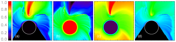
Figure 2: Color-coded maps of (a) $\log T\,({\rm K})=[4.4,8.3]$, (b) $\log n\,({\rm cm}^{-3})=[7.4,10.8]$, (c) $\log v\,({\rm km~{}s^{-1}})=[1.3,3.5]$, and (d) $\log\xi\,({\rm erg~{}cm~{}s^{-1}})=[1.1,7.7]$ in the orbital plane of Vela X-1. The positions of the B star and neutron star are shown by the circle and the “$\times$,” respectively. The horizontal axis $x=[-5,7]\times 10^{12}$ cm and the vertical axis $y=[-4,8]\times 10^{12}$ cm.

4 2D Hydrodynamic Simulations

To demonstrate typical results of our simulations, we show in Fig. 2 color-coded maps of the log of the (a) temperature $T$, (b) density $n$, (c) velocity $v$, and (d) ionization parameter $\xi$ of a FLASH 2-dimensional simulation in the binary orbital plane of an HMXB with parameters appropriate to Vela X-1 (specifically, those of Sako et al. sak99 ). In this simulation, the computational volume $x=[-5,7]\times 10^{12}$ cm and $y=[-4,8]\times 10^{12}$ cm, the B star is centered at $[x,y]=[0,0]$, the neutron star is centered at $[x,y]=[0,3.7\times 10^{12}]$ cm, and $128\times 128=16{,}384$ computational cells were used for a spatial resolution of $\Delta l=9.4\times 10^{10}$ cm. At the time step shown ($t=100$ ks), the relatively slow ($v\approx 400~{}\rm km~{}s^{-1}$) irradiated wind has reached just $\sim 2$ stellar radii from the stellar surface. The various panels show (1) the effect of the Coriolis and centrifugal forces, which cause the flow to curve clockwise, (2) the cool, fast wind behind the B star, (3) the hot, slow, irradiated wind, (4) the hot, low-density, high-velocity flow downstream of the neutron star, and (5) the bow shock and two flanking shocks formed where the irradiated wind collides with the hot disturbed flow in front and downstream of the neutron star.

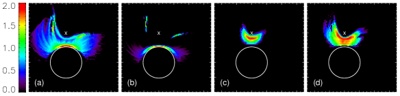
Figure 3: Similar to Fig. 2, but for the log of the X-ray emissivity of (a) Si XIV Ly$\alpha$, (b) Si XIII He$\alpha$, (c) Fe XXVI Ly$\alpha$, and (d) Fe XXV He$\alpha$ in the orbital plane of Vela X-1. In each case, two orders of magnitude are plotted.

Given these maps, it is straightforward to determine where in the binary the X-ray emission originates. To demonstrate this, we show in Fig. 3 color-coded maps of the log of the emissivity of (a) Si XIV Ly$\alpha$, (b) Si XIII He$\alpha$, (c) Fe XXVI Ly$\alpha$, and (d) Fe XXV He$\alpha$. The gross properties of these maps are consistent with Fig. 24 of Watanabe et al., but they are now (1) quantitative rather than qualitative and (2) specific to individual transitions of individual ions. The maps also capture features that otherwise would not have been supposed, such as the excess emission in the H- and He-like Si lines downstream of the flanking shocks. Combining these maps with the velocity map (Fig. 2c), these models make very specific predictions about the intensity of the emission features, where they originate, and their velocity widths and amplitudes as a function of binary phase.

5 3D Hydrodynamic Simulations

Having developed and extensively tested our software on various 2-dimensional simulations, we next calculated a more limited number of 3-dimensional simulations of an HMXB with parameters appropriate to Vela X-1. Figure 4 shows, for one of these simulations, the log of the number density on three orthogonal planes passing through the computational volume, which spans $\Delta x=12\times 10^{12}$ cm, $\Delta y=16\times 10^{12}$ cm, and $\Delta z=8\times 10^{12}$ cm using $192\times 256\times 128=6.3\times 10^{6}$ computational cells, for a spatial resolution $\Delta l=6.3\times 10^{10}$ cm. In order to compare our hydrodynamic calculations to the kinematic models of Sako et al. sak99 and Watanabe et al. wat06 , we also calculated, on the same 3-dimensional grid, using the parameters of Watanabe et al., the velocity $v(r)=v_{0}+v_{\infty}(1-R_{\star}/r)^{\beta}$, density $n=\dot{M}_{\rm w}/4\pi\mu v(r)r^{2}$, and ionization parameter $\xi\equiv L_{\rm x}/nR^{2}$ for an assumed undisturbed CAK wind, assuming that the temperature $T(\xi)$ is that of a photoionized plasma in thermal equilibrium: $\Gamma(T,\xi)=\Lambda(T,\xi)$. Figure 1 of Akiyama et al. aki07 shows color-coded maps in the binary orbital plane of the density and temperature and the Si XIV and Fe XXVI ion abundances for the CAK and FLASH models, emphasizing the dramatic differences between them.

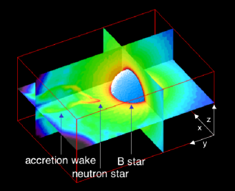
Figure 4: Color-coded maps of $\log n\,({\rm cm}^{-3})=[7.4,12.1]$ on three orthogonal planes from a FLASH 3D simulation of Vela X-1, showing the B star (blue sphere), neutron star, and accretion wake. The computational volume $x=[-6,6]\times 10^{12}$ cm, $y=[-6,10]\times 10^{12}$ cm, and $z=[-4,4]\times 10^{12}$ cm.

6 Synthetic X-ray Spectra

In the next step in this process, we fed the physical parameters of the CAK and FLASH models into our Monte Carlo radiation transfer code and followed the spatial and spectral evolution of photons launched from the surface of the neutron star until they are either destroyed or escape the computational volume. As detailed by Mauche et al. mau04 , the Monte Carlo code accounts for Compton and photoelectric opacity of 446 subshells of 140 ions of the 12 most abundant elements. Following photoabsorption by K-shell ions, we generate radiative recombination continua (RRC) and recombination line cascades in a probabilistic manner using the recombination cascade calculations described by Sako et al. sak99 , with the shapes of the RRCs determined by the functional form of the photoionization cross sections and the local electron temperature. Fluorescence emission from L-shell ions is ignored, since it is assumed to be suppressed by resonant Auger destruction (however, see Fig. 1(c) and Liedahl lie05 ).

The synthetic spectra resulting from the Monte Carlo simulations are shown in Fig. 5. The upper histogram is the assumed (featureless) power-law spectrum emitted by the neutron star, while the synthetic spectra for the CAK and FLASH physical models are shown by the middle and lower histograms, respectively. While it is too early in the development of our program to draw any firm conclusions from these spectra (or from the differences between them), they demonstrate the type of results produced by our Monte Carlo code — X-ray spectra rich in emission lines and RRCs — and the type of differences between simple CAK and detailed hydrodynamic models, highlighting the importance of the details of the 3-dimensional model to the emitted spectra.

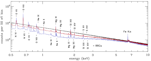
Figure 5: Monte Carlo X-ray spectra of the CAK (red) and FLASH (blue) models of Vela X-1 for the assumed power law neutron star X-ray spectrum (black). The H- and He-like ions responsible for the strongest emission lines and radiative recombination continua are indicated above and below the spectra, respectively.

We close by noting that Fig. 5 plots global X-ray spectra, irrespective of viewing angle or occultation by the B star, although it is straightforward to window the output of the Monte Carlo code to produce synthetic spectra for a specific viewing direction (for a given binary inclination and binary phase) or for a given binary inclination and a range of binary phases, and hence allow direct comparisons to actual data. The next step in our program is a careful comparison of such synthetic spectra to the grating spectra of Vela X-1 and other HMXBs returned by Chandra and XMM-Newton. In this way, it will be possible to better constrain the various parameters of the winds of HMXBs, such as the mass-loss rate $\dot{M}_{\rm w}$, terminal velocity $v_{\infty}$, velocity profile $v(r)$, and elemental abundances of the OB star — parameters that bear on such fundamental questions as the long-term evolution of these binaries and the chemical enrichment of the interstellar medium.

References

- (1) J. I. Castor, D. C. Abbott, and R. I. Klein, Ap.J., 195, 157 (1975), CAK.
- (2) F. Hoyle and R. A. Lyttleton, Proc. Cam. Phil. Soc., 35, 405 (1939).
- (3) Bondi, H., M. N. R. A. S., 112, 195 (1952)
- (4) S. L. Shapiro and A. P. Lightman, Ap.J., 204, 555 (1976).
- (5) S. Hatchett and R. McCray, Ap.J., 211, 552 (1977).
- (6) R. McCray, T. R. Kallman, J. I. Castor, and G. L. Olson, Ap.J., 282, 245 (1984).
- (7) I. R. Stevens and T. R. Kallman, Ap.J., 365, 321 (1990).
- (8) J. M. Blondin, T. R. Kallman, B. A. Fryxell, and R. E. Taam, Ap.J., 356, 591 (1990).
- (9) J. M. Blondin, I. R. Stevens, and T. R. Kallman, Ap.J., 371, 684 (1991).
- (10) J. M. Blondin, Ap.J., 435, 756 (1994).
- (11) J. M. Blondin and J. W. Woo, Ap.J., 445, 889 (1995).
- (12) F. Nagase, G. Zylstra, T. Sonobe, T. Kotani, H. Inoue, and J. Woo, Ap.J., 436, L1 (1994).
- (13) M. Sako, D. A. Liedahl, S. M. Kahn, and F. Paerels, Ap.J., 525, 921 (1999).
- (14) N. S. Schulz, C. R. Canizares, J. C. Lee, and M. Sako, Ap.J., 564, L21 (2002).
- (15) G. Goldstein, D. P. Huenemoerder, and D. Blank, A.J., 127, 2310 (2004).
- (16) S. Watanabe, et al., Ap.J., 651, 421 (2006).
- (17) T. Kallman and M. Bautista, Ap.J.S., 133, 221 (2001).
- (18) A. Bar-Shalom, M. Klapisch, and J. Oreg, Phys. Rev., A38, 1773 (1988).
- (19) B. Fryxell, et al., Ap.J.S., 131, 273 (2000).
- (20) C. W. Mauche, D. A. Liedahl, B. F. Mathiesen, M. A. Jimenez-Garate, and J. C. Raymond, Ap.J., 606, 168 (2004).
- (21) M. Ruffert, Ap.J., 427, 342 (1994).
- (22) S. Akiyama, C. W. Mauche, D. A. Liedahl and T. Plewa, Bull. A. A. S., 39, #20.03 (2007)
- (23) D. A. Liedahl, “Resonant Auger Destruction and Iron K Spectra in Compact X-ray Sources, in X-ray Diagnostics of Astrophysical Plasmas: Theory, Experiment, and Observation, edited by R. Smith, AIP Conference Proceedings 774, 2005, p. 99.