A Minimal Model for the Study of Polychronous Groups

Abstract

A minimal model of polychronous groups in neural networks is presented. The model is computationally efficient and allows the study of polychronous groups independent of specific neuron models. Computational experiments were performed with the model in one- and two-dimensional neural architectures to determine the dependence of the number of polychronous groups on various connectivity options. The possibility of using polychronous groups as computational elements is also discussed.

I Introduction

Significant progress has been made in understanding the human brain over the past half century. The behavior of individual neurons has been studied extensively, using both experimental and computational methods, to the point where science can explain not only the characteristics of the various neuron types within neural networks, but can also give a detailed account of the mechanisms within the neurons themselves that cause these behaviors. Despite this progress, there is still a huge gap in our understanding of how these low-level mechanisms eventually result in the high-level cognitive functions of the brain.

One phenomenon whose understanding may help bridge this gap is polychronization, an idea that was introduced by Izhikevich in 2006 Izhikevich (2006). In a network with interconnection delays, two neurons may fire at distinct times, yet have their spikes arrive at a common postsynaptic neuron simultaneously due to the difference in connection delays. This phenomenon is termed polychronization. In addition these neurons plus the stimulated postsynaptic neuron may have their output spikes arrive simultaneously at still other neurons, causing further neural activity. The set of neurons in this chain reaction is called a polychronous group, which we sometimes shorten to polygroup.

Polychronization is similar to the phenomenon of synfire chains Abeles (1991) Bienenstock (1995). However synfire chains appear when the neural network has synaptic connections with identical delay times, whereas polychronization occurs when there is a spectrum of connection delays between neurons, and is more like the idea of a synfire braid mentioned by Bienenstock. It has been suggested that synfire chains form the basis of learning in the neocortex Doursat and Bienenstock (2006), while others have explored the information processing aspects of such chains Claussen (2006). The focus of this paper is on neural networks with transmission delays between neurons, a necessary condition for the appearance of polychronization.

Precisely timed spatiotemporal patterns have been observed experimentally both in vivo and in vitro Rolston et al. (2007) Abeles et al. (1993). Although these experiments seem to provide evidence for the existence of polychronous groups in the brain, it is an open question as to whether such observed activity can be accounted for by surrogate data generation. While detection of polychronous groups in theoretical models is straightforward, the lack of full network data in experimental situations makes their observation problematic.

Izhikevich noted that the number of polychronous groups far exceeded the number of neurons in the systems he studied. This observation led him to hypothesize that polychronous groups may represent memories in the brain, which could possibly explain the rich diversity of brain behavior that seemingly transcends the capabilities of the neurons present.

In this paper we describe a simple neural network model that has a minimal number of features to support the study of polychronous groups. We also develop an associated algorithm for the calculation of polygroups formed in the model, and apply that algorithm to various random networks to determine the number of potential polygroups in these systems.

Additionally we describe a new form of neural computation using polychronous groups as the basic computational elements. The simultaneous firing of two polygroups can in some cases stimulate the formation of still other polychronous groups, leading to a cascade of activity extending far beyond the space and time of the initial neural firings. This combination of polygroups into new polygroups suggests a higher level structure to the dynamics of neural systems.

II Description of the model

II.1 Network model

In the original paper on polychronous groups, Izhikevich analyzed a network of neurons modeled individually by his own spiking neuron equations Izhikevich (2003); in addition, Spike Timing Dependent Plasticity (STDP) was used to adjust the weights in the network. Other researchers have also stressed the importance of STDP in forming such groups Hosaka et al. (2008) Izhikevich et al. (2004). While these features create a system that has certain characteristics of actual neurons in the brain, they are not necessary to study the phenomenon of polychronization. One of the key premises of this paper has been to abstract the system to the bare minimum features necessary for studying the pure computational concepts of polychronization and polychronous groups.

A simple digraph with connection delays is sufficient to model the essential features of polychronization. A neuron model that fires a spike when the sum of its inputs reaches a fixed threshold is used for the nodes of the digraph. Connections between neurons are lossless, and each has a fixed, integer delay associated with it. Discrete time is used in the model with the same integer scale. All connections are excitatory in the basic model.

The model assumes that if a neuron receives two or more simultaneous input spikes it will activate and fire its own spike. A system in which a single input spike causes a neuron to fire cannot be particularly interesting, since all that has happened in computational terms is that the spike has been delayed. Requiring a large number of simultaneous spikes for activation is more realistic in terms of modeling the human brain; it has been estimated that it takes 20 to 50 presynaptic spikes arriving within a short time window to cause a postsynaptic spike in the human brain Gerstner and Kistler (2002). However such a system would be far more difficult to analyze, and is simply not necessary for understanding the fundamentals of polychronization. Hence, requiring two spike arrivals is the simplest and most tractable arrangement that will yield computationally rich behavior.

To build a network in which to search for polychronous groups, we first choose $N$, the number of neurons in the network, and arrange these $N$ neurons in a circular array (i.e. a linear array with periodic boundary conditions). To choose the interconnections between these neurons two parameters are used, 1) a fixed number of input connections per neuron $m$, and 2) a radius $r$ of nearest neighbors of each neuron from which connections may be selected. When selecting input connections the neuron itself is excluded since we do not want self-connection. In our initial models, once the connections are set, each is assigned an integer delay chosen randomly from the range $[d_{min},d_{max}]$, where $d_{min}$ and $d_{max}$ are parameters of the model.

Notice that once the neural topology is fixed, the set of polychronous groups within the network is also fixed. The network itself can be studied to determine what polygroups are inherent within it, irrespective of any specific dynamic considerations.

An example of a polychronous group is depicted in figure 1. The vertical axis labels neurons and the horizontal axis shows time. The circles mark points at which specific neurons fire, and the lines show the travel of spikes from left to right from one neuron to another. In this example the two initiating neurons are neuron 1 which fires at t=0, and neuron 3 which fires at t=1. Spikes from these two neurons arrive at neuron 2 at time t=2, causing it to fire (this implies that the delay from neuron 1 to neuron 2 is 2 time units, and the delay from neuron 3 to neuron 2 is 1 time unit). Spikes from neuron 3 and neuron 2 arrive simultaneously at neuron 4, causing it to fire at t=3. Finally, spikes from neuron 1 and neuron 4 arrive at neuron 2 at t=4, causing it to fire again.

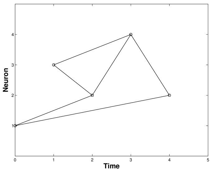
Figure 1: A depiction of an example of a polychronous group.

II.2 Finding Polychronous Groups

A polychronous group is determined by the indices of its two initiating neurons and the times at which they fire. The first step in our search for polygroups is to scan through each possible pair of neurons and examine each pair to see if it could initiate a polygroup with an appropriate choice of firing times. For a system with $N$ neurons we can form $N^{2}$ ordered pairs; however the neurons must be distinct and their order is unimportant, so the actual number of pairs we need to examine is $(N^{2}-N)/2$. For each pair of neurons we must also choose the times at which they fire. We are of course only interested in situations where these two neurons will cause another neuron to fire; for this to happen they must both have output connections to the same neuron. If such a common postsynaptic neuron exists, it is always possible to choose the initial firing times for the pair so that the postsynaptic neuron receives spikes from them simultaneously. The times are relative, allowing us to choose the earliest firing time to be $t=0$ and to choose the other time accordingly. For each pair of neurons being considered, we must examine all possible connection pairs for all common postsynaptic neurons.

The procedure above finds two neurons that stimulate a third neuron to fire, but by definition to have a polygroup at least one other neuron must also receive simultaneous spikes. The next step in the algorithm is to search for additional firings by allowing the system to evolve. The evolution of the system can be calculated efficiently by creating a matrix of spike arrival counts (see expression 1 below). The rows are numbered from 0 to $N-1$ corresponding to the $N$ neurons in the system; the columns are numbered from 0 to $t_{max}$, the maximum time to which the simulation is run. The matrix entry $q_{n,t}$ represents the number of spikes that arrive at neuron $n$ at time $t$. Initially we set all matrix entries to zero, except for the two initial nodes which we set to 2 at the appropriate times (this simulates these neurons receiving 2 input spikes, so that they will fire during the simulation run).

$$\left[\begin{array}[]{ccccc}q_{0,0}&q_{0,1}&\ldots&q_{0,t_{max}-1}&q_{0,t_{max}}\\ q_{1,0}&q_{1,1}&\ldots&q_{1,t_{max}-1}&q_{1,t_{max}}\\ \ldots&\ldots&\ddots&\ldots&\ldots\\ q_{N-2,0}&q_{N-2,0}&\ldots&q_{N-2,t_{max}-1}&q_{N-2,q_{0,t_{max}}}\\ q_{N-1,0}&q_{N-1,0}&\ldots&q_{N-1,t_{max}-1}&q_{N-1,q_{0,t_{max}}}\\ \end{array}\right]$$ (1)

To run the simulation we start at the leftmost column and look for entries with a value of 2 or greater. These neurons have received enough spikes to cause them to fire, so we look up what neurons they are connected to along with the associated delays to find the times at which the spikes arrive at the postsynaptic neurons. Using these numbers we find and increment the corresponding matrix entries. We then move to the second column and repeat the procedure.

The system can be run iteratively until no firings occur for a period of time equal to the maximum delay in the system. However in some cases polygroups can continue firing for a very long time; in fact, polygroups can extend infinitely in time. For this reason a limit is placed on how long the calculation will be performed. If the limit is reached the group is flagged as being overrun so that subsequent analysis can take this into account. At the end of the calculation, any matrix entry with a value of 2 or greater corresponds to a firing neuron. If there are four or more such entries, we have found a polygroup.

III Experimental Results

III.1 Results For One Dimensional Systems

The parameters of the experiment that can be varied are:

1. $N$ = number of neurons in the network.

2. $m$ = number of input connections per neuron.

3. $r$ = radius of nearest neighbors of each neuron from which connections may be chosen.

4. $d_{min}$ = minimum delay time.

5. $d_{max}$ = maximum delay time.

The first set of experiments was set up to determine how the number of polychronous groups varies as the the number of neurons in the system is changed, holding all other parameters constant. Figure 2 shows the results of these runs. For each value of $N$, 30 runs were averaged together to give the mean number of polychronous groups for that $N$. The relationship is clearly linear, with a slope of about 2.2. For these runs, $m=5$, $r=5$, $d_{min}=1$, and $d_{max}=5$.

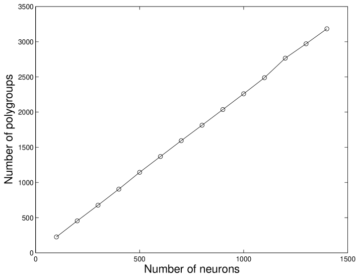
Figure 2: A plot showing the number of polychronous groups as a function of $N$, the number of neurons in the system.

For the next experiments we decided to determine how the number of polychronous groups varies as the the number of input connections to each neuron changes. Results are displayed in Figure 3, which shows that the number of polychronous groups increases rapidly as $m$ is increased. For these runs, $N=100$, $r=10$, $d_{min}=1$, and $d_{max}=5$.

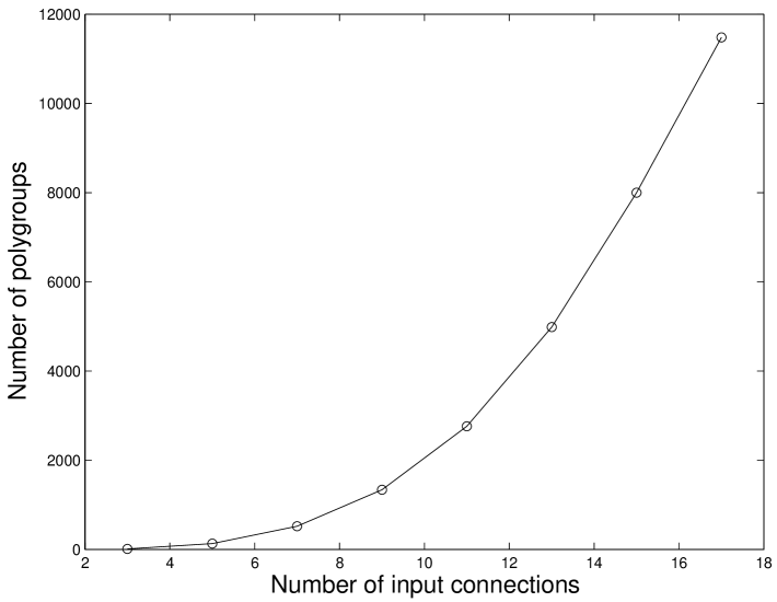
Figure 3: The number of polychronous groups as a function of $m$, the number of input connections to each neuron in the network.

We varied $r$ in the next set of experiments to determine how the number of polychronous groups varies as the the number of nearest neighbors from which input connections are chosen changes. Results are displayed in Figure 4, which shows that the number of polychronous groups decreases rapidly as $r$ is increased. For these runs, $N=100$, $m=5$, $d_{min}=1$, and $d_{max}=5$.

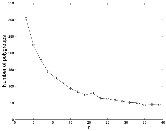
Figure 4: The number of polychronous groups as a function of $r$, the radius of nearest neighbors from which input connections are chosen.

Figure 5 shows what happens as $d_{max}$ is varied. The number of polychronous groups decreases rapidly as $d_{max}$ increases. This is intuitively clear when one considers that as $d_{max}$ increases, the number of possible delays on the connections increases and so the probability of finding pairs of connections with simultaneous arrivals becomes less. For these runs, $N=100$, $m=5$, $r=5$, and $d_{min}=1$.

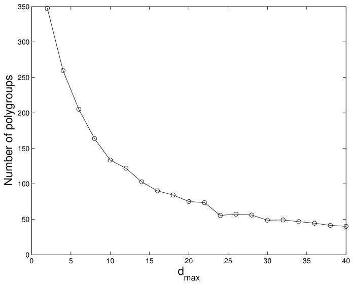
Figure 5: The number of polychronous groups as a function of $d_{max}$, the maximum delay on a connection.

So what do these results tell us about polychronous groups in the human brain? It is estimated that there are $10^{11}$ neurons in the brain, with $m$ in the range of 1000 to 10,000 connections per neuron. Connectivity in the neocortex has been observed to be about 10%, so a good rough estimate of $r$ is 5,000 to 50,000. Experimental measurements of axonal delays have shown that the delay can be as low as 0.1 msec and as high as 40 msec Swadlow (1985) Swadlow (1988) Swadlow (1992). Since the number of polychronous groups scales linearly with the number of neurons, we might expect the number of groups to be roughly on the order of the number of neurons. Of more concern, however, is the scaling relative to the values of $r$, $m$, and $d_{max}$, since these scalings are exponential in nature. Large values of $r$ and $d_{max}$ would tend to lower the total number of polychronous groups, but a large value of $m$ argues for a high number of such groups. The actual result for the human brain cannot even be estimated with the numbers we have so far.

Though the calculation of polychronous groups stretches the capability of current computers, it is possible to define relatively small networks and try to extrapolate measurements on them to networks of a more realistic size. As a baseline we chose a system with the parameters $N=5000$, $m=100$, $r=500$, $d_{min}=1$, and $d_{max}=40$, which took about 12 hours of CPU time to run. For this system there was a total of slightly more than $6.1\times 10^{6}$ polychronous groups. If we were to estimate the number of polychronous groups for this system based solely on the graph in Figure 2, we would expect somewhat over 10,000 groups; the much larger actual total appears to indicate that the exponential growth of the number of polychronous groups due to the increase of $m$ overpowers the decrease brought about by the change due to $r$ and $d_{max}$. This result agrees with that found by Izhikevich in his original paper Izhikevich (2006).

III.2 Results For Two Dimensional Systems

Because of the brain’s layered geometry, it is worthwhile to investigate how dimensionality influences the availability of polychronous groups. Here we address whether or not extending the network to a two-dimensional topology affects the number of polychronous groups. To answer this question both one and two-dimensional networks were constructed using identical parameters. For the two dimensional model, neurons were located on a rectangular grid. The $m$ connections to a given neuron were selected at random within a circle of radius $r$. The parameters for the 1D and 2D networks were selected so that the same number of neurons $N_{r}$ would be included in each sub-region of radius $r$.

The variation of the number of polychronous groups as $N$ changed is shown in Figure 6. Both relationships are clearly linear, though in the two-dimensional case the number of polychronous groups is somewhat less. The slope of the 1D line is approximately 1.0, while the slope for the 2D line is about 0.8. Parameters for these runs were $m=4$, $N_{r}=8$, $d_{min}=1$, and $d_{max}=5$.

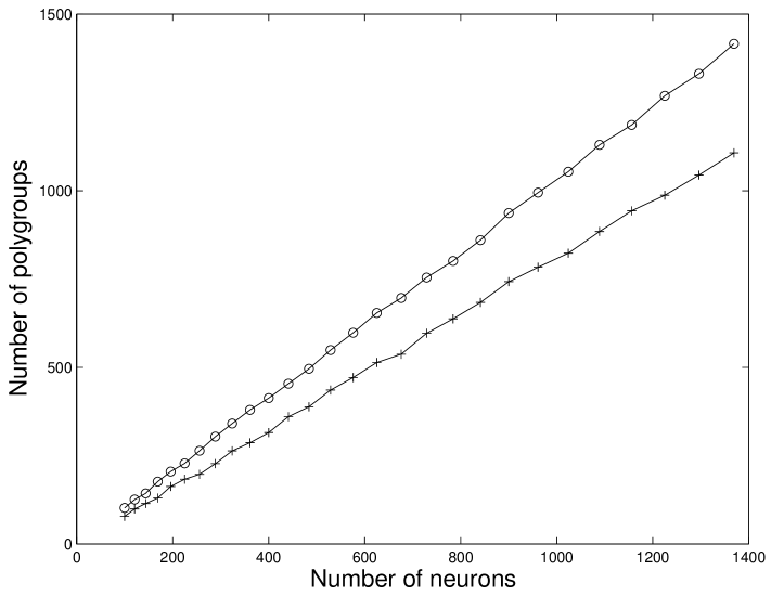
Figure 6: The number of polychronous groups as a function of $N$, the number of neurons in the system, for networks with one- and two-dimensional connectivity. The one-dimensional network graph is marked by small circles, the two-dimensional graph by plus signs.

Figure 7 shows how the number of polychronous groups depends on $m$, the number of input connections. Other parameters were $N=100$, $N_{r}=24$, $d_{min}=1$, and $d_{max}=5$.

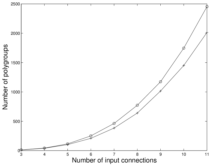
Figure 7: The number of polychronous groups as a function of $m$, the number of input connections per neuron, for networks with one- and two-dimensional connectivity. The one-dimensional network graph is marked by small circles, the two-dimensional graph by plus signs.

Figure 8 shows how the number of polychronous groups depends on $r$, the radius from which input connections are selected. Other parameters were $N=225$, $m=4$, $d_{min}=1$, and $d_{max}=5$.

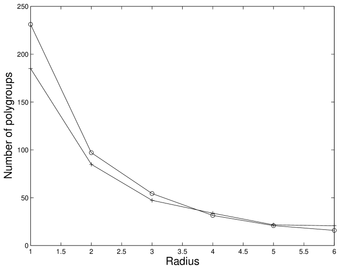
Figure 8: The number of polychronous groups as a function of $r$, the radius from which input connections are selected, for networks with one- and two-dimensional connectivity. The one-dimensional network graph is marked by small circles, the two-dimensional graph by plus signs.

Figure 9 shows how the number of polychronous groups depends on $d_{max}$. Other parameters were $N=100$, $m=4$, $r=2$, and $d_{min}=1$.

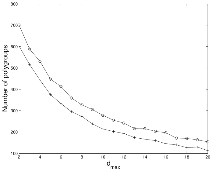
Figure 9: The number of polychronous groups as a function of $d_{max}$, the maximum connection delay, for networks with one- and two-dimensional connectivity. The one-dimensional network graph is marked by small circles, the two-dimensional graph by plus signs.

As can be seen from Figures 6 through 9, the qualitative results for one and two dimensions are similar. The actual number of polychronous groups does vary somewhat with each of the parameters, but not significantly so. The net result of these studies is that changing from one to two dimensions does not change the essential form of the parametric dependencies.

III.3 Choosing Connection Delays Deterministically

In the simulations above the connection delays were chosen randomly within a fixed range. It is a reasonable assumption, however, that in actual networks of neurons the time delay associated with a synaptic connection will be approximately proportional to the distance between the connected neurons. If we use this assumption in our simulations, how does it affect the number of polychronous groups in the network?

Figure 10 shows how the number of polygroups varies with $N$, for both a network with random delays and a network with deterministic delays. Figures 11 and 12 show how the number of polygroups varies with $m$ and $r$, respectively. The essential form of the relationships do not change when using deterministic delays, but the number of polygroups in the networks with deterministic delays is significantly higher than the corresponding networks with randomized delays. It is not immediately clear why the number of groups increases when the delays are proportional to the distance between the connected neurons.

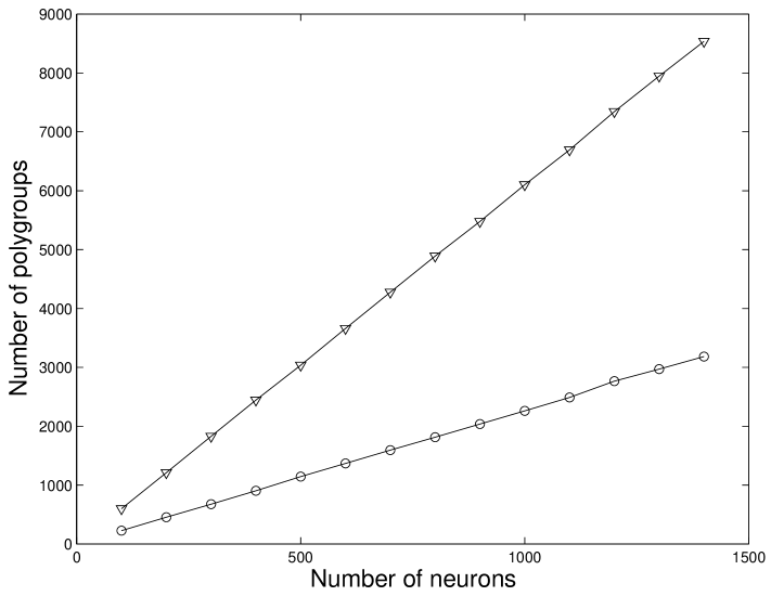
Figure 10: The number of polychronous groups as a function of $N$, the number of neurons in the system, for networks with random vs. deterministic delays. The random network graph is marked by small circles, the deterministic graph by inverted triangles.

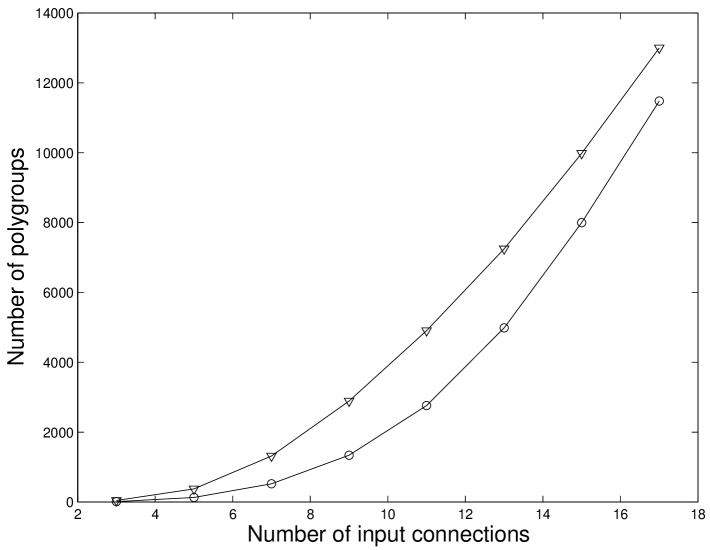
Figure 11: The number of polychronous groups as a function of $m$, the number of input connections per neuron, for networks with random vs. deterministic delays. The random network graph is marked by small circles, the deterministic graph by inverted triangles.

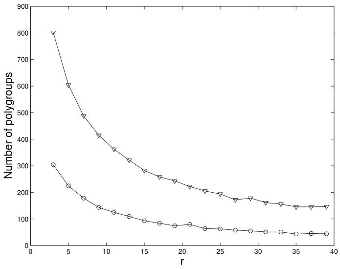
Figure 12: The number of polychronous groups as a function of $r$, the radius from which input connections are selected, for networks with random vs. deterministic delays. The random network graph is marked by small circles, the deterministic graph by inverted triangles.

III.4 How Many Pairs Form Polygroups?

Any given pair of neurons in our neural networks may or may not be capable of stimulating a polychronous group, depending on their synaptic connections and the associated delays, so it is reasonable and interesting to calculate what fraction of the neuron pairs can actually form polygroups. For a neuron with $m$ input connections the number of possible ways that a pair of connections can be chosen is given by

$$\frac{m!}{2!(m-2)!}.$$ (2)

Each pair of input connections has only one timing sequence with which it will trigger the neuron, so this is also the number of ways a particular neuron can be stimulated to fire. For a system with $N$ neurons, the total number of ways for neurons to be stimulated is thus

$$N\frac{m!}{2!(m-2)!}.$$ (3)

Dividing the number of observed polygroups by this number gives us the fraction of pairs that actually created a polygroup. Using the data in Figure 10 for the networks with deterministic delays $(m=5,r=5)$, we find that the fraction of pairs that stimulate polygroups is roughly constant over all $N$, and is equal in this case to approximately 0.6. This may provide a lower bound for more realistic systems where connections are correlated.

IV Computation with polygroups

A polychronous group can be thought of as a sort of automaton; starting with just two firing neurons, an entire chain of neurons is caused to fire over an extended period of time. The group is simply a response to the initial stimulus, and in our perfect simulation world of discrete time and distinct spikes, the response is unvarying. In that sense, then, a polychronous group can be thought of as a monolithic computational element.

When a polygroup is activated, the firing neurons within the group will in most cases have connections to other neurons outside the group. These outside neurons receive only a single spike and thus will not fire. We can envision a "cloud" of such neurons surrounding a polygroup in both space and time.

If two separate polygroups are activated whose firings overlap in time, certain neurons in the surrounding clouds may receive two simultaneous spikes, one from each polygroup, and thus be caused to fire. Furthermore, two or more neurons may be activated in this manner, and their combined action may in turn activate a totally separate polygroup. The net result is that in some cases, the activation of two polygroups can in turn activate a third polygroup.

For a given network, we can label each polygroup with an index $i$ and represent an arbitrary group with the symbol $G_{i}$. To fully specify a polygroup we must know the time at which the group was activated; since the relative times of the activating spikes are fixed, we can choose the time of the first activating spike as the time associated with the polygroup, and thus write $G_{i}^{t}$ to indicate polygroup $i$ activated at time $t$.

If polygroup $G_{1}$ fires at time $t_{1}$ and polygroup $G_{2}$ fires at time $t_{2}$, and if the combined action of these two groups causes another polygroup $G_{3}$ to fire at time $t_{3}$, we can write

$$G_{1}^{t_{1}}+G_{2}^{t_{2}}\rightarrow G_{3}^{t_{3}},$$ (4)

where the symbol $\rightarrow$ is read "activates".

Times are all relative in the system, so any time offset $\tau$ may be added without changing the above relationship:

$$G_{1}^{t_{1}+\tau}+G_{2}^{t_{2}+\tau}\rightarrow G_{3}^{t_{3}+\tau},$$ (5)

If indeed a polychronous group represents a memory in the brain, then equation 4 signifies that certain pairs of memories are capable of stimulating a third memory. Equation 5 shows that the relation of these memories are time invariant. It is interesting, however, that the two stimulating memories must be activated in a fixed time relationship to each other to cause the third memory to activate.

V Summary and conclusions

We have developed a computationally efficient model for the study of polychronous groups, constructed on the principle of including only the essential features required for such groups. An algorithm is included in the model to rapidly identify polygroups in the network. The model was used to computationally investigate properties of polychronous group formation in various network topologies.

Through numerical experiments we found that the number of polygroups in the network depends linearly on the number of neurons, holding all other criteria constant. The number of polygroups decreases asymptotically as the radius of connectivity or the range of time delays increases, but grows exponentially as the number of input connections increases. By testing a larger system we found that the exponential growth of the number of polygroups due to an increase of input connections dominated over the other factors we studied.

We conducted similar experiments comparing one- and two-dimensional networks, and found slight numerical but no qualitative differences in the results. Experiments were then performed in which the transmission delays were chosen to be proportional to the distance between neurons, and when these results were compared with our initial model we discovered that there were no qualitative differences, but that the number of polygroups was much higher for the network with the proportionally chosen delays.

We also introduced the concept of computation using polygroups. In some cases two activated polygroups can cause the stimulation of a third polygroup. This opens up the possibility of polygroups being used as monolithic interacting elements in a neural system. Further work is required to determine the properties of this type of computation.

There are still many open questions regarding polychronous groups, and we have only begun to explore their properties. Further measurements could prove useful, such as determining the distribution of the number of neurons per group under various network topologies. Specific examples that have recently shown a lot of interest are small world and scale free networks Albert and Barabási (2002). Inhibition could also be added to the neural connections, to bring the model more in line with the workings of biological neural systems.

References

- Abeles [1991] M. Abeles. Corticonics. Cambridge University Press, 1991.
- Abeles et al. [1993] M. Abeles, H. Bergman, E. Margalit, and E. Vaadia. Spatiotemporal firing patterns in the frontal cortex of behaving monkeys. Network: Comput. Neural Syst., 6:179–224, 1993.
- Albert and Barabási [2002] Réka Albert and Albert-László Barabási. Statistical mechanics of complex networks. Rev. Mod. Phys., 74(1):47–97, 2002.
- Bienenstock [1995] E. Bienenstock. A model of neocortex. J. Neurophysiol., 70:1629–16384, 1995.
- Claussen [2006] Jens Christian Claussen. Processing of information in synchronously firing chains in networks of neurons. Lecture Notes in Computer Science, 4131:710–717, 2006.
- Doursat and Bienenstock [2006] Rene Doursat and Elie Bienenstock. Neocortical self-structuration as a basis for learning. In 5th International Conference on Development and Learning, 2006.
- Gerstner and Kistler [2002] W. Gerstner and W. Kistler. Spiking Neuron Models. Cambridge University Press, 2002.
- Hosaka et al. [2008] Ryosuke Hosaka, Osamu Araki, and Tohru Ikeguchi. Stdp provides the substrate for igniting synfire chains by spatiotemporal input patterns. Neural Computation, 20:415–435, 2008.
- Izhikevich [2003] E. M. Izhikevich. Simple model of spiking neurons. IEEE Transactions on Neural Networks, 14(6):1569–1572, 2003.
- Izhikevich [2006] E. M. Izhikevich. Polychronization: Computation with spikes. Neural Computation, 18:245–282, 2006.
- Izhikevich et al. [2004] Eugene M. Izhikevich, Joseph A. Gally, and Gerald M. Edelman. Spike-timing dynamics of neuronal groups. Cerebral Cortex, 14:933–944, 2004.
- Rolston et al. [2007] J. D. Rolston, D. A. Wagenaar, and S. M. Potter. Precisely timed spatiotemporal patterns of neural activity in dissociated cortical cultures. Neuroscience, 148:294–303, 2007.
- Swadlow [1985] H. A. Swadlow. Physiological properties of individual cerebral axons studied in vivo for as long as one year. Journal of Neurophysiology, 54:1346–1362, 1985.
- Swadlow [1988] H. A. Swadlow. Efferent neurons and suspected interneurons in binocular visual cortex of the awake rabbit: Receptive fields and binocular properties. Journal of Neurophysiology, 88:1162–1187, 1988.
- Swadlow [1992] H. A. Swadlow. Monitoring the excitability of neocortical efferent neurons to direct activation by extracellular current pulses. Journal of Neurophysiology, 68:605–619, 1992.