Gyrokinetic turbulence: a nonlinear route to dissipation through phase space

Abstract

This paper describes a conceptual framework for understanding kinetic plasma turbulence as a generalized form of energy cascade in phase space. It is emphasized that conversion of turbulent energy into thermodynamic heat is only achievable in the presence of some (however small) degree of collisionality. The smallness of the collision rate is compensated by the emergence of small-scale structure in the velocity space. For gyrokinetic turbulence, a nonlinear perpendicular phase mixing mechanism is identified and described as a turbulent cascade of entropy fluctuations simultaneously occurring at spatial scales smaller than the ion gyroscale and in velocity space. Scaling relations for the resulting fluctuation spectra are derived. An estimate for the collisional cutoff is provided. The importance of adequately modeling and resolving collisions in gyrokinetic simulations is biefly discussed, as well as the relevance of these results to understanding the dissipation-range turbulence in the solar wind and the electrostatic microturbulence in fusion plasmas.

1 Turbulence: the Symptoms and the Cause

What is turbulence? Modulo many definitional and interpretational subtleties [18, 51], turbulence is multiscale disorder: we tend to say that we are dealing with a turbulent system if we have detected (measured, observed, simulated, intuited) chaotic fluctuations of some field(s) over a broad range of scales. In plasmas, these fluctuating fields are the electric and magnetic fields and the distribution function of the particles (either measured directly or accessible partially via its moments: density, flow velocity, temperature). So turbulence is defined as a syndrome [46]: it is identifed by its symptoms. The next logical step is to ask what causes the development of the problem in the first place. The short answer is energy injection: in physical systems, turbulence is stirred up by some source of energy, which is system-specific and can be in the form of direct mechanical forcing (spoon in a tea cup, supernovae in the interstellar medium), boundary conditions (airplane wing), or various instabilities feeding on background equilibrium gradients (tokamak microturbulence, solar convection, magnetorotational turbulence in accretion discs). The fluctuation energy injected into the system is nearly always dissipated into heat. Because the dissipation mechanisms available to the system have to do with its material properties (microphysics) and are usually unrelated to the energy-injection mechanism (macrophysics), there is more often than not a scale separation between the energy-injection, or energy-containing, scale (the outer scale) and the much smaller dissipation scale (the inner scale). In order to dissipate energy, the system has to bridge this gap and one way for this to happen is for the nonlinear interactions to fill the intermediate scale range with fluctuations — giving rise to multiscale disorder, or turbulence (there are, of course, other ways, e.g., shock or current-sheet formation, but we will not consider them here).

The simplest illustration of the argument made above is the case of a Navier-Stokes neutral fluid, whose velocity field $\bi{u}$ satisfies

$$\partial_{t}\bi{u}+\bi{u}\cdot\boldsymbol{\nabla}\bi{u}=-\boldsymbol{\nabla}p+\nu\nabla^{2}\bi{u}+\bi{f},\quad\boldsymbol{\nabla}\cdot\bi{u}=0,$$ (1)

where $p$ is pressure, $\nu$ the molecular viscosity of the fluid, and the body force $\bi{f}$ stands in for the outer-scale energy injection. The kinetic energy of the fluid then satisfies

$${\rmd\over\rmd t}\int{\rmd^{3}\bi{r}\over V}\,{u^{2}\over 2}=\varepsilon-\nu\int{\rmd^{3}\bi{r}\over V}\,|\boldsymbol{\nabla}\bi{u}|^{2},$$ (2)

where $V$ is the system volume and $\varepsilon=(1/V)\int{\rmd^{3}\bi{r}}\,\bi{u}\cdot\bi{f}$ is the injected power per unit volume. In a stationary state, the injection and dissipation terms on the right-hand side of this equation must balance, even though $\varepsilon$ is finite and viscosity is small, or, more precisely, the viscous term in (1) is negligible at the outer scale. The balance is accomplished by transferring kinetic energy to small scales, where the velocity gradients are large, compensating for the viscosity’s smallness. The viscous (inner) scale to which the energy has to travel in order to be dissipated is, on dimensional grounds, $l_{\nu}\sim(\nu^{3}/\varepsilon)^{1/4}\sim L\mathrm{Re}^{-3/4}$, where $L$ is the outer scale and $\mathrm{Re}=u_{\mathrm{rms}}L/\nu$ is the Reynolds number. The system becomes turbulent when $\mathrm{Re}\gg 1$, i.e., $l_{\nu}\ll L$, so fluctuations arise over a broad band of scales.

2 Plasma Turbulence: Entropy, Heating and the Kinetic Cascade

Can this argument be generalized to plasma turbulence? If the plasma is sufficiently collisional, its dynamics is described by a set of fluid equations with diffusive dissipation terms [9]. While things become more complicated than for the Navier–Stokes equation (multiple fields and species, different diffusion coefficients perpendicular and parallel to the magnetic field, interplay between waves and nonlinear interactions), the basic principle remains the same: small-scale spatial structure is generated so that the energy injected at the outer scale can be transferred to the smaller dissipative scales and converted into heat. All this, however, is only valid for fluctuations whose characteristic spatial and temporal scales remain collisional, namely $k_{\parallel}\lambda_{\mathrm{mfp}}\ll 1$ and $\omega\ll\nu_{ii}$, where $k_{\parallel}$ is the typical wavenumber parallel to the magnetic field, $\lambda_{\mathrm{mfp}}$ the particle mean free path and $\nu_{ii}$ the (ion) collision frequency. This requirement is rarely satisfied in real turbulent astrophysical and space plasmas (e.g., in the solar wind, $\lambda_{\mathrm{mfp}}\sim$1 AU) and it is an observational certainty that turbulence exists at collisionless scales [11, 2]. The same is true in fusion plasmas. Thus, plasma turbulence must be understood in the framework of kinetic theory, which evolves the distribution function $f_{s}$ for each species $s$ ($=i,e$):

$${\partial f_{s}\over\partial t}+\bi{v}\cdot\boldsymbol{\nabla}f_{s}+{q_{s}\over m_{s}}\left(\bi{E}+{\bi{v}\times\bi{B}\over c}\right)\cdot{\partial f_{s}\over\partial\bi{v}}=\left({\partial f_{s}\over\partial t}\right)_{\mathrm{c}},$$ (3)

where $q_{s}$ and $m_{s}$ are particle charge and mass, $c$ is the speed of light, the right-hand side of (3) is the collision integral (quadratic in $f$), and $\bi{E}$ and $\bi{B}$ are the electric and magnetic fields, which satisfy Maxwell’s equations:

$$\boldsymbol{\nabla}\cdot\bi{E}=4\pi\sum_{s}q_{s}n_{s},\qquad\qquad\qquad\ \,n_{s}=\int{\rmd^{3}\bi{v}}\,f_{s},$$ (4)

$$\boldsymbol{\nabla}\times\bi{B}-{1\over c}{\partial\bi{E}\over\partial t}={4\pi\over c}\left(\bi{j}+\bi{j}_{\mathrm{ext}}\right),\qquad\bi{j}=\sum_{s}q_{s}\int{\rmd^{3}\bi{v}}\,\bi{v}f_{s},$$ (5)

$${\partial\bi{B}\over\partial t}=-c\boldsymbol{\nabla}\times\bi{E},\qquad\boldsymbol{\nabla}\cdot\bi{B}=0.$$ (6)

In (5), the external current $\bi{j}_{\mathrm{ext}}$ stands in for the outer-scale energy injection.

The energy injected into the plasma must be dissipated and converted into particle heat. It is in fact a rather subtle issue what this exactly means. Multiplying (3) by $m_{s}v^{2}/2$ and integrating, we find that the total particle energy satisfies:

$${\rmd\over\rmd t}\int{\rmd^{3}\bi{r}\over V}\,\sum_{s}\int{\rmd^{3}\bi{v}}\,{m_{s}v^{2}\over 2}\,f_{s}=\int{\rmd^{3}\bi{r}\over V}\,\bi{E}\cdot\bi{j}=\varepsilon-{\rmd\over\rmd t}\int{\rmd^{3}\bi{r}\over V}\,{E^{2}+B^{2}\over 8\pi},$$ (7)

where $\varepsilon=-(1/V)\int{\rmd^{3}\bi{r}}\,\bi{E}\cdot\bi{j}_{\mathrm{ext}}$ is the injected power per unit volume. In deriving the above equation, we used Ampère’s law (5), Faraday’s law (6), and integrated by parts wherever opportune. Equation (7) tells us that, unsurprisingly, the change in particle energy is equal to the work done on the particles ($\int{\rmd^{3}\bi{r}}\,\bi{E}\cdot\bi{j}$) and that the change in the combined energy of the particles and fields is equal to the injected energy. This, however, is not yet a statement about heating in the thermodynamic sense of the term because the energy exchange described by (7) is, in principle, reversible. In order to effect irreversible heating, we must change the entropy of the system and that, in a closed kinetic system, can only be accomplished by collisions. This result is known as Boltzmann’s $H$-theorem [8]: from (3), it is readily obtained [36] that the entropy $S_{s}$ of species $s$ grows according to

$${\rmd S_{s}\over\rmd t}\equiv{d\over dt}\left[-\int{\rmd^{3}\bi{r}\over V}\,\int{\rmd^{3}\bi{v}}\,f_{s}\ln f_{s}\right]=-\int{\rmd^{3}\bi{r}\over V}\,\int{\rmd^{3}\bi{v}}\,\ln f_{s}\left({\partial f_{s}\over\partial t}\right)_{\mathrm{c}}\geq 0.$$ (8)

We would now like to assume that the plasma distribution function can be split into a slowly changing equilibrium part and a fast changing fluctuating part, $f_{s}=F_{0s}+\delta f_{s}$, that the latter is small, and that its smallness is controlled by some parameter $\epsilon\ll 1$. In the next section, we shall specialize to the case of gyrokinetic turbulence, where $\epsilon\sim\omega/\Omega_{i}$, the ratio of the typical fluctuation frequency to the ion cyclotron frequency. As we shall see momentarily, the equilibrium quantities can be assumed to vary on a time scale $\sim(\epsilon^{2}\omega)^{-1}$, much longer than the fluctuation time scale $\omega^{-1}$. We further assume that the collision rate is $\nu_{ii}\sim\omega$, i.e., while the dynamics are not collisionally dominated, collisions are retained on a par with fluctuations. This can be viewed as a convenient ordering prescription on the level of the $\epsilon$ expansion [28] and does not prevent one from considering the collisional ($\nu_{ii}\gg\omega$) and collisionless ($\nu_{ii}\ll\omega$) regimes as subsidiary limits [42]. With these assumptions, (8) implies that the equilibrium distribution is a local Maxwellian for each species [8, 36]: $F_{0s}={n_{0s}}(\pi v_{\mathrm{th}s}^{2})^{-3/2}\exp(-v^{2}/v_{\mathrm{th}s}^{2})$, where $v_{\mathrm{th}s}=(2T_{0s}/m_{s})^{1/2}$ is the thermal speed and $T_{0s}$ the temperature. For simplicity, we shall ignore all spatial gradients of the equilibrium quantities compared to the gradients of the fluctuating ones and also assume that the plasma motions are subsonic, i.e., the Mach number is small, $M=u/v_{\mathrm{th}s}\sim\epsilon\ll 1$.

If we now substitute $f_{s}=F_{0s}+\delta f_{s}$ into (8), use the assumptions explained above, and keep only the lowest-order terms in $\epsilon$, we get

$$T_{0s}\,{\rmd S_{s}\over\rmd t} = {\rmd\over\rmd t}\left[\int{\rmd^{3}\bi{r}\over V}\,\int{\rmd^{3}\bi{v}}\,{m_{s}v^{2}\over 2}\,f_{s}-\int{\rmd^{3}\bi{r}\over V}\,\int{\rmd^{3}\bi{v}}\,{T_{0s}\delta f_{s}^{2}\over 2F_{0s}}\right]$$ (9)

$$= -\int{\rmd^{3}\bi{r}\over V}\,\int{\rmd^{3}\bi{v}}\,{T_{0s}\delta f_{s}\over F_{0s}}\left({\partial\delta f_{s}\over\partial t}\right)_{\mathrm{c}}+\int{\rmd^{3}\bi{v}}\,{m_{s}v^{2}\over 2}\left({\partial F_{0s}\over\partial t}\right)_{\mathrm{c}}.$$

The second term on the right-hand side represents the collisional energy exchange between the Maxwellian equilibria of two species and is equal to $-n_{0s}\nu_{E}^{ss^{\prime}}(T_{0s}-T_{0s^{\prime}})$, where $\nu_{E}^{ss^{\prime}}$ is the appropriate rate of collisions between species $s$ and $s^{\prime}$ [24]. Equation (9) has two key consequences. First, let us average it over times longer than the fluctuation time scale but shorter than the equilibrium-variation time scale, $\omega^{-1}\ll t\ll(\epsilon^{2}\omega)^{-1}$. Then the time derivatives of the fluctuating quantities vanish and, noting that $\int{\rmd^{3}\bi{v}}\,(m_{s}v^{2}/2)F_{0s}=(3/2)n_{0s}T_{0s}$ and $\rmd n_{0s}/\rmd t=0$, we get [28]

$${3\over 2}\,n_{0s}{\rmd T_{0s}\over\rmd t}=-\overline{\int{\rmd^{3}\bi{r}\over V}\,\int{\rmd^{3}\bi{v}}\,{T_{0s}\delta f_{s}\over F_{0s}}\left({\partial\delta f_{s}\over\partial t}\right)_{\mathrm{c}}}-n_{0s}\nu_{E}^{ss^{\prime}}(T_{0s}-T_{0s^{\prime}}),$$ (10)

where the overline denotes the time average. The first term on the right-hand side is positive definite and represents the heating of the equilibrium via collisional dissipation of the fluctuating part of the distribution function — precisely the transfer of the fluctuation energy into heat that is the ultimate imperative of turbulence. Note that (10) is consistent with the ordering assumptions made earlier: the equilibrium evolves on the time scale $\sim(\epsilon^{2}\omega)^{-1}$, as we have ordered $\nu_{ss}\sim\omega$.

The second important consequence of (9) arises if we sum over species and use (7) to express the first term under the time derivative in (9). This gives

$${\rmd\over\rmd t}\int{\rmd^{3}\bi{r}\over V}\,\left[\sum_{s}\int{\rmd^{3}\bi{v}}\,{T_{0s}\delta f_{s}^{2}\over 2F_{0s}}+{E^{2}+B^{2}\over 8\pi}\right]=\varepsilon+\int{\rmd^{3}\bi{r}\over V}\,\sum_{s}\int{\rmd^{3}\bi{v}}\,{T_{0s}\delta f_{s}\over F_{0s}}\left({\partial\delta f_{s}\over\partial t}\right)_{\mathrm{c}}.$$ (11)

The positive definite quantity under the time derivative on the left-hand side, henceforth denoted $W$, will be referred to as generalized energy. Its evolution is determined by the competition (or, in a stationary state, balance) of the externally supplied power $\varepsilon$ and collisional dissipation (the negative-definite term on the right-hand side) — the latter converts the generalized energy into heat according to (10). Thus, we have a conservation law analogous to (2). This suggests a straightforward generalization of the view of fluid turbulence outlined in § 1 to plasma turbulence: its cause and effect is the transfer of the generalized energy injected at the outer scale to scales where the collisional dissipation can convert it to heat.

There is, however, an important novel feature here. If the collision frequency is small, $\nu_{ss}\ll\omega$, the collision term in (11) can only balance the injected power provided the perturbed distribution function develops small-scale structure in velocity space. Since the collision operator is a second-order (diffusion) operator in the velocity space, we may roughly estimate the smallness of this structure by balancing $\omega\sim\nu_{ss}v_{\mathrm{th}s}^{2}\partial^{2}/\partial v^{2}$, so the correlation scale in velocity space is $\delta v/v_{\mathrm{th}s}\sim(\nu_{ss}/\omega)^{1/2}$. As we shall see in § 4, in gyrokinetic turbulence, the emergence of small scales in velocity space is intertwined with a cascade to small scales in physical space. Thus, in the same way as fluid turbulence could be described as the energy cascade, plasma turbulence is a cascade of generalized energy, or a kinetic cascade — this cascade occurs in phase space, reaching towards small scales both in physical space and in velocity space.

If the heating is always ultimately collisional, what then is the status of the collisionless (Landau) damping [35] as a dissipation mechanism for (homogeneous) plasma turbulence? Collisionless damping does not appear explicitly in (11) because what it does is, in fact, redistribute the generalized energy: the energy of electromagnetic fluctuations ($E^{2}+B^{2}$) is converted into entropy fluctuations ($T_{0s}\delta f_{s}^{2}/2F_{0s}$). In order for any actual heating to occur (i.e., for the fluctuation energy to be lost irreversibly), this perturbed entropy has to be transferred through phase space to collisional scales. There are two ways in which this can be accomplished: linear and nonlinear. The first is the well known [23, 47] phase-mixing mechanism associated with the so-called ballistic response in the perturbed distribution function: the linearized kinetic equation (3) has the homogeneous solution $\delta f_{s}\propto\rme^{-\rmi\bi{k}\cdot\bi{v}t}$ [35], for which $\partial\delta f_{s}/\partial v\sim kt\,\delta f_{s}$, i.e., there is a secular growth of the velocity-space derivatives and the collisions become important after a time $t\sim(kv_{\mathrm{th}s})^{-1}(\omega/\nu_{ss})^{1/2}$. In fact, as anticipated in [14] and as we will show in § 4, the linear phase mixing can be superceded by a faster nonlinear mechanism that cascades the perturbed entropy to collisional velocity scales over times $t\sim\omega^{-1}$.

Finally, we note that one can make a plausible argument in favour of an effectively irreversible “collisionless heating” in the sense that the distribution function may become so convoluted in phase space that it is effectively impossible to unscramble it and the entropy of an approppriately defined “coarse-grained” distribution is increased. Discussions of this process and the difference between such effective irreversibility and the exact irreversibility for which collisions are necessary have continued since the birth of quasilinear theory to the present day. Here we only need to emphasize the salient physical fact that until the collsions can act, the negative entropy necessary to compensate for the increase in the coarse-grained entropy is stored in the fluctuations of the perturbed distribution function and that these fluctuations are explicitly present in the overall generalized energy budget (11) — a conservation law that underpins the interpretation of plasma turbulence proposed here.

3 Gyrokinetics and the Many Forms of the Kinetic Cascade

Our treatment so far has not been specific to gyrokinetic turbulence. However, the particular mechanism of kinetic cascade in phase space we intend to discuss in § 4 will be. Thus, we now briefly introduce the gyrokinetic approximation and describe the forms the kinetic cascade from macro to microscales takes in gyrokinetic turbulence.

It is nature’s gift to plasma physicists that magnetized plasma turbulence both in fusion devices and in space appears to consist mostly of fluctuations whose frequencies are much lower than the ion cyclotron frequency, $\omega\ll\Omega_{i}$, even as their spatial scales perpendicular to the magnetic field can be as small as or smaller than the ion gyroscale $\rho_{i}=v_{\mathrm{th}i}/\Omega_{i}$. This low-frequency character of the turbulence is intimately related to the tendency of plasma fluctuations in a dynamically strong magnetic field to be spatially anisotropic, with $k_{\parallel}\ll k_{\perp}$. Let us briefly explain why.

The structure of plasma turbulence is set by the interplay of parallel linear propagation effects (waves, particle streaming) and perpendicular nonlinear decorrelation (turbulent cascade). It is crucial to understand that, while anisotropic, this is an essentially three-dimensional situation. For fluctuations with a given perpendicular correlation length, the parallel correlation length is set by the distance a wave (or streaming particles) can travel during one perpendicular correlation time. A good example of this principle is the Alfvénic MHD turbulence, where it is known as the critical balance [20, 21]. Alfvénic turbulence is the predominant type of turbulence in finite-beta plasmas at scales above the ion gyroscale (the “inertial range”) irrespective of the degree of collisionality — this statement can be proven analytically [41, 42] and there is ample evidence in its favour from measurements in the solar wind [11, 2]. Alfvénic fluctuations have velocities and perturbed magnetic fields $u_{\perp}\sim\delta B_{\perp}/\sqrt{4\pi m_{i}n_{0i}}$ perpendicular to the mean field $\bi{B}_{0}=B_{0}\hat{\bi{z}}$. Their decorrelation rate is $\sim k_{\perp}u_{\perp}$, while the characteristic propagation frequency is $\omega=k_{\parallel}v_{A}$, where $v_{A}=B_{0}/\sqrt{4\pi m_{i}n_{0i}}$. In critical balance, $k_{\parallel}v_{A}\sim k_{\perp}u_{\perp}$, so $k_{\parallel}/k_{\perp}\sim u_{\perp}/v_{A}\ll 1$. If the Alfvénic cascade from the outer scale to the ion gyroscale respects this principle (and there is numerical [12, 37] and observational [25] evidence that it does), the fluctuation frequency at $k_{\perp}\rho_{i}\sim 1$ will still be low compared to the ion cyclotron frequency: $\omega/\Omega_{i}\sim k_{\parallel}v_{A}/\Omega_{i}\sim(k_{\parallel}/k_{\perp})k_{\perp}\rho_{i}/\sqrt{\beta_{i}}\ll 1$ (we assume moderate values of $\beta_{i}$).

The gyrokinetic approximation can now be constructed by using the critical balance explicitly as the ordering prescription: $\epsilon\sim k_{\parallel}/k_{\perp}\sim\omega/\Omega_{i}\sim u_{\perp}/v_{A}\sim q_{s}\varphi/T_{0s}\sim\delta B_{\perp}/B_{0}\sim\delta B_{\parallel}/B_{0}\sim\delta f_{s}/F_{0s}$, where $\varphi$ is the scalar potential. The Vlasov–Maxwell equations (3)–(6) are expanded in $\epsilon$ and averaged over the particle gyromotion [17, 28, 10]. As a result of this procedure, the perturbed distribution function splits into the Boltzmann response and the perturbed distribution of particle gyrocentres: $\delta f_{s}=-q_{s}\varphi F_{0s}/T_{0s}+h_{s}(t,\bi{R}_{s},v_{\perp},v_{\parallel})$, where $\bi{R}_{s}=\bi{r}+\bi{v}_{\perp}\times\hat{\bi{z}}/\Omega_{s}$ is the gyrocentre position. In a uniform magnetic field $\bi{B}_{0}$, the gyrokinetic equation for $h_{s}$ is

$${\partial h_{s}\over\partial t}+v_{\parallel}\,{\partial h_{s}\over\partial z}+{c\over B_{0}}\left\{\langle\chi\rangle_{\bi{R}_{s}},h_{s}\right\}={q_{s}F_{0s}\over T_{0s}}{\partial\langle\chi\rangle_{\bi{R}_{s}}\over\partial t}+\left({\partial h_{s}\over\partial t}\right)_{\mathrm{c}},$$ (12)

where $\chi=\varphi-\bi{v}\cdot\bi{A}/c$, $\bi{B}=B_{0}\hat{\bi{z}}+\delta\bi{B}$, $\delta\bi{B}=\boldsymbol{\nabla}\times\bi{A}$, $\boldsymbol{\nabla}\cdot\bi{A}=0$, and $\langle\cdots\rangle_{\bi{R}_{s}}$ is the gyroangle average at constant $\bi{R}_{s}$. The vector potential $\bi{A}$ is recovered from (5) neglecting the displacement current. The scalar potential $\varphi$ is found from the quasineutrality condition: neglecting $\boldsymbol{\nabla}\cdot\bi{E}$ in (4) and separating the Boltzmann response, we have

$$\sum_{s}{q_{s}^{2}\varphi\over T_{0s}}\,n_{0s}=\sum_{s}q_{s}\int{\rmd^{3}\bi{v}}\,\langle h_{s}\rangle{r},$$ (13)

where $\langle\cdots\rangle{r}$ denotes gyroaveraging at constant $\bi{r}$ (the velocity integral is at constant $\bi{r}$).

Gyrokinetics helps make the problem of kinetic cascade numerically [30, 50] and, in certain limits, analytically [42, 39] tractable because all high-frequency physics ($\omega\geq\Omega_{i}$) is systematically ordered out and the gyroaveraging reduces the phase space from 6D to 5D. However, it is still a fully kinetic system and everything that was said about heating and the kinetic cascade in § 2 remains valid. The generalized energy conservation law (11) for gyrokinetics takes the following form [28, 42]:

$${\rmd W\over\rmd t} = {\rmd\over\rmd t}\int{\rmd^{3}\bi{r}\over V}\,\left[\sum_{s}\left(\int{\rmd^{3}\bi{v}}\,{T_{0s}\langle h_{s}^{2}\rangle{r}\over 2F_{0s}}-{q_{s}^{2}\varphi^{2}n_{0s}\over 2T_{0s}}\right)+{|\delta\bi{B}|^{2}\over 8\pi}\right]$$ (14)

$$= \varepsilon+\sum_{s}\int{\rmd^{3}\bi{v}}\,\int{\rmd^{3}\bi{R}_{s}\over V}\,{T_{0s}h_{s}\over F_{0s}}\left({\partial h_{s}\over\partial t}\right)_{\mathrm{c}}.$$

As we explained in § 2, the generalized energy injected at the outer scale has to be transferred (cascaded) through phase space eventually to reach the collisional scales. If we conjecture that this transfer is local in scale space, we can ask what forms the kinetic cascade takes in several distinct physical regimes separated by the characteristic plasma microscales: the mean free path, the ion and the electron gyroscales. It turns out that in each of the asymptotic limits $k_{\parallel}\lambda_{\mathrm{mfp}}\ll 1$, $k_{\parallel}\lambda_{\mathrm{mfp}}\gg 1$, $k_{\perp}\rho_{i}\ll 1$, $k_{\perp}\rho_{i}\gg 1$, etc., the kinetic cascade splits into several non-energy-exchanging channels corresponding to cascades of distinct plasma fluctuation modes, some of which are familiar from fluid models of plasma turbulence and some are new. As the characteristic scales are crossed ($k_{\parallel}\lambda_{\mathrm{mfp}}\sim 1$, $k_{\perp}\rho_{i}\sim 1$), these channels join together into a single cascade, which then splits again, but in a different way, as another asymptotic limit is reached. All these asymptotic limits are worked out in detail in [42]. Here we briefly summarize their role as a route for the generalized energy to reach the ion gyroscale (at which point interesting things start happening in the phase space).

Let us imagine that energy is injected at scales larger than both the mean free path and the ion gyroradius. As the cascade takes the energy to smaller scales, anisotropy and critical balance are established, so the gyrokinetic approximation applies [29, 27]. In the inertial range ($k_{\perp}\rho_{i}\ll 1$), the energy cascade is split into two main channels: the Alfvénic turbulence ($\delta\bi{B}_{\perp}$, $\bi{u}_{\perp}$), which is described by the Reduced MHD equations [48] regardless of the collisionality [41, 42] and the “compressive” component ($\delta n$, $u_{\parallel}$, $\delta B_{\parallel}$). The Alfvénic cascade is split into two cascades corresponding to the two directions of propagation of the Alfvén waves. While the nonlinear interaction is always between the “$+$” and “$-$” waves, it is of “scatter” type, so no energy is exchanged between the two cascades. The compressive fluctuations are passively mixed by the Alfvén waves, again without energy exchange. In the collisional limit ($k_{\parallel}\lambda_{\mathrm{mfp}}\ll 1$), the compressive cascade is split into three channels: the “$+$” and “$-$” slow waves and the entropy-mode. As $k_{\parallel}\lambda_{\mathrm{mfp}}\sim 1$ is approached, these three are mixed together and remain mixed for $k_{\parallel}\lambda_{\mathrm{mfp}}\gg 1$. Dissipation and collisional heating can occur at this transition because in the fluid limit, the collisional term in (11) can be activated by small deviations of the distribution function from a Maxwellian — the smallness of the collision rate in this case is overcome not by a velocity-space cascade but by the fact that the non-Maxwellian part of the perturbed distribution function is proportional to $k_{\parallel}/\nu_{ii}$. At collisionless scales, the compressive fluctuations experience the Barnes (transit-time) [3, 47] version of Landau damping — as discussed in § 2, this transfers the energy associated with the compressive fluctuations into ion entropy fluctuations.

As the inertial-range cascade transfers energy to scales around $k_{\perp}\rho_{i}\sim 1$, its Alfvénic and compressive components cease to be decoupled from each other and all fluctuations are subject to Landau damping (see [28] for details of linear gyrokinetics). What emerges on the other side of this transition, at $k_{\perp}\rho_{i}\gg 1$, is a cascade of generalized energy again split into two channels: the fluctuations polarized as kinetic Alfvén waves (KAW) (they satisfy fluid-like equations closely related to Electron MHD [31, 42]) and, energetically decoupled from them, the ion entropy fluctuations ($T_{0i}h_{i}^{2}/2F_{0i}$). The latter carry the part of the inertial-range energy that was Landau-damped at the ion gyroscale and, possibly, also in the inertial range (for the compressive fluctuations). How it becomes ion heating is the subject of § 4. The KAW cascade takes the energy to the electron gyroscale, $k_{\perp}\rho_{e}\sim 1$, where it is converted by Landau damping into electron entropy fluctuations ($T_{0e}h_{e}^{2}/2F_{0e}$), eventually giving rise to electron heating in a way analogous to the ion case discussed below.

4 Nonlinear Perpendicular Phase Mixing and the Entropy Cascade

In order to introduce the concept of the phase-space cascade of entropy in the simplest possible setting, we will consider the extreme case where all of the fluctuation energy arriving to the ion gyroscale from the inertial range is converted into entropy fluctuations by Landau damping, i.e., we will neglect the KAW component of the dissipation-range turbulence. Furthermore, we will use the Boltzmann-electrons approximation, which is justified to the lowest order in the mass-ratio expansion as long as we stay above the electron gyroscale, $k_{\perp}\rho_{e}\ll 1$ [45, 42]. These approximations mean that we have $\delta f_{e}=e\varphi F_{0e}/T_{0e}$, i.e., $h_{e}=0$, while $h_{i}$ satisfies the electrostatic version of (12) ($\chi=\varphi$). The resulting system of equations follows from (12) and (13):

$${\partial h_{i}\over\partial t}+v_{\parallel}\,{\partial h_{i}\over\partial z}+{c\over B_{0}}\left\{\langle\varphi\rangle_{\bi{R}_{i}},h_{i}\right\}-\left({\partial h_{i}\over\partial t}\right)_{\mathrm{c}}={\partial\over\partial t}{Ze\langle\varphi\rangle_{\bi{R}_{i}}\over T_{0i}}\,F_{0i},$$ (15)

$$\left(1+{\tau\over Z}\right){Ze\varphi\over T_{0i}}={1\over n_{0i}}\int{\rmd^{3}\bi{v}}\,\langle h_{i}\rangle{r}=\sum{k}\rme^{\rmi\bi{k}\cdot\bi{r}}{1\over n_{0i}}\int{\rmd^{3}\bi{v}}\,J_{0}\left({k_{\perp}v_{\perp}\over\Omega_{i}}\right)h_{i}(\bi{k}),$$ (16)

where $Z=q_{i}/e$, $\tau=T_{0i}/T_{0e}$ and $h_{i}(\bi{k})$ is the Fourier transform of $h_{i}(\bi{R}_{i})$.

As we explained in § 2, in order for the collision term in (15) to become non-negligible, small-scale structure has to be generated in the velocity space with $\delta v/v_{\mathrm{th}i}\sim(\nu_{ii}/\omega)^{1/2}$. One route to such small scales is via the parallel (linear) phase mixing, whose role in plasma turbulence has been well established for some time [23, 34, 33, 52]: the ballistic response $h_{i}\propto\rme^{\rmi k_{\parallel}v_{\parallel}t}$ gives rise to secularly growing gradients $\partial h_{i}/\partial v_{\parallel}\sim k_{\parallel}t\,h_{i}$ and, therefore, small scales in parallel velocities: $\delta v_{\parallel}\sim{1/k_{\parallel}t}$.

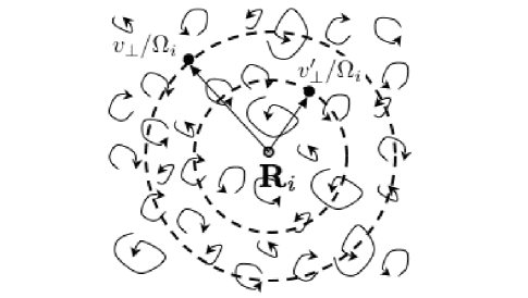
Figure 1: The nonlinear perpendicular phase mixing: the gyrocentre distribution function at a given point $\bi{R}_{i}$ is mixed in a decorrelated way by $\bi{E}\times\bi{B}$ flows gyroaveraged over ion orbits whose radii ($v_{\perp}/\Omega_{i}$ and $v_{\perp}^{\prime}/\Omega_{i}$) differ by more than the flows’ correlation length.

The other, perpendicular, phase mixing mechanism is nonlinear [14, 42]. In (15), the nonlinear term represents mixing of the ion distribution in the gyrocentre space by the gyroaveraged $\bi{E}\times\bi{B}$ flows. Like any random mixing, this produces small scales in $\bi{R}_{i}$. It also produces small scales in $v_{\perp}$ for the following reason. Consider (15) taken at two different values of velocity, $v_{\perp}$ and $v_{\perp}^{\prime}$. Then $h_{i}(\bi{R}_{i},v_{\perp})$ and $h_{i}(\bi{R}_{i},v_{\perp}^{\prime})$ will be spatially mixed by the gyroaveraged $\bi{E}\times\bi{B}$ velocity field given by $\langle\varphi\rangle_{\bi{R}_{i}}(v_{\perp})$ and $\langle\varphi\rangle_{\bi{R}_{i}}(v_{\perp}^{\prime})$, respectively. These gyroaverages come from spatially decorrelated fluctuations of $\varphi$ if the difference between the gyroradii $v_{\perp}/\Omega_{i}$ and $v_{\perp}^{\prime}/\Omega_{i}$ is larger than the perpendicular correlation length $1/k_{\perp}$ of $\varphi$ (figure 1). If this condition is satisfied, $h_{i}(\bi{R}_{i},v_{\perp})$ and $h_{i}(\bi{R}_{i},v_{\perp}^{\prime})$ are mixed by decorrelated fields and are, therefore, themselves decorrelated. Thus, small-scale structure of $\varphi$ in the physical space gives rise to small-scale structure of $h_{i}$ in the velocity space: the correlation scale in the velocity space is

$${\delta v_{\perp}\over v_{\mathrm{th}i}}={1\over\rho_{i}}\left|{v_{\perp}\over\Omega_{i}}-{v_{\perp}^{\prime}\over\Omega_{i}}\right|\sim{1\over k_{\perp}\rho_{i}}\ll 1\quad\mathrm{when}\quad k_{\perp}\rho_{i}\gg 1.$$ (17)

The small-scale structure of $h_{i}$ in the gyrocenter space gives rise to similarly small-scale structure of $\varphi$ in the physical space. Using (16), they can be related as follows. For $k_{\perp}\rho_{i}\gg 1$, the Bessel function in the velocity integral is $J_{0}(k_{\perp}v_{\perp}/\Omega_{i})\simeq(2\Omega_{i}/\pi k_{\perp}v_{\perp})^{1/2}\cos(k_{\perp}v_{\perp}/\Omega_{i}-\pi/4)$, i.e., it oscillates in $v_{\perp}$ with the period $\delta v_{\perp}/v_{\mathrm{th}i}=2\pi/k_{\perp}\rho_{i}$. But, according to (17), this is also the correlation scale of $h_{i}(\bi{k})$ in velocity space. Assuming that the velocity integral accumulates as a random walk and taking into account also the factor of $1/\sqrt{k_{\perp}\rho_{i}}$ coming from the Bessel function, we have

$${Ze\varphi(\bi{k})\over T_{0i}}\sim{v_{\mathrm{th}i}^{3}\over n_{0i}}{1\over\sqrt{k_{\perp}\rho_{i}}}\left({\delta v_{\perp}\over v_{\mathrm{th}i}}\right)^{1/2}h_{i}(\bi{k})\sim{v_{\mathrm{th}i}^{3}\over n_{0i}}{h_{i}(\bi{k})\over k_{\perp}\rho_{i}}.$$ (18)

The gyroaveraged potential is then $Ze\langle\varphi\rangle_{\bi{R}_{i}}(\bi{k})/T_{0i}=ZeJ_{0}(k_{\perp}v_{\perp}/\Omega_{i})\varphi(\bi{k})/T_{0i}\sim(v_{\mathrm{th}i}^{3}/n_{0i})h_{i}(\bi{k})/(k_{\perp}\rho_{i})^{3/2}$, and so the perpendicular mixing of the particle distribution is a fully nonlinear process.

This process can be understood as a local (in scale) ion entropy cascade and a Kolmogorov-style scaling theory can be constructed for it. Recall that the gyrokinetic equation (15) has a conservation law given by (14) with $h_{e}=0$ and $\delta\bi{B}=0$. In view of (18), $Z^{2}e^{2}\varphi^{2}n_{0i}/2T_{0i}\ll\int{\rmd^{3}\bi{v}}\,T_{0i}h_{i}^{2}/2F_{0i}$, so the entropy of the perturbed ion distribution is conserved individually. This is, in fact, obvious also from (15): again using (18), the inhomogeneous term on the right-hand side is negligible for $k_{\perp}\rho_{i}\gg 1$ and $\int d^{3}\bi{R}_{i}\,h_{i}^{2}$ is clearly a conserved quantity but for collisions. Denoting by $\varphi_{\lambda}$ and $h_{i\lambda}$ the characteristic fluctuation amplitudes at some perpendicular scale $\lambda\ll\rho_{i}$ and by $\tau_{\lambda}$ the corresponding cascade time, we may write (cf. footnotes 2 and 8)

$${m_{i}v_{\mathrm{th}i}^{8}\over n_{0i}}{h_{i\lambda}^{2}\over\tau_{\lambda}}\sim\varepsilon,\qquad\tau_{\lambda}\sim\left({\rho_{i}\over\lambda}\right)^{1/2}{\lambda^{2}\over c\varphi_{\lambda}/B_{0}}\sim{\rho_{i}^{1/2}\lambda^{1/2}n_{0i}\over v_{\mathrm{th}i}^{4}h_{i\lambda}},$$ (19)

where we used (18) to get $c\varphi_{\lambda}/B_{0}\sim v_{\mathrm{th}i}^{4}h_{i\lambda}\lambda/n_{0i}$. Combining these relations, we find

$$h_{i\lambda}\sim{n_{0i}\over v_{\mathrm{th}i}^{3}}{\rho_{i}^{1/6}\lambda^{1/6}\over l_{0}^{1/3}},\qquad{Ze\varphi_{\lambda}\over T_{0i}}\sim{\lambda^{7/6}\over\rho_{i}^{5/6}l_{0}^{1/3}},\qquad\tau_{\lambda}\sim{l_{0}^{1/3}\rho_{i}^{1/3}\lambda^{1/3}\over v_{\mathrm{th}i}},$$ (20)

where $l_{0}=m_{i}n_{0i}v_{\mathrm{th}i}^{3}/\varepsilon$. These scalings correspond to a $k_{\perp}^{-4/3}$ spectrum of $h_{i}$ and a $k_{\perp}^{-10/3}$ spectrum of $\varphi$. Encouragingly, these predictions seem to be corroborated by numerical simulations of electrostatic gyrokinetic turbulence in two spatial dimensions [50].

Now let us revisit the question of parallel phase mixing. In our discussion of the perpendicular cascade so far, we have ignored the presence of the parallel propagation (particle streaming) term in (15). In a formally 2D situation, i.e., when $\omega\sim\tau_{\lambda}^{-1}\gg k_{\parallel}v_{\parallel}$, this is, of course, allowed and the perpendicular scalings derived above should hold. However, it is more likely that the parallel scale of the fluctuations will adjust to their perpendicular scale according to the critical balance principle explained in § 3: $l_{\parallel\lambda}$ for the fluctuations with perpendicular scale $\lambda$ will be such that particles can stream across the distance $l_{\parallel\lambda}$ in one nonlinear decorrelation time $\tau_{\lambda}$. Using (20), this implies $l_{\parallel\lambda}\sim v_{\mathrm{th}i}\tau_{\lambda}\sim l_{0}^{1/3}\rho_{i}^{1/3}\lambda^{1/3}$ (cf. footnote 8). As we explained at the beginning of this section, the typical parallel correlation scale in velocity space produced by the parallel phase mixing is $\delta v_{\parallel}\sim 1/k_{\parallel}t$. Therefore, after one perpendicular cascade time, no appreciable refinement of the parallel velocity-space structure is achieved: $\delta v_{\parallel}/v_{\mathrm{th}i}\sim l_{\parallel\lambda}/v_{\mathrm{th}i}\tau_{\lambda}\sim 1$. In contrast, in $v_{\perp}$, one cascade time is enough for the entire cascade down to the collisional cutoff (to be calculated in § 5) to be set up. Thus, the linear parallel phase mixing is much less efficient than the nonlinear perpendicular one.

5 Conclusion: Dissipation Achieved

Let us now come back to the original motivation for the above developments: the necessity to understand how the distribution function is brought to collisional scales in the velocity space. We have seen that this is done by transferring the energy injected at the outer scale down to the ion and electron gyroscales via a multichannel cascade of generalized energy through phase space. Below the ion gyroscale, the phase-space nature of the cascade becomes particularly manifest as the ion distribution function simultaneously develops small scales in the gyrocentre and velocity space via a nonlinear perpendicular phase mixing process. We have described this process as a Kolmogorov-like turbulent cascade enabled by a constant flux of ion entropy and derived scaling relations for the fluctuations of the distribution function and the electric potential.

Using these scalings (20), let us now estimate the collisional cutoff in phase space. As we explained in § 2, the collisional scale is reached if the velocity-space correlation scale is $\delta v/v_{\mathrm{th}i}\sim(\nu_{ii}/\omega)^{1/2}$. Using (17) and estimating $\omega\sim\tau_{\lambda}^{-1}$, we get

$${\delta v_{\perp c}\over v_{\mathrm{th}i}}\sim{1\over k_{\perp c}\rho_{i}}\sim\left(\nu_{ii}\tau_{\rho_{i}}\right)^{3/5}\sim{l_{0}^{1/5}\rho_{i}^{2/5}\over\lambda_{\mathrm{mfp}}^{3/5}},$$ (21)

where $l_{0}=m_{i}n_{0i}v_{\mathrm{th}i}^{3}/\varepsilon$ and $\tau_{\rho_{i}}\sim(m_{i}n_{0i}\rho_{i}^{2}/\varepsilon)^{1/3}$ is the fluctuation time scale at $k_{\perp}\rho_{i}\sim 1$. This formula is perhaps our most consequential result for numerical applications: it tells us what it means to have a well-resolved gyrokinetic simulation of plasma turbulence and shows that the resolution requirements in the gyrocentre and velocity spaces are fundamentally linked. In this context, it is clear that adequate modeling of collisions [1, 5] and controlled velocity-space resolution [4] are imperative for gyrokinetic simulations.

No matter how small the collisional cutoff (21) is, all of the energy channelled into the sub-gyroscale entropy cascade will reach this cutoff in finite time — roughly the nonlinear interaction scale $\tau_{\rho_{i}}$ evaluated at the ion gyroscale. Since the process is nonlinear, this time is amplitude dependent. If the principle of critical balance (§ 3) holds at the ion gyroscale, $\tau_{\rho_{i}}$ should be roughly equal to the linear parallel propagation time scale at $k_{\perp}\rho_{i}\sim 1$. Importantly, the time to reach the collisional cutoff does not depend on the collision rate — just like in hydrodynamic turbulence (§ 1), the time to reach the viscous scale is the turnover time at the outer scale, independent of viscosity.

Another important conclusion is that the dissipation range ($k_{\perp}\rho_{i}>1$), even in the absence of kinetic Alfvén waves, is filled with electrostatic fluctuations due to the ion entropy cascade. This is a purely kinetic effect invisible in any fluid models. In fusion plasmas, this may be relevant for identifying the nature of electrostatic fluctuations found between the ion and electron gyroscales. In space physics, the great variability of the observed spectra in the dissipation range [44] might be speculatively attributed to varying proportions of energy contained in the entropy and kinetic-Alfvén-wave cascades [42].

These results are only the first glimpse of what one finds if one adopts the view of plasma turbulence as a kinetic cascade in phase space. We believe that further studies conducted in this vein, both numerical [30, 50] and analytical [42, 39], will unveil much new physics and many new and tantalizing questions.

References

References

- [1] Abel I G et al2008 Phys. Plasmas submitted
- [2] Bale S D et al2005 Phys. Rev. Lett.94 215002
- [3] Barnes A 1966 Phys. Fluids 9 1483
- [4] Barnes M A 2008 Ph. D. Thesis (University of Maryland)
- [5] Barnes M A et al2008 Phys. Plasmas submitted
- [6] Bilato R and Brambilla M 2004 Plasma Phys. Control. Fusion46 1455
- [7] Boldyrev S A 2006 Phys. Rev. Lett.96 115002
- [8] Boltzmann L 1872 Sitsungsber. Akad. Wiss. Wien 66 275 [English translation: in Kinetic Theory 2 ed S G Brush (Oxford: Pergamon, 1966) 88]
- [9] Braginskii S I 1965 Rev. Plasma Phys. 1 205
- [10] Brizard A J and Hahm T S 2007 Rev. Mod. Phys.79 421
- [11] Bruno R and Carbone V 2005 Living Rev. Solar Phys. 2 4
- [12] Cho J and Vishniac E T 2000 Astrophys. J. 539 273
- [13] Cowley S C, Kulsrud R M and Sudan R 1991 Phys. Fluids B 3 2767
- [14] Dorland W and Hammett G W 1993 Phys. Fluids B 5 812
- [15] Dorland W et al2000 Phys. Rev. Lett.85 5579
- [16] Fowler T K 1968 Adv. Plasma Phys. 1 201
- [17] Frieman E A and Chen L 1982 Phys. Fluids 25 502
- [18] Frisch U 1995 Turbulence (Cambridge: Cambridge University Press)
- [19] Galtier S et al, 2000 J. Plasma Phys. 63 447
- [20] Goldreich P and Sridhar S 1995 Astrophys. J. 438 763
- [21] Goldreich P and Sridhar S 1997 Astrophys. J. 485 680
- [22] Hallatschek K 2004 Phys. Rev. Lett.93 125001
- [23] Hammett G W, Dorland W and Perkins F W 1991 Phys. Fluids B 4 2052
- [24] Helander P and Sigmar D J 2002 Collisional Transport in Magnetized Plasmas (Cambridge: Cambridge University Press)
- [25] Horbury T S, Forman M A and Oughton S 2008 Phys. Rev. Lett.submitted [Preprint arXiv:0807.3713]
- [26] Horton W 1999 Rev. Mod. Phys.71 735
- [27] Howes G G 2008 Phys. Plasmas 15 055904
- [28] Howes G G et al2006 Astrophys. J. 651 590
- [29] Howes G G et al2008 J. Geophys. Res. 113 A05103
- [30] Howes G G et al2008 Phys. Rev. Lett.100 065004
- [31] Kingsep A S, Chukbar K V and Yankov V V 1990 Rev. Plasma Phys. 16 243
- [32] Kolmogorov A N 1941 Dokl. Akad. Nauk SSSR 30 299 [English translation: Proc Roy. Soc. London A 434 9 (1991)]
- [33] Krommes J A 1999 Phys. Plasmas 6 1477
- [34] Krommes J A and Hu G 1994 Phys. Plasmas 1 3211
- [35] Landau L 1946 J. Phys. USSR 10 25
- [36] Longmire C L 1963 Elementary Plasma Physics (New York: Interscience)
- [37] Maron J and Goldreich P 2001 Astrophys. J. 554 1175
- [38] Obukhov A M 1941 Izv. Akad. Nauk SSSR Ser. Geogr. Geofiz. 5 453
- [39] Plunk G G 2008 Ph. D. Thesis (UCLA)
- [40] Richardson L F 1922 Weather Prediction by Numerical Process (Cambridge: Cambridge University Press)
- [41] Schekochihin A A, Cowley S C and Dorland W 2007 Plasma Phys. Control. Fusion49 A195
- [42] Schekochihin A A et al2007 Astrophys. J. Suppl. submitted [Preprint arXiv:0704.0044]
- [43] Scott B D 2007 Phys. Plasmas submitted [Preprint arXiv:0710.4899]
- [44] Smith C W et al2006 Astrophys. J. 645 L85
- [45] Snyder P B and Hammett G W 2001 Phys. Plasmas 8 3199
- [46] Stewart R W 1969 Turbulence film directed by the National Committee for Fluid Mechanics Films, produced by EDC, Inc. [URL: http://web.mit.edu/fluids/www/Shapiro/ncfmf.html]
- [47] Stix T H 1992 Waves in Plasmas (New York: AIP)
- [48] Strauss H R 1976 Phys. Fluids 19 134
- [49] Sugama H et al1996 Phys. Plasmas 3 2379
- [50] Tatsuno T et al2008 Phys. Rev. Lett.submitted
- [51] Tsinober A 2001 An Informal Introduction to Turbulence (Dordrecht: Kluwer)
- [52] Watanabe T-H and Sugama H 2004 Phys. Plasmas 11 1476