Magnetization Relaxation and Collective Spin Excitations in Correlated Double–Exchange Ferromagnets

Abstract

We study spin relaxation and dynamics of collective spin excitations in correlated double–exchange ferromagnets. For this, we introduce an expansion of the Green’s functions equations of motion that treats non–perturbativerly all correlations between a given number of spin and charge excitations and becomes exact within a sub–space of states. Our method treats relaxation beyond Fermi’s Golden Rule while recovering previous variational results for the spin–wave dispersion. We find that the momentum dependence of the spin–wave dephasing rate changes qualitatively due to the on–site Coulomb interaction, in a way that resembles experiment, and depends on its interplay with the magnetic exchange interaction and itinerant spin lifetime. We show that the collective spin relaxation and its dependence on the carrier concentration depends sensitively on three–body correlations between a spin excitation and a Fermi sea electron and hole. The above spin dynamics can be controlled via the itinerant carrier population.

I Introduction

Long–range ferromagnetic order mediated by interactions between itinerant and localized spins is established in many different materials.nagaev ; tokura ; tokura1 ; III-V The manganese oxides $\rm{R_{1-x}A_{x}MnO_{3}}$ (R=La,Pr,Nd,Sm,$\dots$ and $\rm{A=Ca,Ba,Sr,Pd,}\dots$) are one prominent example. tokura The magnetic and transport properties of such itinerant magnetic systems are intimately related and, unlike in other ferromagnets, can potentially be controlled by tuning parameters like the itinerant carrier density.

Learning how to control magnetization dynamics and relaxation is important for spintronics applications. tokura1 ; wolf ; LLG-rev One of the challenges facing future magnetic devices and memories concerns their speed, which is governed by the dynamics of the collective spin. For small deviations from equilibrium, the dynamical magnetic properties are determined by the spin susceptibility. LLG-rev ; heinr ; mitchell ; sinova ; halp Within the Random Phase approximation (RPA), heinr ; furukawa ; RPA ; nagaev-HP ; golosov ; sun ; papanico which gives the spin susceptibility to $O(1/S)$ ($S$ is the local spin magnitude), magnetization relaxation arises from the interplay between the dephasing of the itinerant carrier spin and the magnetic exchange interaction. mitchell ; sinova ; halp ; chovan Spin relaxation also arises from inelastic scattering processes, such as magnon scattering with charge excitations. kats ; golosov ; chubukov Experimental probes of such effects include neutron scattering, ferromagnetic resonance, and ultrafast magneto–optical pump–probe spectroscopy. bigot-05 ; kampen ; kimel-anis ; tolk ; lupke ; kimel-rev ; wang-rev ; shah ; chovan The interpretation of such experiments requires the development of many–body theories of spin dynamics and relaxation.

Our goal in this paper is to develop a theory that describes the local spin Green’s function

$$\ll S^{+}_{-{\bf Q}}\gg=-i\theta(t)<[S^{+}_{-{\bf Q}}(t),S_{\bf Q}^{-}(0)]>,$$ (1)

which determines the transverse spin susceptibility. In the above we introduced the collective spin operators ${\bf S}^{n}_{{\bf q}}=1/\sqrt{N}\sum_{j}{\bf S}^{n}_{j}\rm{e}^{-i{\bf q}\cdot{\bf R}_{j}}$, $n$=x,y,z, where ${\bf S}_{j}$ describe spins localized on $N$ lattice sites at positions ${\bf R}_{j}$. $S^{\pm}=S^{x}\pm iS^{y}$ are the spin raising/lowering operators and $\langle\cdots\rangle$ denotes the grand canonical ensemble average. We consider a model Hamiltonian that accounts for the most important features common in a wide range of different itinerant ferromagnets, $H=K+H_{\rm{exch}}+H_{\rm{AF}}+H_{U}$. $K=\sum_{\bf k\sigma}\varepsilon_{\bf k}c_{\bf k\sigma}^{\dagger}c_{\bf k\sigma}$ describes a band of itinerant carriers, which in the manganites arises from the Mn d–states with $e_{g}$ symmetry. $c^{\dagger}_{\bf k\sigma}$ creates an electron with momentum ${\bf k}$, spin $\sigma$, and energy $\varepsilon_{\bf k}$. To simplify the calculation of correlation effects common in many different physical systems, we consider a one–band model of $n=1-x$ itinerant electrons per Mn atom that hop between nearest–neighbour ltice sites. The electron concentration is described by the filling factor $n=N_{e}/N$, where $N_{e}$ is the total number of electrons, which varies from 0 to 1. $\varepsilon_{\bf k}=-t\gamma_{\bf k}$, where $\gamma_{{\bf k}}=2\sum_{i=1}^{d}\rm{cos}(k_{i}a)$. $d$ is the system dimensionality and $a$ the lattice constant ($a=\hbar=1$ from now on). In the manganites, 0.5$\leq n\leq$0.8 in the metallic ferromagnetic regime of interest here. Our calculation can be extended to include the bandstructure of individual materials.

In momentum space, the magnetic exchange interaction between the local and itinerant spins is given by

$$H_{\rm{exch}} = -\frac{J}{2\sqrt{N}}\sum_{\bf k,q\sigma}\sigma S_{\bf q}^{z}c_{\bf k-q\sigma}^{\dagger}c_{\bf k\sigma}$$ (2)

$$-\frac{J}{2\sqrt{N}}\sum_{\bf k,q}\Big{(}S_{\bf q}^{-}c_{\bf k-q\uparrow}^{\dagger}c_{\bf k\downarrow}+\rm{H.c}\Big{)}$$

where $\sigma=\pm 1$. In the manganites, Eq.(2) describes the Hund’s rule onsite interaction between the $e_{g}$ carrier spin and the $S=3/2$ local magnetic moment of the three electrons in the tightly bound $t_{2g}$ Mn orbitals. $J\sim 2\rm{eV}$ and $0.2\rm{eV}\leq t\leq 0.5\rm{eV}$ are typical values quoted in the literature, which give $4\leq J/t\leq 10$.dagotto The Hamiltonian $K+H_{\rm{exch}}$ defines the simple double–exchange model.de ; dagotto

Here we add to the above minimal double exchange Hamiltonian two ubiquitous interactions;

$$H_{U}=\frac{U}{N}\sum_{\bf kk^{\prime}q}c_{{\bf k+q}\uparrow}^{\dagger}c_{\bf k^{\prime}-q\downarrow}^{\dagger}c_{\bf k^{\prime}\downarrow}c_{\bf k\uparrow},$$ (3)

is the on–site (Hubbard) Coulomb repulsion. The Coulomb energy $U\sim 3.5-8\rm{eV}$ is the largest energy scale in the manganites.dagotto This Hubbard interaction is generally hard to treat and its effects on the spin dynamics have received less attention.golosov ; sun ; kapet2

$$H_{\rm{AF}} = J_{\rm{AF}}\sum_{\bf k}\gamma_{\bf k}S_{\bf k}^{z}S_{-\bf k}^{z}$$ (4)

$$+\frac{J_{\rm{AF}}}{2}\sum_{k}\gamma_{\bf k}(S_{\bf k}^{+}S_{-\bf k}^{-}+S_{\bf k}^{-}S_{-\bf k}^{+})$$

is the direct super–exchange anti–ferromagnetic interaction between the nearest–neighbor local spins. $J_{\rm{AF}}\sim$0.01t is weak in the manganites.dagotto

Given the large values of $J/t$ in most systems of interest, many theories start from the strong coupling limit ($J\rightarrow\infty$) of the above Hamiltonian. In this limit, the itinerant carriers can hop on a site only if their spin is parallel to the local spin there. The kinetic energy is reduced when all spins are parallel (double exchange mechanism de ), which favors the fully polarized half–metallic state $|F\rangle$. In the classical limit, $S\rightarrow\infty$, the problem can be mapped to an effective nearest neighbor Heisenberg model with ferromagnetic interactions. The lowest order ($O(1/S)$) quantum corrections are described by the RPA, which for strong couplings gives a dispersion that again coincides with that of the nearest neighbor Heisenberg ferromagnet. furukawa We may therefore assess the importance of correlations and quantum fluctuations beyond $O(1/S)$ by fitting the Heisenberg dispersion to the experimental result and looking for deviations.

For electron concentrations $n\geq 0.7$, initial measurements found nearest neighbor Heisenberg model spin dynamics.sw-exp-1 However, later experiments reported deviations that increase strongly for $n\leq$0.7. soft-exp-1 ; soft-exp-2 ; soft-exp-3 ; soft-exp-4 ; endoh ; soft-2D-1 ; soft-2D-2 ; ye The Heisenberg model with nearest neigbor interactions, $J_{1}$, misses a pronounced softening near the Brillouin zone boundary. This softening is accompanied by a strong increase in the spin–wave damping as we approach the zone boundary. The experimental dispersion could be fitted by adding a fourth–nearest–neighbour ferromagnetic exchange interaction, $J_{4}$, to $J_{1}$ while keeping $J_{3}$=$J_{2}$=0.ye

The above experimental observations reveal a new spin dynamics and nonlocal correlations that are not captured by the strong coupling limit of the double exchange model (which favors local correlations). Several scenarios have been put forward. The proposed mechanisms involve, among others, magnon scattering with orbital degrees of freedom,khal ; endoh Fermi sea pairs,kapet1 ; kapet2 or phonons soft-exp-2 ; endoh ; edwards , disorder effects,disord bandstructure effects,solovyev Hubbard interactions golosov and correlations kapet2 , and the energetic overlap between spin–wave modes and the Stoner continuum.kaplan The observed pronounced dependence of the spin–wave dynamics on the carrier concentration puts stringent conditions on the theory. Ye et.al. ye argued that none of the mechanisms proposed so far can fully account for all aspects of this spin dynamics.

The purpose of this paper is two–fold. First, we study the momentum dependence of the spin–wave dephasing rate, with the focus on the role of correlations between the spin and charge excitations and on their interplay with the itinerant spin dephasing. We demonstrate that both the magnitude and the momentum dependence of the spin relaxation rates depend sensitively on the carrier concentration and on correlations due to both $J$ and $U$. We show that the on–site Coulomb repulsion $U$ changes the momentum dependence of the spin–wave dephasing rate in a qualitative way that resembles the experimental results. We also show that our results depend on the interplay of $U$ with the itinerant carrier spin lifetime, which is finite in some systems due to interactions not included in our Hamiltonian. heinr ; mitchell We compare with the 1/S expansion and other approximations and find that three–body correlations between spin and electron–hole pair excitations play an important role. Finally, we show that the magnetization relaxation can be controlled by tuning the carrier density. We obtain changes in the spin relaxation with $n$ that correlate with corresponding changes in the spin–wave softening and non–Heisenberg behavior.

Second, we develop and test a general method for describing spin dynamics. For this we use a truncation scheme of the infinite hierarchy of Green’s function equations of motion based on an expansion in terms of correlations. Our scheme treats the full dynamics induced by the correlations between a given number of elementary excitations. Here we describe all correlations between a local or carrier spin excitation and an electron–hole Fermi sea pair and obtain the exact solution within the sub–space of states with up to one Fermi sea excitation. Similar to Refs.[kapet1, ; kapet2, ], our method becomes exact in the limits of one electron ($N_{e}$=1, $n$=1/$N$), half filling ($N_{e}$=$N$, $n$=1), and in the atomic limit ($t$=0 for any $n$). It interpolates between the weak and strong coupling limits and agrees with exact diagonalization results for the spin–wave dispersion.exact Finally, it retains its variational nature in the limit of zero relaxation rates, which provides a rigorous bound for the spin–wave softening and ferromagnetic phase boundary. Our approach, used before in the context of the Hubbard Hamiltonian, igar ; rucken is in the same spirit as the projection and factorization scheme of Ref.[perakis, ], used to calculate the ultrafast nonlinear optical response of systems with a strongly correlated ground state, and the correlation expansion of Ref.[corr-exp, ]. It may be extended to study spin correlations in non–equilibrium systems chovan ; shah and the magnetization dynamics of (III,Mn)V semiconductors.unpubl

The rest of this paper is organized as follows. In Section II we discuss the Green’s function truncation scheme and derive a closed system of equations of motion that determine the spin Green’s function. In Section III we obtain the spin self–energy and separate the RPA contribution from the contributions of correlations due to $J$ and $U$. In Section IV we discuss our numerical results for the spin–wave dephasing rate and dispersion and compare different approximations. In Section IV.1 we consider the minimal double exchange model with $U$=$J_{AF}$=0, while in Section IV.2 we study how $U$ and $J_{AF}$ change the picture. We end with our conclusions in Section V.

II Truncation of Green’s Function Hierarchy

In this section we obtain the equations of motion that determine the Green’s function Eq.(1) and the spin susceptibility. The many–body interactions $H_{exch}$ and $H_{U}$ introduce an infinite hierarchy of coupled equations of motion that involve higher Green’s functions of the form

$$\ll A\gg=-i\theta(t)<[A(t),S_{\bf Q}^{-}(0)]>,$$ (5)

where $A(t)=\exp{(iHt)}A\exp{(-iHt)}$ are many–body Heisenberg operators. To truncate this hierarchy, we approximate the higher Green’s functions by systematically adding correlations among any given number of elementary excitations. To lowest order, the RPA describes uncorrelated quasi–particles. At the next level, we include all correlations between any two elementary excitations, which determine the inelastic dephasing rate.

Ref.[igar, ] used a three–body scattering theory to calculate the electron Green’s function of the Hubbard Hamiltonian. In one dimension, the results obtained this way were in excellent agreement with the exact Bethe ansatz solution.igar ; rucken In Ref.[perakis, ], a similar method was used to calculate the density matrix that describes the coherent ultrafast nonlinear optical dynamics of the Quantum Hall system. Refs.[fes-1, ; fes-2, ; fes-3, ] calculated the Fermi Edge Singularity in doped semiconductor quantum wells using an analogous approach. In this paper, we establish the correspondence with a factorization scheme of higher Green’s functions. For simplicity we restrict to zero temperature, where Eq.(5) involves the ground state average value.

In the case of ferromagnetic exchange interaction as in the manganites, the fully polarized state

$$|F\rangle=\prod_{\nu}\,c^{{\dagger}}_{\nu\uparrow}|0\rangle\bigotimes|S,S,\cdots\rangle,$$ (6)

is an exact eigenstate of the many-body Hamiltonian $H$. In Eq.(6), $|0\rangle$ is the vacuum state and $|S,S,\cdots\rangle$ describes local spins with $S_{z}=S$ on all lattice sites. From now on, the indices $\mu,\nu,\cdots$ denote states occupied in $|F\rangle$, while $\alpha,\beta,\cdots$ denote empty states. In the parameter range of interest here, $|F\rangle$ is the ground state. kapet1 ; kapet2 Using the properties $H|F\rangle=0$ (we choose the eigenvalue of $|F\rangle$ as the zero of energy) and $\langle F|S^{-}_{{\bf Q}}=0$, both of which stem from the fact that $|F\rangle$ is the state with maximum spin, we obtain from Eq.(5)

$$\ll A\gg=-i\theta(t)<F|Ae^{-iHt}S_{\bf Q}^{-}|F>.$$ (7)

The Green’s function $\ll A\gg$ is then given by the amplitude of the time–evolved state $S_{\bf Q}^{-}|F>$. The hierarchy of Green’s function equations of motion is equivalent to solving the time–dependent Schrödinger equation. However, Green’s functions also treat dephasing and relaxation, and can describe phenomenologically the effects of coupling to degrees of freedom not included in the Hamiltonian $H$ by introducing phenomenological damping rates. The coupling of $\ll A\gg$ to higher Green’s functions is determined by the states $HA|F\rangle$. Truncation of the equations of motion hierarchy can be achieved by expanding $HA|F\rangle$ in a truncated basis, which gives the exact solution within a subspace of states.

We start with the equation of motion for the spin Green’s function Eq.(1), obtained after straightforward algebra by using Eq.(7) and the properties of $|F\rangle$:

$$\left(i\partial_{t}-\frac{Jn}{2}-\omega^{\rm{AF}}_{\bf Q}\right)\ll S_{\bf-Q}^{\dagger}\gg$$

$$=2S\delta(t)-\frac{JS}{\sqrt{N}}\sum_{\nu}\ll c_{\nu\uparrow}^{\dagger}c_{\bf\nu+Q\downarrow}\gg$$

$$+\frac{J}{2N}\sum_{\alpha\nu}\ll S_{\bf\alpha-\nu-Q}^{\dagger}c_{\bf\nu\uparrow}^{\dagger}c_{\bf\alpha\uparrow}\gg,$$ (8)

and

$$\omega^{\rm{AF}}_{\bf Q}=2J_{\rm{AF}}S(\gamma_{\bf Q}-\gamma_{\bf 0})$$ (9)

is the spin–wave energy due to $H_{\rm{AF}}$. The same result can alternatively be obtained by decomposing the Green’s functions contributing to $\ll[S^{+}_{{\bf-Q}},H]\gg$ into correlated and uncorrelated parts after using the identity

$$\ll S^{n}_{{\bf q}}c^{\dagger}_{{\bf k-Q-q}\sigma}c_{{\bf k}\sigma^{\prime}}\gg$$

$$=\langle c^{\dagger}_{{\bf k-Q-q}\sigma}c_{{\bf k}\sigma^{\prime}}\rangle\ll S^{n}_{{\bf q}}\gg$$

$$+\langle S^{n}_{{\bf q}}\rangle\ll c^{\dagger}_{{\bf k-Q-q}\sigma}c_{{\bf k}\sigma^{\prime}}\gg$$

$$+\ll\Delta S^{n}_{{\bf q}}\Delta[c^{\dagger}_{{\bf k-Q-q}\sigma}c_{{\bf k}\sigma^{\prime}}]\gg,$$ (10)

where $S^{n}$ are the components of the local spin and $\Delta A=A-\langle A\rangle$ describes the quantum fluctuations of $A$. The Green’s function $\ll\Delta S^{n}\Delta[c^{\dagger}_{\sigma}c_{\sigma^{\prime}}]\gg$ is the correlated part of $\ll S^{n}c^{\dagger}_{\sigma}c_{\sigma^{\prime}}\gg$.

The Green’s function $\ll c_{\nu\uparrow}^{\dagger}c_{\bf\nu+Q\downarrow}\gg$ describes the itinerant carrier spin dynamics and satisfies the following equation of motion, obtained after straightforward algebra by using Eq.(7) and the properties of $|F\rangle$:

$$(i\partial_{t}-\varepsilon_{\bf\nu+Q}+\varepsilon_{\bf\nu}-JS-nU)\ll c_{\nu\uparrow}^{\dagger}c_{\bf\nu+Q\downarrow}\gg=$$

$$-\frac{J}{2\sqrt{N}}\ll S_{\bf-Q}^{\dagger}\gg-\frac{U}{N}\sum_{\mu}\ll c_{\mu\uparrow}^{\dagger}c_{\bf\mu+Q\downarrow}\gg$$

$$-\frac{J}{2\sqrt{N}}\sum_{\bf\alpha}\ll S_{\bf\alpha-\nu-Q}^{\dagger}c_{\bf\nu\uparrow}^{\dagger}c_{\bf\alpha\uparrow}\gg$$

$$-\frac{U}{N}\sum_{\alpha\mu}\ll c_{\bf\mu\uparrow}^{\dagger}c_{\bf Q+\mu+\nu-\alpha\downarrow}c_{\bf\nu\uparrow}^{\dagger}c_{\bf\alpha\uparrow}\gg_{c}.$$ (11)

where we defined the correlated part of the four–particle Green’s function as

$$\ll c^{\dagger}_{1}c_{2}c^{\dagger}_{3}c_{4}\gg_{c}=\ll c^{\dagger}_{1}c_{2}c^{\dagger}_{3}c_{4}\gg$$

$$-\langle c^{\dagger}_{1}c_{2}\rangle\ll c^{\dagger}_{3}c_{4}\gg-\langle c^{\dagger}_{3}c_{4}\rangle\ll c^{\dagger}_{1}c_{2}\gg$$

$$-\langle c_{2}c^{\dagger}_{3}\rangle\ll c^{\dagger}_{1}c_{4}\gg+\langle c^{\dagger}_{1}c_{4}\rangle\ll c^{\dagger}_{3}c_{2}\gg.$$ (12)

Alternatively, Eq.(11) can be derived by using Eq.(10) to decompose the Green’s function $\ll[c_{\nu\uparrow}^{\dagger}c_{\bf\nu+Q\downarrow},H]\gg$. The first line on the right hand side (rhs) of Eqs.(II) and (11) gives the RPA result, which neglects all non–factorizable (correlated) contributions to Eqs.(10) and (12) (Tyablikov approximation tyablikov ).

Eqs.(II) and (11) reduce the calculation of the spin Green’s function to that of two higher Green’s functions, $\ll\Delta S^{+}\Delta[c_{\bf\uparrow}^{\dagger}c_{\bf\uparrow}]\gg$ and $\ll c_{\bf\uparrow}^{\dagger}c_{\bf\downarrow}c_{\bf\uparrow}^{\dagger}c_{\bf\uparrow}\gg_{c}$. In a system with a general ground state, two additional Green’s functions, $\ll\Delta S^{z}\Delta[c_{\uparrow}^{\dagger}c_{\downarrow}]\gg$ and $\ll\Delta S^{+}\Delta[c_{\downarrow}^{\dagger}c_{\downarrow}]\gg$, also couple and describe ground state correlations. unpubl However, these vanish here since, for the groud state Eq.(6), $\Delta S^{z}|F\rangle$=0 and $c_{\downarrow}^{\dagger}c_{\downarrow}|F\rangle$=0. For the same reason, $\ll c_{\bf\mu\uparrow}^{\dagger}c_{\downarrow}c_{\bf\nu\uparrow}^{\dagger}c_{\bf\alpha\uparrow}\gg=\ll c_{\bf\mu\uparrow}^{\dagger}c_{\downarrow}c_{\bf\nu\uparrow}^{\dagger}c_{\bf\alpha\uparrow}\gg_{c}$ and $\ll S^{+}c_{\bf\nu\uparrow}^{\dagger}c_{\bf\alpha\uparrow}\gg=\ll\Delta S^{+}\Delta[c_{\bf\nu\uparrow}^{\dagger}c_{\bf\alpha\uparrow}]\gg$. Also, from Eq.(7) we see that $\ll A\gg=0$ for any $A$ such that $\langle F|A=0$.

The Green’s function $\ll S^{+}c_{\bf\nu\uparrow}^{\dagger}c_{\bf\alpha\uparrow}\gg$ describes the correlations between a magnon, an electron, and a Fermi sea hole (three–body correlations), while the Green’s function $\ll c_{\bf\mu\uparrow}^{\dagger}c_{\bf Q+\mu+\nu-\alpha\downarrow}c_{\bf\nu\uparrow}^{\dagger}c_{\bf\alpha\uparrow}\gg_{c}$ describes the correlations between two Fermi sea holes and two electrons of opposite spin. These two Green’s functions are obtained from the following equations of motion, derived from Eq.(7) after using the properties of $|F\rangle$:

$$\left(i\partial_{t}-\varepsilon_{\bf\alpha}+\varepsilon_{\bf\nu}-\frac{Jn}{2}-\omega^{\rm{AF}}_{{\bf Q}+\nu-\alpha}\right)\ll S_{\bf\alpha-\nu-Q}^{\dagger}c_{\bf\nu\uparrow}^{\dagger}c_{\bf\alpha\uparrow}\gg$$

$$=\frac{J}{2N}\ll S_{\bf-Q}^{\dagger}\gg-\frac{JS}{\sqrt{N}}\ll c_{\bf\nu\uparrow}^{\dagger}c_{\bf\nu+Q\downarrow}\gg$$

$$+\frac{J}{2N}\sum_{\bf\beta}\ll S_{\bf\beta-\nu-Q}^{\dagger}c_{\bf\nu\uparrow}^{\dagger}c_{\bf\beta\uparrow}\gg$$

$$-\frac{J}{2N}\sum_{\bf\mu}\ll S_{\bf\alpha-\mu-Q}^{\dagger}c_{\bf\mu\uparrow}^{\dagger}c_{\bf\alpha\uparrow}\gg$$

$$-\frac{JS}{\sqrt{N}}\sum_{\bf\mu}\ll c_{\bf\mu\uparrow}^{\dagger}c_{\bf Q+\mu+\nu-\alpha\downarrow}c_{\bf\nu\uparrow}^{\dagger}c_{\bf\alpha\uparrow}\gg_{c}$$ (13)

and

$$\left(i\partial_{t}-\varepsilon_{\bf Q+\mu+\nu-\alpha}-\varepsilon_{\bf\alpha}+\varepsilon_{\bf\nu}+\varepsilon_{\bf\mu}-JS-nU\right)\times$$

$$\ll c_{\bf\mu\uparrow}^{\dagger}c_{\bf Q+\mu+\nu-\alpha\downarrow}c_{\bf\nu\uparrow}^{\dagger}c_{\bf\alpha\uparrow}\gg_{c}$$

$$=\frac{J}{2\sqrt{N}}\left[\ll S_{\bf\alpha-\mu-Q}^{\dagger}c_{\bf\mu\uparrow}^{\dagger}c_{\bf\alpha\uparrow}\gg-\ll S_{\bf\alpha-\nu-Q}^{\dagger}c_{\bf\nu\uparrow}^{\dagger}c_{\bf\alpha\uparrow}\gg\right]$$

$$+\frac{U}{N}\left[\ll c_{\bf\mu\uparrow}^{\dagger}c_{\bf\mu+Q\downarrow}\gg_{c}-\ll c_{\bf\nu\uparrow}^{\dagger}c_{\bf\nu+Q\downarrow}\gg\right]$$

$$-\frac{U}{N}\left[\sum_{\mu^{\prime}}\ll c_{{\bf\mu^{\prime}}\uparrow}^{\dagger}c_{\bf Q+\mu^{\prime}+\nu-\alpha\downarrow}c_{\bf\nu\uparrow}^{\dagger}c_{\bf\alpha\uparrow}\gg_{c}\right.$$

$$\left.+\sum_{\nu^{\prime}}\ll c_{{\bf\mu}\uparrow}^{\dagger}c_{\bf Q+\mu+\nu^{\prime}-\alpha\downarrow}c_{\bf\nu^{\prime}\uparrow}^{\dagger}c_{\bf\alpha\uparrow}\gg_{c}\right.$$

$$\left.-\sum_{\alpha^{\prime}}\ll c_{{\bf\mu}\uparrow}^{\dagger}c_{\bf Q+\mu+\nu-\alpha^{\prime}\downarrow}c_{\bf\nu\uparrow}^{\dagger}c_{\bf\alpha^{\prime}\uparrow}\gg_{c}\right].$$ (14)

Eqs.(II) and (II) describe vertex corrections to the carrier–spin interaction. The first line on the rhs of Eq.(II) gives the Born approximation. The second and third lines describe vertex corrections due to the multiple scattering of the localized spin with the Fermi sea pair electron (second line) and hole (third line). Neglecting the third line corresponds to assuming a non–interacting (static fes-1 ) Fermi sea, equivalent to summing only the electron–magnon ladder diagrams (two–body ladder approximation).igar By also including the hole multiple scattering processes (third line), we treat exactly all correlations between local spin, electron, and hole, a three–body problem. The last line on the rhs of Eq.(II) comes from correlations between two electrons and two holes, described by Eq.(II). We note that $U$ introduces new correlations among all four of the above particles, described by the last four lines on the rhs of Eq.(II).

To obtain the above closed system of equations, we neglected the coupling to Green’s functions of the form $\ll Ac^{\dagger}_{\nu\uparrow}c_{\mu\uparrow}^{\dagger}c_{\alpha\uparrow}c_{\beta\uparrow}\gg$, where $A=S^{+}$ or $c^{\dagger}_{\nu^{\prime}\uparrow}c_{\downarrow}$. These neglected Green’s functions describe multi–particle correlations between two Fermi sea pairs and a local spin or carrier spin–flip excitation, which contribute to higher order in 1/S. Alternatively, we can arrive at the same result by decomposing the Green’s functions $\ll S^{+}c^{\dagger}_{\uparrow}c_{\uparrow}^{\dagger}c_{\uparrow}c_{\uparrow}\gg$ and $\ll c^{\dagger}_{\uparrow}c_{\downarrow}c^{\dagger}_{\uparrow}c_{\uparrow}^{\dagger}c_{\uparrow}c_{\uparrow}\gg$ into uncorrelated and correlated parts, by separating out all possible factorizable contributions similar to Ref.[corr-exp, ], and neglecting the fully correlated contributions that describe correlations among three excitations. This correlation expansion neglects the contribution of states with two or more Fermi sea pair excitation and corresponds to an exact calculation of the Green’s functions within the sub–space of states with up to one Fermi sea pair. As discussed e.g. in Refs.[igar, ; rucken, ] and implied by Eq.(7), in the limit $\gamma$,$\Gamma$$\rightarrow$0 the exact calculation of the Green’s function within a given subspace it equivalent to the variational calculation of the spin–wave energy using a variational wavefunction that is a linear combination of the states that span the subspace (obtained in Refs.[kapet1, ; kapet2, ] for the problem at hand). One could include multipair correlations, e.g., by extending the approach of Refs. [linden, ,fes-2, , fes-3, ].

III Spin Self Energy

The spin self energy can be calculated by solving the equations of motion derived above by Fourier transformation. Eq.(II) gives

$$\ll S_{\bf-Q}^{\dagger}\gg_{\omega}=\frac{2S}{\omega-\omega^{\rm{AF}}_{\bf Q}-\Sigma(\omega,{\bf Q})},$$ (15)

where $\Sigma(\omega,{\bf Q})$ is the self energy. Defining for convenience

$$X_{\nu}(\omega,{\bf Q})=\frac{\ll c_{\nu\uparrow}^{\dagger}c_{\bf\nu+Q\downarrow}\gg_{\omega}}{\ll S_{\bf-Q}^{+}\gg_{\omega}},$$ (16)

$$G_{\alpha\nu}(\omega,{\bf Q})=\frac{\ll S_{\bf\alpha-\nu-Q}^{\dagger}c_{\bf\nu\uparrow}^{\dagger}c_{\bf\alpha\uparrow}\gg_{\omega}}{\ll S_{\bf-Q}^{+}\gg_{\omega}},$$ (17)

$$\Phi^{\alpha}_{\mu\nu}(\omega,{\bf Q})=\frac{\ll c_{\mu\uparrow}^{\dagger}c_{\bf Q+\mu+\nu-\alpha\downarrow}c_{\nu\uparrow}^{\dagger}c_{\alpha\uparrow}\gg_{\omega}}{\ll S_{\bf-Q}^{+}\gg_{\omega}}$$ (18)

and substituting into Eqs.(II), (11), (II), and (II) we express the self energy in the form

$$\Sigma(\omega,{\bf Q})=\frac{Jn}{2}-\frac{\Delta}{\sqrt{N}}\sum_{\nu}X_{\nu}+\frac{J}{2N}\sum_{\alpha\nu}G_{\alpha\nu},$$ (19)

where $\Delta=JS$ is the magnetic energy. We calculate $\Sigma$ non–perturbatively in the interactions and $1/S$ by solving the following coupled equations for $X$, $G$, and $\Phi$:

$$\left(nU+\Delta+\varepsilon_{\bf\nu+Q}-\varepsilon_{\nu}-\omega\right)X_{\nu}-\frac{U}{N}\sum_{\mu}X_{\mu}$$

$$=\frac{J}{2\sqrt{N}}\left(1+\sum_{\alpha}G_{\alpha\nu}\right)+\frac{U}{N}\sum_{\alpha\mu}\Phi_{\mu\nu}^{\alpha},$$ (20)

$$\left(\omega+\varepsilon_{\nu}-\varepsilon_{\alpha}-\frac{Jn}{2}-\omega^{AF}_{\bf Q-\alpha+\nu}+i\gamma\right)G_{\alpha\nu}$$

$$=\frac{J}{2N}\left(1+\sum_{\beta}G_{\beta\nu}-\sum_{\mu}G_{\alpha\mu}\right)$$

$$-\frac{\Delta}{\sqrt{N}}\left(X_{\nu}+\sum_{\mu}\Phi_{\mu\nu}^{\alpha}\right),$$ (21)

where $\gamma\rightarrow 0$, and

$$\left(nU+\Delta+\varepsilon_{\alpha}+\varepsilon_{\bf Q+\mu+\nu-\alpha}-\varepsilon_{\mu}-\varepsilon_{\nu}-\omega\right)\Phi_{\mu\nu}^{\alpha}$$

$$=\frac{J}{2\sqrt{N}}\left(G_{\alpha\nu}-G_{\alpha\mu}\right)+\frac{U}{N}\left(X_{\nu}-X_{\mu}\right)$$

$$+\frac{U}{N}\left(\sum_{\mu^{\prime}}\Phi_{\mu^{\prime}\nu}^{\alpha}+\sum_{\nu^{\prime}}\Phi_{\mu\nu^{\prime}}^{\alpha}-\sum_{\beta}\Phi_{\mu\nu}^{\beta}\right).$$ (22)

First we consider the RPA self energy, obtained by setting $G=\Phi=0$ in the above equations. We can then solve Eq.(20) analytically after noting that its solution has the form

$$X^{\rm{RPA}}_{\nu}(\omega,{\bf Q})=\frac{\chi^{\rm{RPA}}(\omega,{\bf Q})}{nU+\Delta+\varepsilon_{\bf\nu+Q}-\varepsilon_{\nu}-\omega}.$$ (23)

Substituting the above expression into Eq.(20) we obtain

$$\chi^{\rm{RPA}}(\omega,{\bf Q})=\frac{J}{2\sqrt{N}}\frac{1}{1-\frac{U}{N}\sum_{\mu}\frac{1}{nU+\Delta+\varepsilon_{\bf\mu+Q}-\varepsilon_{\mu}-\omega}}.$$ (24)

which gives after some straightforward algebra

$$X^{\rm{RPA}}_{\nu}(\omega,{\bf Q})=\frac{J}{2\sqrt{N}}\frac{1}{\Delta+U_{{\bf\nu Q}}+\varepsilon_{\bf\nu+Q}-\varepsilon_{\nu}-\omega},$$ (25)

where we introduced the Coulomb–induced energy

$$U_{{\bf\nu Q}}=\frac{U}{N}\sum_{\mu}\frac{\varepsilon_{\bf\mu+Q}-\varepsilon_{\mu}-\varepsilon_{\bf\nu+Q}+\varepsilon_{\nu}}{nU+\Delta-i\Gamma+\varepsilon_{\bf\mu+Q}-\varepsilon_{\mu}-\omega}.$$ (26)

Substituting Eq.(25) into Eq.(19) after setting $G=0$ we obtain the RPA self energy

$$\Sigma^{\rm{RPA}}(\omega,{\bf Q})=\frac{J}{2N}\sum_{\nu}\frac{U_{{\bf\nu Q}}+\varepsilon_{\bf\nu+Q}-\varepsilon_{\nu}-\omega}{\Delta-i\Gamma+U_{{\bf\nu Q}}+\varepsilon_{\bf\nu+Q}-\varepsilon_{\nu}-\omega}.$$ (27)

Following Ref.[heinr, ], in the above equations we added a phenomenological relaxation rate $\Gamma$ that describes the itinerant spin lifetime due to interactions not included in our Hamiltonian $H$. This result can alternatively be obtained by substituting $\Delta$ by $\Delta-i\Gamma$, as derived with the Lindblad semigroup method in Ref.[chovan, ]. In the intrinsic system described by the Hamiltonian $H$, $\Gamma$$\rightarrow$0.

We now turn to the self–energy due to the correlations. By formally solving Eq.(20) for $X_{\nu}$ and substituting into Eq.(19), we separate the self–energy into RPA and correlated contributions, $\Sigma(\omega,{\bf Q})=\Sigma^{\rm{RPA}}(\omega,{\bf Q})+\Sigma^{\rm{corr}}(\omega,{\bf Q})$. After some algebra we obtain that $\Sigma^{\rm{corr}}(\omega,{\bf Q})=\Sigma^{\rm{corr}}_{J}(\omega,{\bf Q})+\Sigma^{\rm{corr}}_{U}(\omega,{\bf Q})$.

$$\Sigma^{\rm{corr}}_{J}=\frac{J}{2N}\sum_{\alpha\nu}G_{\alpha\nu}\frac{U_{{\bf\nu Q}}+\varepsilon_{\bf\nu+Q}-\varepsilon_{\nu}-\omega}{\Delta-i\Gamma+U_{{\bf\nu Q}}+\varepsilon_{\bf\nu+Q}-\varepsilon_{\nu}-\omega}$$ (28)

is the contribution of the Fermi sea–magnon correlations due to $J$, described by the Green’s function $G$, Eq.(21).

$$\Sigma^{\rm{corr}}_{U}=-\frac{U}{N^{3/2}}\sum_{\alpha\nu\mu}\Phi^{\alpha}_{\mu\nu}\frac{\Delta-i\Gamma}{\Delta-i\Gamma+U_{{\bf\nu Q}}+\varepsilon_{\bf\nu+Q}-\varepsilon_{\nu}-\omega}$$ (29)

is the contribution of the Fermi sea pair–carrier spin–flip four–particle correlations described by $\Phi$ and discussed in Ref.[kapet2, ]. This latter contribution vanishes for $U$=0.

IV Numerical results

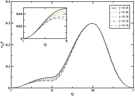
Figure 1: (Color online) Spin–wave dispersion for different values of $\gamma/t$ for $J=8t,n=0.6,U=J_{AF}=\Gamma=0$. Inset: Dispersion along the $\Gamma\to X$ direction.

In this section we present our numerical results for the spin–wave dispersion, which we obtain by solving self–consistently the equation

$$\omega_{{\bf Q}}=\omega^{\rm{AF}}_{{\bf Q}}+\rm{Re}\Sigma(\omega_{{\bf Q}},{\bf Q}),$$ (30)

and the spin–wave dephasing rate $\Gamma_{{\bf Q}}$, determined by $\rm{Im}\Sigma(\omega_{{\bf Q}},{\bf Q})$. We focus on the inelastic contribution to the dephasing rate, due to the scattering between spin and charge excitations: $\Gamma_{{\bf Q}}=\Gamma^{J}_{{\bf Q}}+\Gamma^{U}_{{\bf Q}}$, where

$$\Gamma^{J}_{{\bf Q}}=-\rm{Im}\Sigma^{\rm{corr}}_{J}(\omega_{{\bf Q}},{\bf Q})$$ (31)

is the contribution due to the magnon–Fermi sea pair correlations described by $G$, Eq.(28), and

$$\Gamma^{U}_{{\bf Q}}=-\rm{Im}\Sigma^{\rm{corr}}_{U}(\omega_{{\bf Q}},{\bf Q})$$ (32)

is the contribution due to the carrier spin flip–Fermi sea pair correlations described by $\Phi$, Eq.(22). An additional elastic contribution to the spin–wave lifetime can come from the imaginary part of the RPA self energy, which however vanishes in the limit $\Gamma\rightarrow 0$ due to the finite carrier spin–flip excitation energy. Within the RPA, spin–wave dephasing can only arise from the interplay between the magnetic exchange interaction and carrier spin dephasing via external couplings.mitchell ; heinr

Below we study the momentum dependence of $\Gamma_{{\bf Q}}$ along different directions in the Brillouin zone. We focus, in particular, on the directions $\Gamma$–$X$, $\Gamma$–$M$, and $X$–$M$, where $\Gamma=(0,0),X=(\pi,0)$, and $M=(\pi,\pi)$. Our calculations were performed on a 20$\times$20 square lattice, which as shown in Refs.[kapet1, ] and [kapet2, ] gives good convergence to the thermodynamic limit. Any small size effects are washed out when the relaxation rate $\gamma$ in Eq.(21) exceeds the energy spacing.

IV.1 Minimal double–exchange model

First we consider the simple double exchange Hamiltonian and set $U=J_{AF}=\Gamma=0$. Fig.1 shows the spin–wave dispersion $\omega_{{\bf Q}}$ as function of the damping rate $\gamma$ in Eq.(21). With decreasing $\gamma$, our results converge to the spin–wave dispersion obtained variationally in Ref.[kapet1, ] and the $\gamma\rightarrow 0$ limit. Similar to the experiment,ye our calculation can then be fitted to the dispersion of the Heisenberg Hamiltonian with first– and fourth–nearest–neighbor spin interactions $J_{1}$ and $J_{4}$.kapet2 For intermediate concentrations, our calculation gives a pronounced spin–wave softening at the X point, described by $J_{4}$, as compared to both the RPA and to the fit to the nearest neighbor Heisenberg dispersion. The effects of a finite $\gamma$ are most pronounced along the direction $\Gamma\to X$: with increasing $\gamma$, the time evolution described by the Green’s function $G$, which determines the spin–wave softening, is suppressed and thus the dispersion starts to approach the RPA ($G=0$) result. From now on we fix $\gamma=0.2t$, which as can be seen in Fig.1 is close to the $\gamma\rightarrow 0$ limit.

Fig.2 demonstrates the important role of correlations due to spin–charge interactions on both the spin–wave dispersion and dephasing rate. The spin–wave energies and lifetimes differ markedly depending on the approximation used to treat the correlations. The latter determine the differences from the RPA, which describes non–interacting spin–waves ($G=\Phi$=0). The RPA grossly underestimates the softening and does not give any spin damping in the limit $\Gamma\rightarrow 0$.

By neglecting the Green’s function $\Phi$, we obtain spin–wave energies closer to the RPA (see Fig.2(a)). As seen in Fig.2(b), this approximation, which only treats the scattering of local spins with the Fermi sea, gives a very small damping rate. On the other hand, the non–variational $O(1/S^{2})$ approximation discussed in Refs.[golosov, ; chubukov, ], which treats magnon–Fermi sea scattering within the Born approximation and Fermi’s golden rule, strongly overestimates the softening, while at the same time predicting only a small damping rate (see Fig.2).

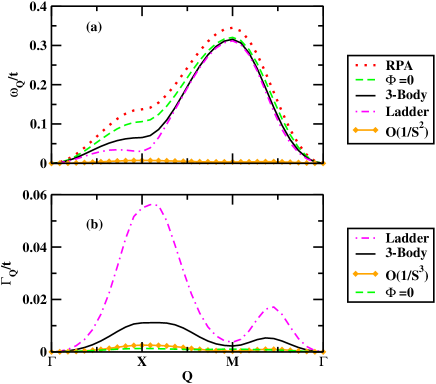
Figure 2: (Color online) Comparison of the different approximations for treating the correlations for $U$=0. (a) Spin–wave dispersion, (b) Inelastic spin–wave dephasing rate. $n=0.6,J=8t,\gamma=0.2t,U=J_{\rm{AF}}=\Gamma=0$.

By adding to the $O(1/S^{2})$ result the effects of the multiple scattering of the magnon with the Fermi sea pair electron, while still neglecting the magnon–Fermi sea hole interactions, we obtain a non–variational two–body approximation of the vertex corrections equivalent to summing the magnon–electron ladder diagrams.igar As can be seen in Fig.2, this ladder approximation gives very large softening and damping, much larger than the predictions of the full calculation (which is variational in the limit $\gamma,\Gamma$$\rightarrow$0 considered here). The latter treats, in addition to the magnon–electron interactions, the multiple scattering of the Fermi sea pair hole with the magnon. The large differences between the ladder and full calculation results demonstrate the importance of three–body correlations between magnon, electron, and hole in the parameter regime of interest in the manganites. We conclude based on Fig.2 that all correlations between spin, electron, and hole must be treated on an equal basis. The variational nature of our full calculation of the spin–wave energies in the limit $\gamma,\Gamma$$\rightarrow$0 has the advantage of providing a rigorous limit of the magntitude of the softening, unlike for the ladder or 1/S expansion results.

Fig.3 shows the behavior of $\omega_{{\bf Q}}$ and $\Gamma_{{\bf Q}}$ for different interactions $J$. With increasing interaction strength, the spin–wave energies increase and the ferromagnetic phase becomes more stable. This hardening with $J$ is accompanied by a corresponding increase in the spin–wave lifetime. The above changes are stronger along the $\Gamma$–$X$ direction, where the non–Heisenberg behavior and softening are pronounced, and depend nonlinearly on $J$/$t$. The overall momentum dependence, however, remains the same for all $J$.

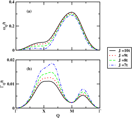
Figure 3: (Color online) Dependence of the spin dynamics on the interaction strength $J$. Spin–wave dispersion (a) and dephasing rate (b). $n=0.6,\gamma=0.2t,\Gamma=U=J_{AF}=0$.

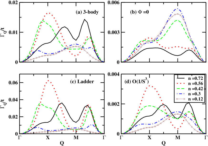
Figure 4: (Color online) Dependence of the spin–wave dephasing rate on the carrier concentration $n$ for $U=0$: comparison between the different approximations of the correlations $J=8t,\gamma=0.2t,\Gamma=U=J_{\rm{AF}}=0$.

To interpret the above results, we turn to the Green’s function equations of motion and note that, for $U$=0, $\Sigma^{U}$=0. After solving Eqs.(20) and (22) for $X$ and $\Phi$ and substituting into Eq.(21) we obtain that

$$\Omega_{\bf\alpha\nu}G_{\alpha\nu}=$$

$$\frac{J}{2N}\frac{\varepsilon_{\bf\nu+Q}-\varepsilon_{\nu}-\omega}{\Delta-i\Gamma+\varepsilon_{\bf\nu+Q}-\varepsilon_{\nu}-\omega}\left(1+\sum_{\beta}G_{\beta\nu}\right)$$

$$-\frac{J}{2N}\sum_{\mu}G_{\alpha\mu}\times$$

$$\frac{\varepsilon_{\bf Q+\mu+\nu-\alpha}-\varepsilon_{\mu}+\varepsilon_{\alpha}-\varepsilon_{\nu}-\omega}{\Delta-i\Gamma+\varepsilon_{\bf Q+\mu+\nu-\alpha}-\varepsilon_{\mu}+\varepsilon_{\alpha}-\varepsilon_{\nu}-\omega},$$ (33)

where

$$\Omega_{\bf\alpha\nu}=\omega+i\gamma-\left(\varepsilon_{\alpha}-\varepsilon_{\nu}\right)$$

$$-\frac{J}{2N}\sum_{\mu}\frac{\varepsilon_{\bf Q+\mu+\nu-\alpha}-\varepsilon_{\mu}+\varepsilon_{\alpha}-\varepsilon_{\nu}-\omega}{\Delta-i\Gamma+\varepsilon_{\bf Q+\mu+\nu-\alpha}-\varepsilon_{\mu}+\varepsilon_{\alpha}-\varepsilon_{\nu}-\omega}.$$ (34)

and $\gamma,\Gamma$ $\rightarrow$0.

Spin–wave dephasing results from the scattering of the magnon of momentum ${\bf Q}$ to momentum ${\bf Q}+{\bf\nu}-{\bf\alpha}$ while an electron is excited from the state ${\bf\nu}$ inside the Fermi sea to the empty state ${\bf\alpha}$. In the limit $\gamma\rightarrow 0$, this magnon–Fermi sea scattering process must satisfy the energy conservation condition $\Omega_{\bf\alpha\nu}=0$, i.e. the initial magnon energy, $\omega=\omega_{{\bf Q}}$, must equal the final state energy that includes the Fermi sea pair energy and the ${\bf Q}+{\bf\nu}-{\bf\alpha}$ magnon energy. The final state magnon energy, given by the last term in Eq.(IV.1), comes from the coupling of $G$ to $\Phi$. For $\Phi$=0, this spin–wave energy is replaced by the local spin excitation energy $Jn/2$. The scattering of small energy Fermi sea pair excitations from right below to right above the Fermi surface dominates the spin–wave lifetime. The density of states and characteristic momenta of such pair excitations depends on the shape of the Fermi surface and therefore on the carrier concentration.

To derive the O($1/S^{3})$ dephasing rate, golosov ; chubukov we neglect all rescattering terms on the rhs of Eq.(IV.1) ($\propto G$). Substituting the expression for $G$ obtained this way into Eq.(28), we obtain the Born approximation self energy

$$\Sigma^{\rm{B}}_{J}=\frac{J^{2}}{4N^{2}}\sum_{\alpha\nu}\left(\frac{\varepsilon_{\bf\nu+Q}-\varepsilon_{\nu}-\omega}{\Delta+\varepsilon_{\bf\nu+Q}-\varepsilon_{\nu}-\omega}\right)^{2}\frac{1}{\Omega_{\alpha\nu}}.$$ (35)

Expanding in terms of 1/S while keeping $\Delta=JS$ fixed and substituting $\omega=\omega^{(1)}_{{\bf Q}}$, where $\omega^{(1)}_{{\bf Q}}$ denotes the $O(1/S)$ spin–wave energy, we obtain the lowest order contribution to the self–energy imaginary part:

$$\rm{Im}\Sigma_{J}^{\rm{B}}(\omega_{{\bf Q}},{\bf Q})\approx\frac{\Delta^{2}}{4N^{2}S^{2}}\sum_{\alpha\nu}\left(\frac{\varepsilon_{\nu}-\varepsilon_{\nu+\bf Q}}{\varepsilon_{\nu}-\varepsilon_{\nu+\bf Q}-\Delta}\right)^{2}{\rm Im}\frac{1}{\Omega_{\alpha\nu}},$$ (36)

where

$$\Omega_{\bf\alpha\nu}=\omega^{(1)}_{{\bf Q}}-\left(\varepsilon_{\alpha}-\varepsilon_{\nu}+\omega^{(1)}_{{\bf Q}-\alpha+\nu}\right)-i\gamma.$$ (37)

The above result corresponds to the Fermi’s golden rule description of the magnon lifetime. Its large difference from our full calculation, demonstrated by Fig.2, is due to the magnon–electron and magnon–hole multiple interactions (vertex corrections), described by the terms proportional to $G$ on the rhs of Eq.(IV.1). The comparison between the different approximations shows that, in the parameter regime of interest in the manganites, the vertex corrections due to three–body correlations renormalize significantly the magnon–carrier scattering.

We finally turn to the dependence of the spin relaxation on the carrier concentration. Fig.4(a) demonstrates a strong $n$–dependence of $\Gamma_{{\bf Q}}$, which correlates with an analogous dependence of $\omega_{{\bf Q}}$ and the spin–wave softening discussed in Ref.[kapet2, ]. As $n$ decreases and the softening (non–Heisenberg behavior) disappears, the spin–wave lifetime increases while its momentum dependence changes. For intermediate $n$, $\Gamma_{{\bf Q}}$ displays two sharp peaks and a dip as function of momentum. For small $n$, the overall $\Gamma_{{\bf Q}}$ decreases and the positions of its maxima and minima change.

To see this concentration dependence in more detail, we note that, for $n=0.72$, the spin–wave damping is maximized for ${\bf Q}\sim(\pi,\pi/2)$, between $X$ and $M$, and ${\bf Q}\simeq(\pi,\pi/2)$, between $M$ and $\Gamma$, while it is minimized close to the $M$ point. As $n$ decreases to intermediate values, the first of the above maxima approaches the $X$–point while the second maximum shifts closer to ${\bf Q}=(\pi,\pi/2)$. For smaller $n$, the dip close to the $M$ point turns into a maximum. As a result of this $n$–dependence, $\Gamma_{{\bf Q}}/\omega_{{\bf Q}}$ becomes quite large in the direction $\Gamma\to X$ for intermediate $n$, which implies that these spin–wave quasi–particles interact strongly with the Fermi sea. For small $n$, $\Gamma_{{\bf Q}}/\omega_{{\bf Q}}$ decreases again. The changes in the momentum dependence with $n$ are related to the changes in the shape and position of the Fermi surface, which is located close to the Brillouin zone boundary for the higher $n$ but moves towards the center of the Brillouin zone as $n$ decreases. As a result, the phase space available for magnon–carrier scattering changes drastically with $n$.

Fig.4 also compares the concentration dependence of $\Gamma_{{\bf Q}}$ predicted by the different approximations of the spin–charge interactions. By comparing the full three–body calculation with the O($1/S^{3}$) Fermi’s golden rule result, it is clear that the spin–wave damping is grossly underestimated by the perturbative 1/S expansion for all concentrations. Figs.4(b), obtained by setting $\Phi$=0, fails completely to capture the correct concentration dependence (compare Figs.4(a) and 4(b)). It also predicts very small dephasing rates for all $n$. The above approximation neglects the interactions between Fermi sea pair and carrier spin–flip excitations. We therefore conclude that such carrier–carrier interactions strongly affect the magnetization relaxation. Finally, the comparison of Figs.4(a) and (c) shows that the two–body ladder approximation grossly overestimates the spin–wave damping for intermediate or high $n$, while the discrepancies from the full three–body calculation decrease for small $n$. We conclude based on Fig.4 that the collective spin relaxation predicted by the minimal double–exchange model can be controlled by tuning the carrier concentration $n$, by doping or with external probes. Such tuning is heavily influenced by the correlations, which must be treated accurately in order to capture even the correct order of magnitude and momentum dependence of the spin dephasing rate for all concentrations.

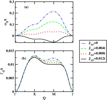
Figure 5: (Color online) Role of the super–exchange interaction $J_{\rm{AF}}$. (a) Spin–wave dispersion and (b) Spin–wave damping rate. $J=2t,U=10t,n=0.6,\Gamma=0.5t,\gamma=0.2t$

IV.2 The role of the Coulomb Repulsion

In this section we study how the on–site Coulomb repulsion, $U$, and direct superexchange interaction, $J_{AF}$, affect the spin–wave energies and lifetimes. Fig.5 compares the results obtained for different values of $J_{\rm{AF}}/t$ within the range $0\leq J_{AF}\leq 0.012t$ relevant to the manganites.dagotto $J_{\rm{AF}}$ leads to an overall softening of the spin–wave energies. These eventually turn negative, implying instability of the fully polarized ferromagnetic phase. However, $J_{AF}$ preserves the nearest neighbor Heisenberg model momentum dependence, unlike for the softening observed in the experiment.ye Also, it does not affect the spin damping in a significant way. We take $J_{\rm{AF}}=0$ from now on.

As demonstrated by Fig.6, the effects of the on–site Coulomb (Hubbard) repulsion $U$ are more significant. Fig.6(a) shows the dependence of the spin–wave dispersion on $U$. With increasing $U$, the spin–wave softening and deviations from the Heisenberg model dispersion diminish as the ferromagnetic phase becomes more stable. As discussed in Ref.[kapet2, ], our calculated dispersion can be fitted to the Heisenberg model dispersion with first– and fourth–nearest–neighbor interactions, similar to the experiment. ye Fig.6(b) demonstrates qualitative changes in the overall momentum dependence of the spin–wave damping as compared to the minimal double exchange model. In particular, if the carrier spin is conserved ($\Gamma$=0), $\Gamma_{{\bf Q}}$ is maximum at the $M$ point, while the damping at the $X$ point is smaller. In contrast, for $U=0$ and intermediate concentrations, the dephasing rate displays a dip at the $M$ point and is maximum close to the $X$ point (see e.g. Fig.3). The double–peak momentum dependence of $\Gamma_{{\bf Q}}$ for $U$=0 can be recovered for large $U$ only by introducing a sufficiently large itinerant spin damping rate $\Gamma$ (see Fig.6(c)). The experiment of Ref.[ye, ] observed an increase in the spin–wave damping along $\Gamma\to M$ that exceeds the corresponding increase along $\Gamma\to X$, similar to our results for finite $U$ and $\Gamma$=0 (Fig.6(b)). Our calculations show that such behavior of the spin damping can be attributed to the Coulomb repulsion $U$ in the intrinsic system ($\Gamma,\gamma\rightarrow$0) described by the Hamiltonian $H$.

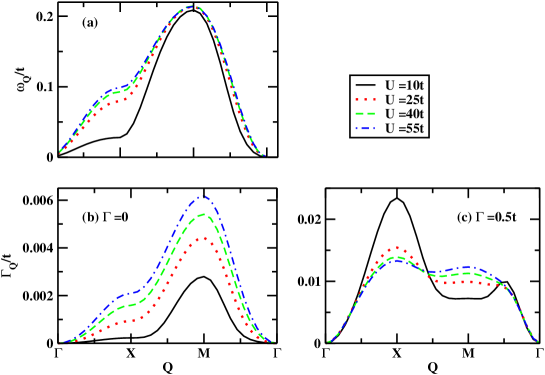
Figure 6: (Color online) Effects of the on–site Coulomb repulsion $U$. (a) Spin–wave dispersion, (b) Spin–wave damping rate for $\Gamma=0$, and (c) (b) Spin–wave damping rate for $\Gamma$=0.5$t$. $n=0.6,J=2t,\gamma=0.2t,J_{\rm{AF}}=0$.

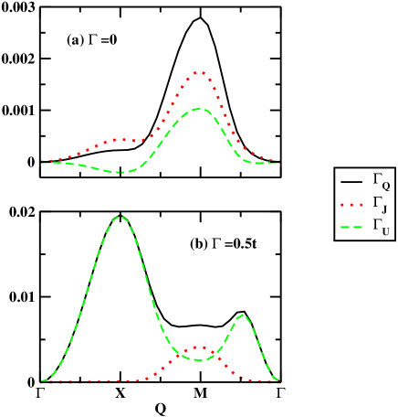
Figure 7: (Color online) Contributions $\Gamma_{{\bf Q}}^{J}$ and $\Gamma_{{\bf Q}}^{U}$ to the inelastic spin–wave dephasing rate $\Gamma_{{\bf Q}}$. (a) $\Gamma=0$, (b) $\Gamma$=0.5t. $n$=0.6, $J$=2$t$, $U$=10$t$, $\gamma$=0.2$t$, $J_{AF}=0$.

Fig.6 also demonstrates a qualitative difference in the dependence of $\Gamma_{{\bf Q}}$ on $U$ between the cases of small and large itinerant spin damping. For $\Gamma$=0, the spin–wave dephasing rate increases with $U$ (Fig.6(b)), while for $\Gamma$=0.5$t$ it decreases with $U$ close to the $X$–point (Fig.6(c)). This result indicates that the magnetization relaxation may depend on the interplay between Coulomb repulsion and the dephasing of the itinerant spin via the coupling to an external bath.

To interpret the above behaviors, we plot in Fig.7 the two contributions to $\Gamma_{{\bf Q}}$ obtained from the self energies Eqs.(28) and (29) for zero and finite $\Gamma$. $\Gamma^{J}$ is determined by $G$, while $\Gamma^{U}$ is determined by $\Phi$. For $\Gamma$=0, Fig.7(a) shows that $\Gamma^{J}$ and $\Gamma^{U}$ are comparable in magnitude, since in this case they both arise from $\rm{Im}$G. On the other hand, as $\Gamma$ increases, the relative magnitude of $\Gamma^{J}$ and $\Gamma^{U}$ changes and the latter dominates (see Fig.7(b)). This enhancement of $\Gamma^{U}$ arises from the additional contribution to $\rm{Im}\Phi$, Eq.(22), obtained by adding the relaxation rate $\Gamma$ to Eq.(22). Even though $\Gamma^{J}$ continues to have the same momentum dependence as for $\Gamma$=0, $\Gamma^{U}$ does not (compare Figs.7(a) and 7(b)).

Fig.8 shows the dependence of the two contributions to the inelastic dephasing rate on the Coulomb repulsion for large $U$ and different $\Gamma$. $\Gamma^{J}$ increases and then saturates with increasing $U$. For $\Gamma$=0 (intrinsic system), $\Gamma^{U}$ increases with $U$ and eventually exceeds $\Gamma^{J}$. Unlike for $\Gamma^{J}$, the dependence of $\Gamma^{U}$ on the momentum and on $U$ is qualitatively different for large and small $\Gamma$. For example, $\Gamma^{U}$ decreases with $U$ at the $X$–point for large $\Gamma$ but increases for $\Gamma$=0. The above behavior of $\Gamma^{U}$ dominates the total dephasing rate for large $\Gamma$.

Fig.9(a) shows the transition in the momentum dependence of $\Gamma_{{\bf Q}}$ as $U$ increases for $\Gamma$=0. This transition occurs around $U\sim$6$t$, where the double peak momentum dependence for $U$=0, with a dip at the $M$–point, changes into a peak at the $M$–point. As can be seen in Fig.9(b), the above transition arises from the changes in the behavior of $\Gamma^{J}$, determined by the Green’s function $G$ (Eq.(21)), that are introduced by the Coulomb repulsion. Fig.9(c), on the other hand, shows that the overall momentum dependence of $\Gamma^{U}$ remains approximately the same for all $U$.

Finally, we turn to the possibility of controlling the magnetization relaxation by tuning the carrier concentration $n$ and study how the Hubbard repulsion $U$ changes the picture as compared to the prediction of Fig.4. Fig.10 shows the dependence of the dispersion and spin damping rate on $n$ within a wide range of concentrations, $n=0.7-0.1$. As can be seen in Fig.10(a), the pronounced softening along the $\Gamma$–$X$ direction disappears rapidly with decreasing $n$ (or increasing hole doping $x$=1-$n$). For small values of $n$, the overall energies decrease and the overall shape of the dispersion changes.

The above $n$–dependence of the spin–wave dispersion correlates with corresponding changes in the dephasing rate. Fig.10(b), obtained for $\Gamma$=0, shows that the Coulomb repulsion $U$ changes drastically the dependence of $\Gamma_{{\bf Q}}$ on $n$ as compared to the predictions of the minimal double exchange model, Fig.4(a). In this case, the spin dephasing rate increases as $n$ decreases to intermediate values, in a way correlated with the disappearance of the spin–wave softening and non–Heisenberg behavior. For small $n$, where the softening has disappeared and the overall energies start to decrease, the spin damping rate also decreases. Furthermore, unlike for $U$=0 or for large $\Gamma$, $\Gamma_{{\bf Q}}$ displays a strong maximum at point $M$ for all concentrations and is always weaker along the $\Gamma$–$X$ direction. As can be seen by comparing Figs.10(a) and (b), a sufficiently short itinerant spin lifetime (large $\Gamma$) changes drastically the momentum dependence of $\Gamma_{{\bf Q}}$ and its dependence on $n$.

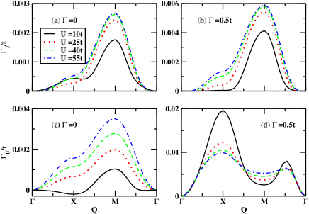
Figure 8: (Color online) Dependence of $\Gamma_{{\bf Q}}^{J}$ and $\Gamma_{{\bf Q}}^{U}$ on Coulomb repulsion for large $U$. $n$=0.6, $J$=2$t$, $\gamma$=0.2$t$, $J_{AF}=0$.

We conclude based on Fig.10 that the magnitude and momentum dependence of $\Gamma_{{\bf Q}}$, as well as the spin–wave softening, can be controlled by tuning the carrier concentration $n$, via hole doping or by external means such as photoexcitation. bigot-05 ; kampen ; kimel-anis ; tolk ; lupke ; kimel-rev ; wang-rev ; shah ; chovan It is clear that the on–site Coulomb (Hubbard) repulsion plays a dominant role, by inducing new correlations and dynamics absent in the simple double–exchange model. Such correlations change drastically the momentum dependence and magnitude of $\Gamma_{{\bf Q}}$ with varying $n$ and must be treated in a consistent way in order to arrive at trustworthy conclusions and comparisons to experiment. Our results suggest that, as a first step, a systematic experimental study of the magnetization dynamics as function of doping $x$ and a comparison to the theory is necessary in order to decide which many–body mechanisms dominate the collective magnetization dynamics and relaxation and learn how to control this dynamics for potential magnetic device and spintronics applications.

V Conclusions

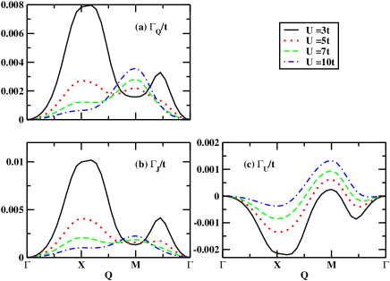
Figure 9: (Color online) Dependence of (a) $\Gamma_{{\bf Q}}$, (b) $\Gamma_{{\bf Q}}^{J}$, (c) $\Gamma_{{\bf Q}}^{U}$ on the Coulomb repulsion for small $U$. $n$=0.6, $J$=4$t$, $\gamma$=0.2$t$, $J_{AF}=\Gamma=0$.

In this paper we presented a general method for describing the spin–wave dynamics and relaxation in itinerant ferromagnets. This method is based on a correlation expansion of the Green’s function equations of motion that systematically treats all correlations between any given number of elementary excitations. Using this method, we derived a closed system of equations that treat the magnetic exchange and Coulomb interactions non–perturbatively and solved it to obtain the Green’s function that determines the transverse spin susceptibility. Our results for the spin–wave dispersion reproduce previous variational kapet1 ; kapet2 and exact diagonalization exact ; igar results (in the limit $\Gamma$,$\gamma$ $\rightarrow$0) and therefore allow us to draw definite conclusions regarding the magnitude of the spin–wave softening. Using the properties of the fully polarized Hartree–Fock ground state with maximum spin, we showed that our method gives the exact spin Green’s function within a subspace of states that include up to one Fermi sea pair excitation. Our factorization scheme of the higher Green’s functions also applies to other ground states. Our results recover the 1/S expansion results as special case. We showed that, in the parameter regime of interest in the manganites, the latter approximation overestimates the spin–wave softening, while at the same time it grossly underestimates the spin–wave damping rate. Furthermore, by comparing with the ladder approximation treatment of the vertex corrections to the magnon–carrier scattering, which treats the multiple magnon–electron scatterings while neglecting the interactions with a Fermi sea hole, we showed that three–body correlations between the magnon and an electron–hole Fermi sea pair excitation have an important effect on the spin relaxation.

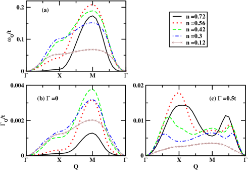
Figure 10: (Color online) Dependence of spin–wave dispersion and dephasing rate on the carrier concentration $n$ for $U$=10$t$. (a) dispersion, (b) dephasing rate for $\Gamma$=0, (c) dephasing rate for $\Gamma$=0.5$t$. $J=2t,J_{\rm{AF}}=0,\gamma=0.2t$.

Using the above many–body theory, we calculated the inelastic spin–wave dephasing rate non–perturbatively in the interactions and 1/S (i.e. beyond the standard Fermi’s Golden Rule). We showed that correlations between a carrier spin–flip excitation and a Fermi sea pair induced by the Coulomb repulsion $U$ play a very important role in the parameter regime relevant to the manganites. We also showed that both the magnitude and momentum dependence of the spin–wave dephasing rate depend sensitively on the itinerant carrier concentration. This result implies the possibility of controlling the magnetization relaxation in itinerant ferromagnets by tuning the carrier concentration, either via doping or by external means (e.g. photoexcitation or by using electric fields and currents or gates). We also argued that the interplay between on–site Coulomb (Hubbard) interaction and a finite itinerant carrier spin lifetime, due to the coupling of the different spin states induced by spin–orbit or other interactions not included in our Hamiltonian, can affect our results in the realistic system. The momentum dependence of the spin–wave dephasing rate observed in recent experiments ye is consistent with the results of our calculation only for sufficiently large $U$ and $\Gamma\rightarrow$0. In all other cases, we obtain a distinctly different double peak momentum dependence. Although the bandstructure of the relevant materials must be included in order to arrive at quantitative comparisons with the experiment, our calculation already demonstrates the crucial role of correlations. The agreement of the main trends in spin–wave softening and damping rate changes as function of $n$ between our theory and the experiment suggests that the simple one–band model already contains the main inelastic scattering processes and correlations. Our results suggest that ultrafast magneto–optical pump–probe spectroscopy experiments, which directly probe the changes in spin relaxation and dynamics induced by photoexcited carriers,chovan may provide new insight into the physics of the manganites and other itinerant ferromagnetic systems.

This work was supported by the EU STREP program HYSWITCH.

References

- (1) E. L. Nagaev, Phys. Rep. 346, 387 (2001).
- (2) See e.g. Colossal Magnetoresistance Oxides, ed. Y. Tokura (Gordon Breach, Singapore, 2000) and references therein.
- (3) See e.g. Y. Tokura, Physics Today 50, July 2003.
- (4) T. Jungwirth, J. Sinova, J. Masek, J. Kucera, amd A. H. MacDonald, Rev. Mod. Phys. 78, 809 (2006).
- (5) S. A. Wolf, D. D. Awschalom, R. A. Buhrman, J. M. Daugherton, S. von Molnar, M. L. Roukes, A. Y. Chtchelkanova, and D. M. Treger, Science 294, 1488 (2001).
- (6) Y. Tserkovnyak, A. Brataas, G. Bauer, and B. I. Halperin, Rev. Mod. Phys. 77, 1375 (2005).
- (7) B. Heinrich, D. Fraitova, and V. Kambersky, Phys. Status Solidi 23, 501 (1967).
- (8) A. H. Mitchell, Phys. Rev. 105, 1439 (1957).
- (9) J. Sinova, T. Jungwirth, X. Liu, Y. Sasaki, J.K. Furdyna, W.A. Atkinson, and A.H. MacDonald, Phys. Rev. B 69, 085209 (2004).
- (10) Y. Tserkovnyak, G. A. Fiete, and B. I. Halperin, Appl. Phys. Lett. 84, 5234 (2004).
- (11) N. Furukawa, J. Phys. Soc. Jpn. 65, 1174 (1996).
- (12) X. Wang, Phys. Rev. B 57, 7427 (1998).
- (13) E. L. Nagaev, Phys. Rev. B 58, 827 (1998)
- (14) D. I. Golosov, Phys. Rev. Lett. 84, 3974 (2000); Phys. Rev. B 71, 014428 (2005).
- (15) S.–J. Sun, W.–C. Lu, and H. Chou, Physica B 324, 286 (2002).
- (16) M. Marder, N. Papanicolaou, and G. C. Psaltakis, Phys. Rev. B 41, 6920 (1990); L. R. Mead and N. Papanicolaou, Phys. Rev. B 28, 1633 (1983).
- (17) J.Chovan, E.G. Kavousanaki, and I. E. Perakis, Phys. Rev. Lett. 96, 057402 (2006); J.Chovan and I. E. Perakis, Phys. Rev. B 77, 085321 (2008); J.Chovan, E.G. Kavousanaki, and I. E. Perakis, Phys. Stat. Sol. C 3, 2410 (2006).
- (18) V. Yu. Irkhin and M. I. Katsnelson, Eur. Phys. J. B 19, 401 (2001) and references therein.
- (19) N. Shannon and A. V. Chubukov, Phys. Rev. B 65, 104418 (2002); J. Phys. Cond. Matt. 14, L235 (2002).
- (20) M. Vomir, L. H. F. Andrade, L. Guidoni, E. Beaurepaire, and J.-Y. Bigot, Phys. Rev. Lett. 94, 237601 (2005).
- (21) M. van Kampen, C. Jozsa, J. T. Kohlhepp, P. LeClair, L. Lagae, W. J. M. de Jonge, and B. Koopmans, Phys. Rev. Lett. 88, 227201 (2002).
- (22) A. V. Kimel, A. Kirilyuk, A. Tsvetkov, R. V. Pisarev, and Th. Rasing, Nature 429, 850 (2004).
- (23) J. Qi, Y. Xu, N. H. Tolk, X. Liu, J. K. Furdyna, and I. E. Perakis, Appl. Phys. Lett. 91, 112506 (2007).
- (24) D. Talbayev, H. Zhao, G. Lüpke, A. Venimadhav, and Qi Li, Phys. Rev. B 73, 014417 (2006).
- (25) A. V. Kimel, A. Kirilyuk, F. Hansteen, R. V. Pisarev, and Th. Rasing, J. Phys. Condens. Matter 19, 043201 (2007).
- (26) J. Wang, C. Sun, Y. Hashimoto, J. Kono, G. A. Khodaparast, L. Cywinski, L. J. Sham, G. D. Sanders, C. Stanton, and H. Munekata, J. Phys. Cond. Matt. 18, R501 (2006).
- (27) T. V. Shahbazyan, I. E. Perakis, and M. E. Raikh, Phys. Rev. Lett. 84, 5896 (2000).
- (28) C. S. Zener, Phys. Rev. 82, 403 (1951); P. W. Anderson and H. Hasegawa, Phys. Rev. 100, 675 (1955); P. G. de Gennes, Phys. Rev. 100, 564 (1955); K. Kubo and N. Ohata, J. Phys. Soc. Jpn. 33, 21 (1972).
- (29) E. Dagotto, T. Hotta, and A. Moreo, Phys. Rep. 344, 1 (2001).
- (30) M. D. Kapetanakis, and I. E. Perakis, Phys. Rev. B, 75, 140401(R) (2007).
- (31) T. G. Perring, G. Aeppli, S. M. Hayden, S. A. Carter, J. P. Remeika, and S.-W. Cheong, Phys. Rev. Lett. 77, 711 (1996).
- (32) H. Y. Hwang, P. Dai, S.-W. Cheong, G. Aeppli, D. A. Tennant, and H. A. Mook, Phys. Rev. Lett. 80, 1316 (1998).
- (33) P. Dai, H. Y. Hwang, J. Zhang, J. A. Fernandez-Baca, S.-W. Cheong, C. Kloc, Y. Tomioka, and Y. Tokura, Phys. Rev. B 61, 9553 (2000).
- (34) L. Vasiliu-Doloc, J. W. Lynn, A. H. Moudden, A. M. de Leon-Guevara, and A. Revcolevschi, Phys. Rev. B 58, 14913 (1998).
- (35) T. Chatterji, L. P. Regnault, and W. Schmidt, Phys. Rev. B 66, 214408 (2002).
- (36) Y. Endoh, H. Hiraka, Y. Tomioka, Y. Tokura, N. Nagaosa, and T. Fujiwara, Phys. Rev. Lett. 94, 017206 (2005).
- (37) T. Chatterji, L. P. Regnault, P. Thalmeier, R. Suryanarayanan, G. Dhalenne, and A. Revcolevschi, Phys. Rev. B 60, R6965 (1999).
- (38) N. Shannon, T. Chatterji, F. Ouchni, and P. Thalmeier, Eur. Phys. J. B 27, 287 (2002).
- (39) F. Ye, P. Dai, J. A. Fernandez–Baca, H. Sha, J. W. Lynn, H. Kawano–Furukawa, Y. Tomioka, Y. Tokura, and J. Zhang, Phys. Rev. Lett. 96, 047204 (2006); F. Ye, P. Dai, J. A. Fernandez–Baca, D. T. Adroja, T. G. Perring, Y. Tomioka, and Y. Tokura, Phys. Rev. B. 75, 144408 (2007).
- (40) G. Khaliullin and R. Kilian, Phys. Rev. B 61, 3494 (2000).
- (41) M. D. Kapetanakis, A. Manousaki, and I. E. Perakis, Phys. Rev. B, 73, 174424, (2006).
- (42) D. M. Edwards, Adv. Phys. 51, 1259 (2002).
- (43) Y. Motome and N. Furukawa, Phys. Rev. B 71, 014446 (2005).
- (44) I. V. Solovyev and K. Terakura, Phys. Rev. Lett. 82, 2959 (1999).
- (45) T. A. Kaplan, S. D. Mahanti, and Y.–S. Su,. Phys. Rev. Lett. 86, 3634 (2001).
- (46) J. Zang. H. Röder, A. R. Bishop, and S. A. Trugman, J. Phys. Cond. Matt. 9, L157 (1997); T. A. Kaplan and S. D. Mahanti, J. Phys. Cond. Mat. 9, L291 (1997).
- (47) J. Igarashi, J. Phys. Soc. Jpn 52, 2827 (1983); J. Igarashi, J. Phys. Soc. Jpn 54, 260 (1985); J. Igarashi, M. Takahashi, and T. Nagao, J. Phys. Soc. Jpn 68, 3682 (1999).
- (48) A. E. Ruckenstein and S. Schmitt–Rink, Int. J. Mod. Phys. B 3, 1809 (1989).
- (49) I. E. Perakis and E. G. Kavousanaki, Chem Phys. 318, 118 (2005); A. T. Karathanos, I. E. Perakis, N. A. Fromer, and D. S. Chemla, Phys. Rev. B 67, 035316 (2003); K. M. Dani, E. G. Kavousanaki, J. Tignon, D. S. Chemla, and I. E. Perakis, Solid State Commun. 140, 72 (2006).
- (50) J. Fricke, Annals Phys. 252, 479 (1996); J. Fricke, V. Meden, C. Wohler, and K. Schönhammer, Annals Phys. 253, 177 (1997); V. Meden, C. Wohler, J. Fricke, and K. Schönhammer, Phys. Rev. B 52, 5624 (1995).
- (51) M. D. Kapetanakis and I. E. Perakis, Phys. Rev. Lett. 101, 097201 (2008).
- (52) J. F. Mueller, A. E. Ruckenstein, and S. Schmitt–Rink, Phys. Rev. B 45, 8902 (1992); A. E. Ruckenstein and S. Schmitt–Rink, ibid. 35, 7551 (1987).
- (53) I. E. Perakis and Y.–C. Chang, Phys. Rev. B 47, 6573 (1993); ibid 44, 5877 (1991).
- (54) T. V. Shahbazyan, N. Primozich, I. E. Perakis, and D. S. Chemla, Phys. Rev. Lett. 84, 2006 (2000); N. Primozich, T. V. Shahbazyan, I. E. Perakis, and D. S. Chemla, Phys. Rev. B 61, 2041 (2000).
- (55) S. V. Tyablikov, Methods in the quantum theory of magnetism, (Plenum press, New York, 1967)
- (56) W. von der Linden and D. M. Edwards, J. Phys. : Condens. Matter 3, 4917 (1991).