Distance, Growth Factor, and Dark Energy Constraints from Photometric Baryon Acoustic Oscillation and Weak Lensing Measurements
Abstract
Baryon acoustic oscillations (BAOs) and weak lensing (WL) are complementary probes of cosmology. We explore the distance and growth factor measurements from photometric BAO and WL techniques and investigate the roles of the distance and growth factor in constraining dark energy. We find for WL that the growth factor has a great impact on dark energy constraints but is much less powerful than the distance. Dark energy constraints from WL are concentrated in considerably fewer distance eigenmodes than those from BAO, with the largest contributions from modes that are sensitive to the absolute distance. Both techniques have some well determined distance eigenmodes that are not very sensitive to the dark energy equation of state parameters and , suggesting that they can accommodate additional parameters for dark energy and for the control of systematic uncertainties. A joint analysis of BAO and WL is far more powerful than either technique alone, and the resulting constraints on the distance and growth factor will be useful for distinguishing dark energy and modified gravity models. The Large Synoptic Survey Telescope (LSST) will yield both WL and angular BAO over a sample of several billion galaxies. Joint LSST BAO and WL can yield level precision on ten comoving distances evenly spaced in between redshift and with cosmic microwave background priors from Planck. In addition, since the angular diameter distance, which directly affects the observables, is linked to the comoving distance solely by the curvature radius in the Friedmann-Robertson-Walker metric solution, LSST can achieve a pure metric constraint of 0.017 on the mean curvature parameter of the universe simultaneously with the constraints on the comoving distances.
Subject headings:
cosmological parameters — distance scale — gravitational lensing — large-scale structure of universe1. Introduction
The luminosity distance–redshift relation measured from type Ia supernovae (SNe) has provided a vital piece of evidence for an accelerated cosmic expansion in a Friedman-Robertson-Walker universe (Riess et al. 1998; Perlmutter et al. 1999). Such an acceleration suggests that either the universe is dominated by a smooth dark energy component or we need an alternative framework of gravity to account for the SN data (e.g., Dvali et al. 2000; Deffayet 2001). Although different answers have vastly different theoretical implications, they can only be distinguished indirectly, for example, through measurements of the cosmic distance scale as a function of redshift and the amplitude of the density fluctuations as a function of redshift, i.e., the growth factor–redshift relation. One may further derive a phenomenological dark energy equation of state (EOS) as a function of redshift, , from the distances and growth factors and contrast it with predictions from theory.
Besides SNe, baryon acoustic oscillations (BAOs) in the galaxy power spectrum (Eisenstein, Hu, & Tegmark 1998; Cooray et al. 2001; Blake & Glazebrook 2003; Hu & Haiman 2003; Linder 2003) and weak lensing (WL, Hu & Tegmark 1999; Mellier 1999; Bartelmann & Schneider 2001; Huterer 2002; Refregier 2003; Song & Knox 2004) can also measure the distance (Seo & Eisenstein 2003; Song 2005; Knox, Song, & Tyson 2006a; Zhan & Knox 2006a). The sound horizon at the last scattering surface determines the BAO scale (Peebles & Yu 1970; Bond & Efstathiou 1984; Holtzman 1989), which is fixed in comoving space, so that it can be used as a standard ruler to measure the comoving angular diameter distance and, with spectroscopy, Hubble parameter . With precise calibration of the sound horizon from cosmic microwave background (CMB) observations, the BAO technique is able to measure the absolute distance, whereas the SN technique measures the relative distance because of the degeneracy between the SN intrinsic luminosity and the Hubble constant . The WL technique does not depend on power spectrum features; its ability to measure distance originates from its geometric lensing kernel and the sensitivity of the shear power spectrum amplitude to the absolute distance (e.g., Zhan & Knox 2006b, hereafter ZK06b).
The WL shear signal is a direct indicator of the gravitational potential of all matter, luminous or not, so the WL technique has the advantage of being able to measure the growth factor of the large-scale structure directly. For the BAO technique111Although the BAO features are not related to the growth factor, the BAO technique, being a power spectrum or correlation function analysis, can potentially measure the growth factor., the growth factor is largely degenerate with the galaxy clustering bias, though it could be determined from the shape of the galaxy power spectrum if one knew precisely how the amplitude of the linear matter power spectrum affects the slope of the nonlinear matter power spectrum and how the galaxy bias behaves in the mildly nonlinear regime (see Section 3.2).
The relative importance of the distance and growth factor in constraining the dark energy EOS with WL has been discussed by Abazajian & Dodelson (2003), Simpson & Bridle (2005, hereafter SB05), Zhang, Hui, & Stebbins (2005, hereafter ZHS05), and Knox et al. (2006a), but their results are apparently inconsistent: SB05 and ZHS05 argue that the distance and growth factor are equally powerful whereas Abazajian & Dodelson (2003) and Knox et al. (2006a) show that the growth factor is much less powerful than the distance. This inconsistency is found to be caused by the parameter space of each analysis: with no other parameters, the distance and growth factor place comparable constraints on the dark energy EOS parameters, but the growth factor becomes less powerful when more parameters are allowed to float (ZK06b). Because the WL measurements of the distance and growth factor are entangled, ambiguity arises on the exact meaning of “using only the distance (or growth) information” without a reconstruction of distances and growth factors (actually, their errors). In this paper, we give a detailed account of estimating the distance and growth errors and their roles in constraining dark energy.
Throughout this paper, we assume a low-density cold dark matter (CDM) universe with the following parameters: the dark energy equation-of-state parameters and as defined by (Chevallier & Polarski 2001), the matter density , the baryon density , the angular size of the sound horizon at the last scattering surface , the equivalent matter fraction of curvature , the optical depth to scattering by electrons in the reionized inter-galactic medium, , the primordial helium mass fraction , the spectral index and running of the primordial scalar perturbation power spectrum, and the normalization of the primordial curvature power spectrum at . For reasons stated in Section 3.1, only a subset of these parameters are retained when distance and growth parameters are present. The fiducial model is taken from the 3-year WMAP data (Spergel et al. 2007): (, , , , , , , , , , ) = (-1, 0, 0.127, 0.0223, 0.596∘, 0, 0.09, 0.24, 0.951, 0, ). The reduced Hubble constant and the present equivalent matter fraction of dark energy are implicit in this parametrization, meaning that either one of them can replace or any parameter that affects .
The rest of the paper is organized as follows. Section 2 provides a brief introduction to the power spectrum analysis and error forecast with BAO and WL. For the investigation that follows, we assume a photometric redshift (photo-z) survey based on the Large Synoptic Survey Telescope222See http://www.lsst.org. (LSST, Ivezic et al. 2008) and consider only photo-z BAO and WL tomography. We compare BAO and WL constraints on the distance and growth factor in Section 3 and examine the roles of distance and growth for studying dark energy in Section 4. The conclusions are drawn in Section 5. Since our main goal is to understand the intrinsic properties of the distance and growth factor measured from the two techniques and their applications in dark energy studies, we neglect systematics in Sections 3 and 4. To be more realistic, we include in Section 5 a brief discussion of the constraints on the distance and growth factor from a joint analysis of LSST BAO and WL with conservative estimates of systematic uncertainties in photo-zs and power spectra. For more detailed accounts of various systematics, see Huterer & Takada (2005); White (2005); Ma, Hu, & Huterer (2006); Huterer et al. (2006); Jain, Jarvis, & Bernstein (2006); Zhan (2006); Eisenstein, Seo, & White (2007); Guzik, Bernstein, & Smith (2007); Zentner, Rudd, & Hu (2008).
2. Weak Lensing and Baryon Acoustic Oscillations
The projected lensing potential transforms a small displacement in the source plane into a small displacement in the image plane via (Kaiser 1992; Bartelmann & Schneider 2001)
where the convergence , the shear components and . The shear represents the distortion of an image without magnification, so that it can be inferred from the average ellipticity of galaxies within an appropriate window under the assumption that galaxies are randomly oriented in the absence of lensing. One may decompose a shear map into E-modes and B-modes, but, to first order, gravitational lensing from density fluctuations does not induce B-modes. Therefore, we only consider the E-mode shear statistics here.
The angular power spectra of the shear and galaxy number density can be written as (Hu & Jain 2004; Zhan 2006)
| (1) |
where lower case subscripts correspond to the tomographic bins, upper case superscript labels the observables, e.g., for galaxies or for shear, is the dimensionless power spectrum of the density field, is the comoving angular diameter distance of redshift as viewed from redshift 0 [the same as the comoving distance, , between redshift 0 and in a flat universe], and . In the linear regime, the power spectrum is scaled by the growth factor
The window functions are
where is the linear galaxy clustering bias, , and is the comoving angular diameter distance of redshift as viewed from [the same as the comoving distance, , between redshift and in a flat universe]. The galaxy redshift distribution in the th tomographic bin is an average of the underlying three-dimensional galaxy distribution over angles, and the mean surface density is the total number of galaxies per steradian in bin . The binning for WL need not be the same as that for BAO. The irreducible occurrence of the Hubble parameter in equation (1) for BAO is due to the fact that the galaxy number density is measured in redshift not in distance.
Equation (1) is applicable to the shear power spectrum for WL (), galaxy power spectrum for BAO (), and galaxy-shear power spectrum ( and ). Although we focus on gaining a better understanding of the BAO and WL techniques by exploring their differences, we must emphasize that a joint analysis of BAO and WL with all the three types of power spectra (Hu & Jain 2004; Zhan 2006) is far more powerful than either technique alone.
We parametrize the underlying galaxy redshift distribution as (Wittman et al. 2000)
and adopt the values , , and with a projected galaxy number density of per square arcminute for LSST. The galaxy distribution in the th bin is sampled from by (Ma et al. 2006; Zhan 2006)
where the subscript p denotes photo-z space, and define the extent of bin , and is the probability of assigning a galaxy that is at true redshift to the photo-z bin between and . We approximate the photo-z error to be Gaussian with bias and rms , and the probability becomes
The normalization implies that galaxies with a negative photo-z have been excluded from . Although uncertainties in the photo-z parameters and have a large impact on the dark energy constraints from WL (Huterer et al. 2006; Ma et al. 2006; Zhan 2006), such systematic effects are not relevant to how WL probes dark energy. Hence, we fix and per galaxy. In Section 5 we show results with photo-z and power spectrum systematics.
Assuming that the observables, e.g., the shear map in multipole space, and the likelihood of the parameters of interest, q, near the fiducial model are both Gaussian, one can use the Fisher information matrix to estimate the errors of the parameters from the covariance, C, of the observables. In summary, the Fisher matrix is given by (Tegmark 1997)
| (2) |
For BAO and WL tomography, we have
where is the Kronecker delta function, is the rms shear per galaxy for WL, and for BAO. The Gaussian likelihood of the parameters is
where corresponds to the fiducial model and is the covariance of the parameters. The minimum marginalized error of is . Independent Fisher matrices are additive; a prior on , , can be introduced via . A Fisher matrix of the parameters q can be projected onto a new set of parameters p via
| (3) |
3. Distance and Growth Factor Constraints
The distance–redshift and growth factor–redshift relations are the two most important diagnostics of the driving mechanism of the accelerated cosmic expansion, be it dark energy or modified gravity. Various dark energy probes are essentially probes of these relations (and hence they are modified gravity probes as well). Most models of dark energy and modified gravity do not modify the form of equation (1). As such, reconstructing the distance and growth factor from the shear and galaxy power spectra is fairly model-independent, which is useful for distinguishing those models (Lue, Scoccimarro, & Starkman 2004; Song 2005; Ishak, Upadhye, & Spergel 2006; Knox et al. 2006a; Jain & Zhang 2007; but cf. Linder 2004; Bertschinger & Zukin 2008).
To reconstruct the distance and growth factor, one would set a series of distance and growth parameters covering a range of redshifts, interpolate the continuous distance and growth functions from a realization of these parameters, assign a probability of the observed data given the particular set of distance, growth, and other parameters, and repeat the process for enough realizations to map the posterior distribution of all the parameters. This is rather involved. However, if the purpose is to roughly estimate the errors without the actual observational data, one often approximates the posterior distribution of the parameters as a multivariate Gaussian around its peak and applies the Fisher matrix analysis to infer the errors. We show here an example of estimating the errors of reconstructed distances and growth factors from BAO and WL, both separately and in combination.
3.1. Parameters
There is a minor ambiguity in the growth factor of the large-scale structure, and we choose the convention that in an Einstein-de Sitter universe but in general. For distance parameters, it is convenient to use the comoving distance instead of the comoving angular diameter distance . The reason is that while holds all the time, in the presence of curvature:
| (4) |
where . Separately, the freedom of the Hubble parameter, , in the galaxy power spectra of equation (1) could be unphysically restricted by the interpolation scheme. A conceptually simple remedy is to replace distance parameters with Hubble parameters and then project constraints onto and constraints.
We assign 15 Hubble parameters and 15 growth parameters () at redshifts evenly spaced in from to . The Hubble parameter and growth factor are then spline-interpolated from s and s. The comoving distance parameters are assigned at the same redshifts except that is replaced by . Note that our distance parameters are in units of Mpc without . For brevity, we only present the projected results without referring to and the intermediate step.
Given a cosmological model for the distance and growth factor, the parameter is a function of other explicit and implicit parameters that affect the distance and linear size of the sound horizon at the last scattering surface. This means that, in the absence of the distance and growth parameters, the numerical derivatives in equation (2) with respect to each parameter must be taken with the implicit parameters and perturbed in unison to keep other explicit parameters fixed. A consequence is that even though the physical matter density , baryon density , and do not directly affect the distance and growth factor, they do so indirectly through the implicit parameters. As one incorporates the distance and growth parameters, the physical model that links the cosmological parameters to the distance and growth factor is no longer in effect, so information about the distance and growth factor must be carefully removed from the cosmological parameters.
Parameters that affect the distance or growth factor without altering the normalization or the shape of the matter power spectrum may not be included in the forecast. Such parameters include the dark energy EOS parameters and . The curvature parameter has a negligible effect on the slope of the matter power spectrum. It affects the angular diameter distance through its impact on the comoving distance, which is replaced by s, and via equation (4), which is a property of the Friedmann-Robertson-Walker (FRW) metric. As such, we keep for (and only for) calculating from s using equation (4). Since the curvature parameter here has no role in the matter power spectrum, , or , we label it as to distinguish from the real curvature parameter.
Our approach is similar to that in Bernstein (2006) where is expressed in terms of , , and, to first order, . The constraint on will hold for any model that preserves the FRW metric and (the form of) equation (1), whereas curvature constraints from exploiting the full functional dependence of the angular diameter distance or luminosity distance on (e.g., Spergel et al. 2007) are valid only for a particular cosmological model. For this reason, measurements of are considered pure metric tests for curvature (Bernstein 2006).
The rest of the cosmological parameters do not affect the distance or growth factor. However, if the growth factor is already accounted for by the code that calculates the matter power spectrum or transfer function (e.g., cmbfast, Zaldarriaga & Seljak 2000), one must use proper combinations of the code input parameters to obtain the derivatives for the Fisher matrix without altering the growth factor.
In summary, our parameter set for forecasting distance and growth errors includes , , , , , , , , , (), and (). For BAO, additional 15 linear galaxy bias parameters are included, which are assigned at the same redshifts as the growth parameters. In actual calculations, we use , , , and as parameters, so their constraints are reported in fractional form.
We assume a fiducial model for the linear galaxy bias , which is estimated from the simulation results in Weinberg et al. (2004). The exact value of is not important for our purpose, though a higher bias does produce stronger signals (galaxy power spectra) and hence tighter parameter constraints. The dependence of the dark energy EOS error on the power spectrum amplitude can be found in Zhan (2006). The nonlinear matter power spectrum is calculated using the Peacock & Dodds (1996) fitting formula. A direct application of the fitting formula to the CDM power spectrum would cause a large shift of the BAO features. In addition, it has difficulty processing power spectra that have an oscillating logarithmic slope. Thus, we first calculate a linear matter power spectrum with no BAO features that otherwise matches the CDM power spectrum (Eisenstein & Hu 1999), then take the ratio between the nonlinear and linear matter power spectra with no BAO features, and finally apply this ratio to the linear CDM power spectrum to obtain the nonlinear CDM power spectrum (see also Eisenstein et al. 2005; Zhan 2006).
We modify cswab333Available at http://software.hzhan.net. (Zhan 2006; Zhan et al. 2008) to calculate the Fisher matrices for 10-bin () WL and 20-bin () BAO tomographic measurements over 20,000 square degrees. To reduce the impact of nonlinear evolution as well as baryonic effects on the small-scale matter power spectrum (White 2004; Zhan & Knox 2004; Hagan et al. 2005; Jing et al. 2006; Rudd et al. 2008), we limit the maximum multipole to 2000 for WL and 3000 for BAO [the latter must also satisfy the condition ]. At the low multipole end, we exclude modes with , which could be affected by dark energy clustering (Hu & Scranton 2004; Song & Knox 2004). Since , , and are not well constrained by the data at the low- and high-redshift ends, we impose extremely weak priors of , i.e., 10,000% error, just to avoid vanishing diagonal elements in the Fisher matrices.
3.2. Distance and Growth Factor Constraints
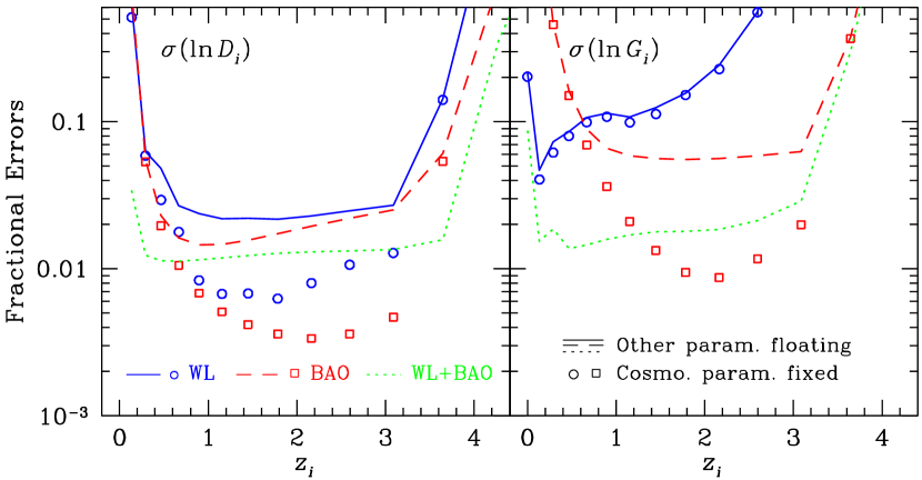
How well can LSST measure the distance and growth factor given its statistical errors? Fig. 1 presents the estimated errors on the distance (left panel) and growth (right panel) parameters from LSST WL (solid lines and open circles), BAO (dashed lines and open squares), and joint BAO and WL (dotted lines). The error of each distance (growth) parameter is marginalized over all the other parameters including the growth (distance) parameters and other distance (growth) parameters. The lines show the results with weak independent Gaussian priors on cosmological parameters: , , , and . These priors are rather weak compared to what can be achieved with Planck, except that is not constrained by CMB unless a particular cosmological model and appropriate priors are assumed. In addition, they do not introduce extra correlations between the parameters. The errors on the galaxy bias parameters (not shown) trace the errors of BAO growth parameters in this case. The symbols assume that the cosmological parameters are known precisely. A discussion on the sensitivity of these distance and growth factor constraints to individual cosmological parameters is given in Appendix A.
It is not surprising that BAO places tighter constraints on the distance parameters than WL (see also Seo & Eisenstein 2003; Song 2005; Knox et al. 2006a; Zhan & Knox 2006a, for results of either technique), but one may not expect that the former determines the growth parameters better than the latter at . It has been demonstrated that photo-z BAO measurements (without cross-bin power spectra) can constrain the combination of the galaxy bias and growth factor to several percent (Zhan & Knox 2006a), but the degeneracy between and could have left them undetermined individually. However, and are not completely degenerate here; the linear galaxy bias is treated merely as a multiplicative factor in the galaxy power spectrum, whereas the growth factor (among others) determines both the amplitude and the shape of the nonlinear matter power spectrum (Peacock & Dodds 1996). Since the BAO technique is sensitive to the shape of the power spectrum, it is able to partially break the degeneracy and constrain both and . This also means that the BAO constraints on the growth factor can be sensitive to the number of nonlinear modes included. For example, with and all the other parameters floating, the BAO error on the growth factor at in the right panel of Fig. 1 increases from to , though that at increases by only 15%. The impact of the nonlinear information is compounded by the fact that including more modes, regardless whether they are linear or nonlinear, always improves the constraints on non-degenerate parameters. If the trace term in equation (2) is roughly scale-independent, the Fisher matrix will scale as . This alone could claim a factor of 3 increase in the error as decreases from 3000 to 1000. The small difference of the errors at low redshift is due to the fact that the highest multipole there is already limited by the condition , a measure to exclude fully nonlinear modes. On the other hand, if we relax the conditions to and , the errors on the growth factor reduce to between and .
It may seem quite optimistic to rely on the nonlinear power spectrum, even if restricted to mildly nonlinear regime, for determining the growth factor. However, this is not a serious concern, because the growth factor contributes little to BAO constraints on dark energy (see Section 4.1). Moreover, it has been demonstrated that there is no significant difference between the WL dark energy constraints with a scale-free matter power spectrum or a nonlinear CDM power spectrum if the shot noise is negligible and that nonlinear evolution helps WL only because it boosts the signal on small scales where the statistical uncertainty is limited by the shot noise (ZK06b). Nevertheless, Fig. 1 suggests that the galaxy power spectra could potentially constrain dark energy and alternative gravity models with both distance and growth factor measurements as WL does if one understood the galaxy bias and nonlinear evolution well through numerical simulations (e.g., Cen & Ostriker 2000; Weinberg et al. 2004; Heitmann et al. 2005), semi-analytic modeling (e.g., Ma & Fry 2000; Peacock & Smith 2000; Croton et al. 2007), perturbative calculations (e.g., Jain & Bertschinger 1994; Jeong & Komatsu 2006), and direct measurements from higher-order statistics of the galaxy distribution (Fry 1994; Mo, Jing, & White 1997; Verde et al. 2002; Gaztañaga & Scoccimarro 2005; Sefusatti & Komatsu 2007).
The joint BAO and WL analysis reduces the errors on the distance and growth factor parameters. Although the improvement on the marginalized distance errors is moderate, the resulting constraints on the dark energy EOS parameters are much tighter than those from either technique alone (see Section 4.2). The marked improvement on the growth factor parameters is due to the fact that the shear power spectra, galaxy–shear power spectra, and galaxy power spectra have different dependencies on the galaxy bias (, , and , respectively). This further lifts the degeneracy between and , allowing significantly better determinations of .
3.3. Metric Test of Curvature
The mean curvature of the universe is of great theoretical interest. It is estimated that future large-scale BAO, SN, and WL surveys can constrain (or ) to better than with the assumption of matter dominance at and precise independent distance measurements at and at recombination (Knox 2006) or with a specific dark energy EOS (Knox et al. 2006b; Zhan 2006). However, if one assumes only the Robertson-Walker metric without invoking the dependence of the comoving distance on cosmology, then the pure metric constraint on curvature from a simple combination of BAO and WL becomes (Bernstein 2006).
Our result for from LSST WL or BAO alone is not meaningful, but the joint analysis of the two leads to with the aforementioned weak priors except that no prior is applied to . The error on changes only mildly with the number of parameters used, e.g., for 100 s and 99 s, even though errors of (the eigenmodes of) the distance and growth factor scale roughly as the square root of the number of parameters. This is expected, because the mapping between the underlying comoving distance and the observable angular diameter distance through does not depend on the number of parameters.
Planck will provide an accurate measurement of the angular diameter distance to the last scattering surface, and it can reduce the error moderately from to . Separately, the constraint weakens to with conservative estimates of systematics in photo-zs and power spectra expected for LSST (see Section 5 for more details). This is better than the forecast derived from the shear power spectra and galaxy power spectra in Bernstein (2006), because we include in our analysis more information: the galaxy–shear power spectra.
4. Probing Dark Energy with Distance and Growth Factor
With the distance and growth factor constraints from the last section, one can now answer the questions about the roles of the distance and growth factor in probing dark energy and the difference between the distance measurements from BAO and WL.
To assess the utility of distance and growth factor in constraining dark energy, we adopt a generic parametrization of the dark energy EOS and project the distance and growth factor errors onto and . We use the product of errors, , to gauge dark energy constraints, where the error is equal to that on with being held fixed (Huterer & Turner 2001; Hu & Jain 2004). This error product (EP) is proportional to the area of the error ellipse in the – plane. The figure of merit in the Dark Energy Task Force report (Albrecht et al. 2006) is the reciprocal of the product of errors on and .
4.1. Roles of Distance and Growth Factor
The relative power of the distance and growth factor in constraining the dark energy EOS has been studied in a number of ways. For example, SB05 and ZHS05 split the dark energy EOS into two constant components: that affects only the distance and that affects only the growth factor. They find that the constraints from the distance and from the growth factor are comparable. However, Knox et al. (2006a), by projecting estimated distance and growth factor errors onto a constant EOS , mention that the constraint on is due mostly to the distance. ZK06b explores this subject in yet another way; they compare the EPs with cosmological information removed from either the distance or the growth factor. Their approach is equivalent to fixing () and then projecting the errors of () onto cosmological parameter space, though they bypass the intermediate stage of estimating and errors. ZK06b shows that WL distances are much more powerful than WL growth factors in constraining and if other cosmological parameters are marginalized with weak priors and that they are comparable if the other cosmological parameters are fixed.
Because of the different methods employed, it is not straightforward to synthesize the above mentioned results. Our multi-staged approach is compatible with that in Knox et al. (2006a), and we obtain fully consistent results with those in ZK06b when their method is applied to the and errors in Section 3.2. Hence, we only need to explore the results for the method in SB05 and ZHS05.
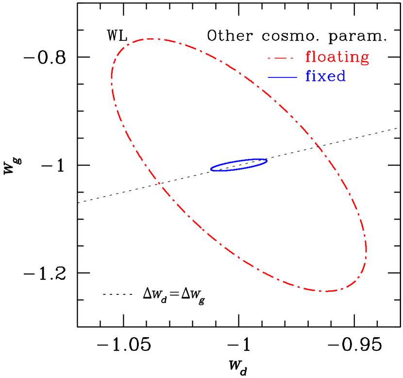
We project the WL Fisher matrix in Section 3.2 onto (, , , , , , , , , , ) using equation (3) with . The resulting error contours of and are shown in Fig. 2 with and when all the other cosmological parameters are marginalized with weak priors (dot-dashed line) and and when all the other cosmological parameters are fixed (solid line). The latter result is roughly consistent with from a single-bin shear power spectrum in SB05 and in ZHS05, though the orientation of the error contour in ZHS05 is nearly orthogonal to that in Fig. 2 and that in SB05. To examine if the differences of the assumed surveys could explain this discrepancy, we re-calculate the constraints with the survey parameters used in SB05 (, , , , , no tomography, & no redshift error). The resulting errors, and with all the other parameters fixed, and the orientation of the error contour are in good agreement with those in SB05 except that our is smaller. We are not able to reproduce Fig. 3 of ZHS05 (, , , , , , 20-bin tomography, & ); our errors on and remain positively correlated with comparable size [ & ] when all the other parameters are fixed and anti-correlated with much smaller error on [ & ] when all the other parameters are marginalized with weak priors. We note that even though Planck will place very tight constraints on CMB-related parameters, it does not have the same effect as fixing those parameters, e.g., we obtain and for LSST with Planck priors. Therefore, the distance should be at least several times more powerful than the growth factor in constraining the dark energy EOS for WL tomography.
| Probe | EP-1 | |||||
|---|---|---|---|---|---|---|
| WL | Y | Y | 0.078 | 0.22 | 0.023 | 200 |
| Y | M | 0.23 | 0.71 | 0.054 | 26 | |
| M | Y | 1.4 | 2.8 | 0.23 | 1.6 | |
| BAO | Y | Y | 0.33 | 0.81 | 0.044 | 28 |
| Y | M | 0.34 | 0.85 | 0.045 | 26 | |
| M | Y | 3.1 | 5.5 | 0.87 | 0.21 |
Note. — “Y” indicates that the set of parameters are projected onto cosmological parameter space, and “M” indicates that they are marginalized. Weak priors are applied to cosmological parameters except and , as discussed in Section 3.2. For both BAO and WL, the distance is far more powerful than the growth factor in constraining and .
The parameter splitting technique has been applied to CMB, galaxy clustering, SN, and WL data to check the consistency of dark energy models (Wang et al. 2007). The results do show that the error on is several times larger than that on , even without the galaxy clustering and SN data that provide good distance measurements at low redshift.
Another approach to isolate the roles played by the distance and growth factor is to separately marginalize distance or growth parameters and evaluate the dark energy constraints from the rest. Tables 1 (with all the other cosmological parameters floating) and 2 (with all the other cosmological parameters fixed) present such tests. There is no doubt that the growth factor is important for probing dark energy with WL tomography, as, in both tables, the EP increases by a factor of if the growth parameters are marginalized. However, given the increase of EP by a factor of when the distance parameters are marginalized, the growth factor is clearly much less constraining on the dark energy EOS than the distance.
| Probe | EP-1 | |||||
|---|---|---|---|---|---|---|
| WL | Y | Y | 0.062 | 0.15 | 0.0069 | 990 |
| Y | M | 0.12 | 0.32 | 0.029 | 110 | |
| M | Y | 0.84 | 1.8 | 0.036 | 15 | |
| BAO | Y | Y | 0.19 | 0.39 | 0.022 | 120 |
| Y | M | 0.20 | 0.42 | 0.022 | 110 | |
| M | Y | 1.3 | 2.3 | 0.072 | 6.2 |
Note. — Same as Table 1 but with all the other cosmological parameters fixed.
Tables 1 and 2 include BAO results as well. We see in both tables that the dark energy constraints are weakened by less than when the growth parameters are marginalized but more than an order of magnitude when the distance parameters are marginalized. This demonstrates that the growth factor plays almost no role in constraining and with photo-z BAO, even if it can be measured from the shape of the nonlinear power spectrum (Fig. 1).
Comparing the separate BAO and WL constraints from in Tables 1 and 2, we find that for our fiducial survey, BAO and WL achieve similar EPs (though different errors on and individually) in the absence of the growth information (and systematics). More interestingly, WL provides more information on the dark energy EOS than BAO , despite that the errors of the latter are smaller than those of the former at . The reason is that the growth factor is less sensitive to and at higher redshift and that the low-redshift growth factors, which WL measures better than BAO, are helpful in breaking the degeneracy between and (as are high-redshift distances) (Zhan 2006; ZK06b).
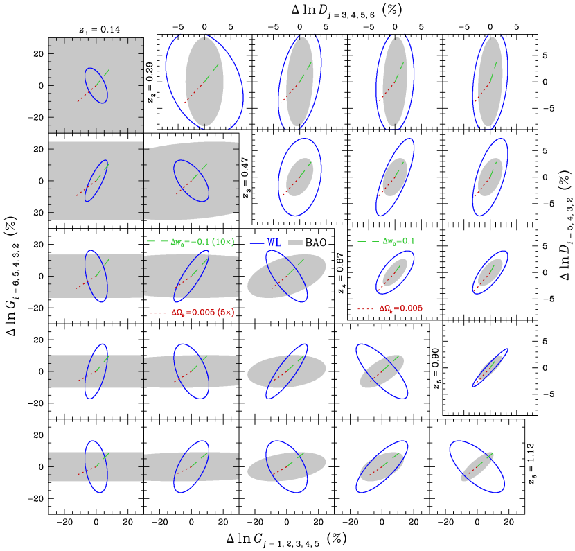
To gain a further understanding of the roles of the distance and growth factor in constraining dark energy, we show in Fig. 3 marginalized contours of – (lower triangle) and – (upper triangle) for WL (solid lines) and BAO (shaded areas). The line segments in the figure indicate the amount of change, and , due to small perturbations (dashed lines) and (dotted lines). The sensitivities of and to (not shown) are roughly and of those to , respectively. From these line segments, one can see that the sensitivity of the growth factor to and that of the distance to (and as well) decrease quickly with increasing redshift. The sensitivity of the growth factor to and has a shallow peak around .
Fig. 3 illustrates a major advantage of WL growth factors over BAO growth factors, if ever measured, in constraining the dark energy EOS: WL determines the growth factor more accurately than BAO at low redshifts where parameter sensitivities are higher. Another prominent difference between the BAO and WL constraints on the growth factor is that the WL – contours are often oriented in the most sensitive direction to the parameters, i.e., orthogonal to – caused by or , whereas the BAO ones are generally in the least sensitive direction. Therefore, one can still extract more information from the WL even when the marginalized errors of BAO are smaller. Such an advantage is seen up to beyond which the WL contours start to enclose the BAO contours completely, but the parameter sensitivities also become fairly low at .
4.2. Insights from Distance Eigenmodes
Fig. 1 and Tables 1 and 2 pose another puzzle: while the BAO distances are more accurate than the WL distances, the errors on and from the BAO distances are actually larger than those from the WL ones. ZK06b postulates that the correlation of the WL distance errors might hold the answer, but, unlike the growth factor error contours, the WL and BAO distance error contours in Fig. 3 are generally in the same direction with the former enclosing the latter. To resolve this puzzle, one has to realize that the contours in Fig. 3 are marginalized over all the other parameters including irrelevant distance and growth parameters, and useful information may have been lost in the process. To examine such information, an eigenmode analysis is needed.
Let be a distance covariance (sub-)matrix from Section 3.2. By definition, it is marginalized over all the other parameters with their priors. The distance eigenmodes satisfy
| (5) |
where is the eigenvalue corresponding to , is the number of distance parameters (remember that is replaced by ), and capitalized indices are used to avoid confusion with the indices of the distance parameters. For convenience, we sort by their eigenvalues in ascending order. Since the eigenmodes are orthonormal to each other, their covariance matrix, , is diagonal with the variance , i.e.,
| (6) |
One can interpret these as the modes of departure of the distances from the fiducial model and as a measure of how well such deviations can be determined, regardless the driving mechanism.
With equations (5) and (6), we project the marginalized distance Fisher matrix into – space
| (7) | |||||
with . We see that the contributions of the distance eigenmodes to the final Fisher matrix are separable
| (8) |
where . In other words, the – Fisher matrix consists of statistically independent contributions from the distance eigenmodes.
The number of distance parameters, , does not have much impact on the projected dark energy constraints, but it can assert artificial restrictions on these modes. Thus, before drawing conclusions from the distance eigenmodes, one must ensure that the interpolation has sufficient degrees of freedom to reflect the intrinsic properties of the distance eigenmodes of the dark energy probes, though having too many distance parameters will leave the results prone to numerical errors. Since the intrinsic eigenmodes do not vary with , one can increase until the shapes of the eigenmodes converge. In addition, the variance should grow in proportion with the degrees of freedom, , once the convergence is reached. By the same token, we change the priors on , , and to , though these priors are already too weak to make any difference.
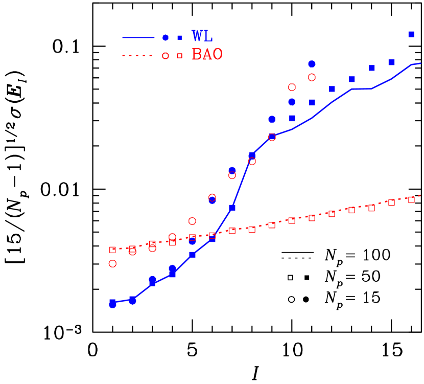
Fig. 4 shows the errors of the distance eigenmodes scaled by for WL (solid line and filled symbols) and BAO (dotted line and open symbols) with (circles), 50 (squares), and 100 (lines). The alignment between the and eigenmode errors suggests that is sufficient for the best determined modes to converge, which is confirmed upon inspection of the modes. Thereafter, we set .
An interesting result in Fig. 4 is that some WL distance eigenmodes are better determined than all the BAO distance eigenmodes, even though the marginalized errors of individual WL distance parameters are all larger than those of the BAO distance parameters in Fig. 1. This is predicted in ZK06b to be an advantage of the WL distance measurements, albeit that the best determined modes do not necessarily provide the most information on dark energy.
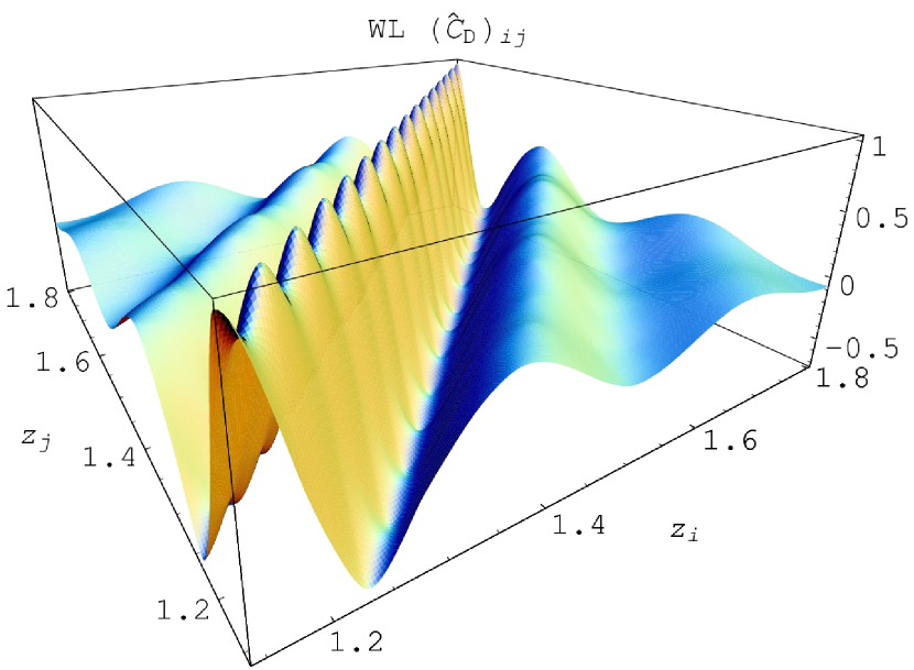
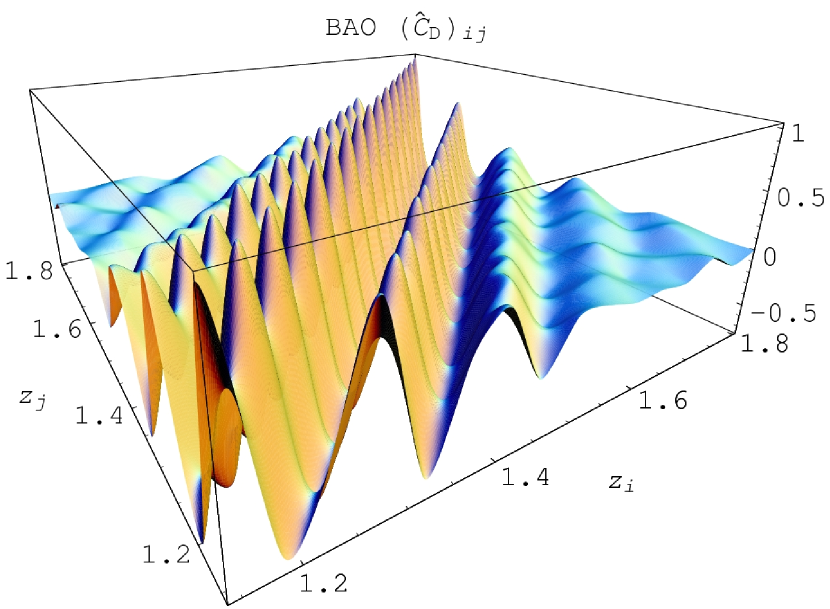
Fig. 5 shows a small piece of the distance covariance matrix of WL (left panel) and that of BAO (right panel). The covariance matrices are normalized
so that . Because the lensing kernel is much broader than the galaxy power spectrum kernel, we expect the WL distance covariance to vary more slowly than the BAO distance covariance, which is indeed seen in Fig. 5. The features of the distance covariance matrices in Fig. 5 are typical over the whole redshift range, with some broadening at both low- and high- ends, though the values of the individual covariance elements do vary with the details of the calculations such as the interpolation scheme and tomographic binning.
The characteristic difference between the distance covariance matrices of the two techniques must hold the answer to the paradox brought up at the beginning of this subsection: although BAO determines the distance more accurately than WL (the WL distance error contours also enclose the BAO ones), the EPs of each technique, when the growth parameters are marginalized, are the same with WL having smaller marginalized errors on and . Moreover, this difference also suggests that BAO and WL distance measurements are complementary.
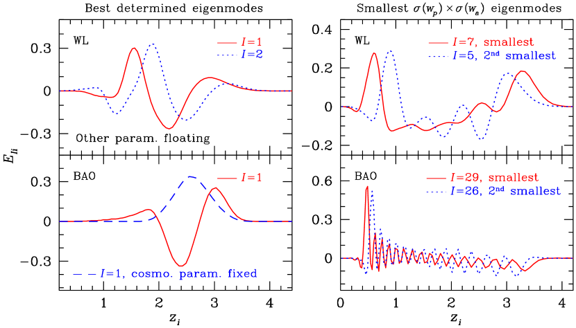
We present several eigenmodes of BAO and WL distances in Fig. 6. While not shown, the best determined WL modes (upper left panel) do not change much whether the cosmological parameters are fixed or not. These modes have close to zero mean, i.e., , and, hence, are not sensitive to the absolute normalization of the distance. To see this, assume that all the distances are subject to the same multiplicative factor (), so that the fractional errors . After projecting the distance errors on the mode , one gets the amplitude , i.e., gauges the sensitivity of an eigenmode to a change in the distance normalization. Thus the best determined WL modes show that WL is best at measuring the relative distance, which agrees with the expectation that WL tomography measures distance ratios from the lensing kernel.
The best determined BAO distance eigenmodes (lower left panel in Fig. 6) display more sensitivity to the absolute distance than the best determined WL distance eigenmodes, especially when the standard ruler of BAOs is precisely known by fixing the cosmological parameters. The best determined BAO modes peak at higher redshift than the WL ones because of the following reasons. First, the severe truncations of multipoles of the galaxy power spectra at low redshift, e.g., at vs. at , increase the low- BAO distance errors. Second, given the same source galaxy distribution, the lensing kernel peaks half-way between the observer and the source, whereas the galaxy power spectrum kernel peaks at the source. Finally, at higher redshift, the BAO features move to higher multipoles, where the smaller cosmic variance leads to better measurement of the distance.
The best determined distance eigenmodes are not necessarily the ones that contribute the most to the constraints on the dark energy EOS, because they may not be sensitive to a particular deviation of the distance–redshift relation caused by dark energy. Phrased another way, de Putter & Linder (2007) point out that the eigenmode analysis gives the expected noise of the measurements, i.e., the error of the eigenmode, but the signal, i.e., the amplitude of the mode, and the signal-to-noise ratio are not known unless comparison models are assumed (e.g., Barnard et al. 2008) or until measurements are made.
For the – parametrization of the dark energy EOS, the comparison models populate the – plane with the fiducial model (cosmological constant) at and . The contribution of each distance eigenmode to the – Fisher matrix is statistically independent of each other, so that we can evaluate the usefulness of an eigenmode by its constraint on and . Since a single mode cannot constrain both and , we apply the priors and in the projection of onto and via equation (8).
For a broad class of dark energy models, their effect on the distance is concentrated at low redshift without rapid oscillations. This means that a change of sign in at low redshift will result in a reduction of the sensitivity to the dark energy EOS. Therefore, dark-energy-efficient modes should be roughly those with a large value of at low redshift. The right column of Fig. 6 shows the distance eigenmodes with the smallest EPs for WL (upper panel) and BAO (lower panel). As expected, they all have a major peak at . The BAO modes (lower right panel) exhibit oscillatory behavior at because they are orthogonalized to other better determined modes that vary smoothly.
The fact that the best determined distance eigenmodes (with other parameters floating) from both WL and BAO are not the most sensitive modes to and means that the two dark energy probes can potentially explore a larger dark energy parameter space (e.g., Albrecht & Bernstein 2007; Barnard et al. 2008) and afford some redundancy to control certain systematic uncertainties. We also note that although and EP do not have one-to-one correspondence, contributions to the dark energy constraints naturally come mostly from the best determined modes. For WL, the dark-energy-sensitive modes are confined within , whereas for BAO, they are spread out to . This is reflected in the indices of the smallest-EP modes in Fig. 6 as well.
There has been a notion that WL tomography constrains dark energy with relative distances or distance ratios from the lensing kernel. It is true that the best determined WL distance eigenmodes are not sensitive to the normalization of the distance, but the modes that contribute the most to the constraints on and are more sensitive to the normalization of the distance. For example, the average value of of the 5 best determined WL distance eigenmodes is 0.0094, whereas that of the 5 smallest-EP modes is 1.7 (for BAO, the values are 0.033 and 1.4, respectively). Since the above results are marginalized over the growth parameters, which weakens WL’s sensitivity to the absolute distance, it is reasonable to attribute the WL constrains on dark energy to its measurements of absolute distances.
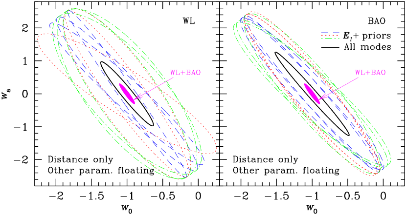
To see why the WL distances give smaller errors on and , even though they are less accurately determined than the BAO distances, we show in Fig. 7 marginalized – error contours of the eigenmodes that have the smallest EPs of each technique. The priors and are applied, and all the other parameters are marginalized with weak priors. The solid error contour in each panel shows the constraints of all 99 distance eigenmodes for each technique. Since the dark energy constraint from each eigenmode is independent of those from other eigenmodes, one can see immediately that 5 WL distance eigenmodes can account for nearly all the and constraints of WL distances. This echoes the conclusion from Fig. 6 that WL tomography has the potential of constraining more than and with all the well determined modes. Furthermore, the error ellipses of these 5 eigenmodes are oriented differently, so that they are effective in reducing the marginalized errors on and . The BAO error ellipses are narrower than the WL ones in general, but they are aligned in nearly the same direction. As such, combinations of the photo-z BAO distance eigenmodes are not effective in reducing the marginalized errors of and , and many more modes are needed to match the combined EP with that of WL (Tables 1 and 2). Because BAO and WL have different parameter degeneracy directions and because the galaxy–shear cross power spectra provide additional information, the two techniques are highly complementary to each other. Indeed, the joint BAO and WL distance constraints on and (shaded area) is roughly 9 times tighter than those from either technique alone (see also Zhan 2006).
5. Conclusions
We have disentangled the roles of the distance and growth factor in constraining the dark energy EOS and given a detailed comparison between the distance measurements from BAO and WL as well as their constraints on and . We find that if the growth parameters are marginalized without being projected onto and constraints, the EP of LSST WL will increase by a factor of . However, if the distance parameters are marginalized instead, the degradation will be two orders of magnitude. This clearly shows that the growth factor is important to WL, but the distance is far more important. In contrast, the BAO EP increases by only 10%, when the growth parameters are marginalized. It is also interesting that LSST BAO and WL achieve similar EPs when the growth parameters are marginalized.
The reconstruction of a continuous function depends on how the function is represented by discrete parameters. To explore the intrinsic properties of the reconstructed distances from BAO and WL, we assign a large number of distance and growth parameters and examine various aspects of the distance eigenmodes. This exercise leads to the finding that the WL distance eigenmodes are more complementary to each other than the BAO ones. As such, 5 WL eigenmodes can provide most of the LSST WL distance constraints on and , whereas many more are needed for BAO. A more useful result is that both LSST BAO and WL have some well determined distance eigenmodes that are not very sensitive to and . These modes may be able to constrain additional dark energy parameters and some systematic uncertainties.
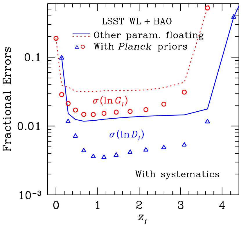
The insight gained from the results in Sections 3 and 4 in the absence of various systematics is valuable for understanding the techniques. It is also of great interest for future surveys to have more realistic error estimates that include those systematics. To this end, we present in Fig. 8 constraints on the distance (solid line and open triangles) and growth factor (dotted line and open circles) from the joint analysis of LSST BAO and WL with a conservative level of systematic uncertainties in the photo-z error distribution and additive and multiplicative errors in the shear and galaxy power spectra. The lines represent the results with other parameters floating, and the symbols are with CMB priors from Planck. By comparing with Fig. 1, one sees that the joint constraints on distance are relatively insensitive to the assumed systematics whereas those on the growth factor are affected more.
The results in Fig. 8 are marginalized over additional 30 photo-z bias parameters , 30 photo-z rms parameters , 10 shear additive error parameters , 10 shear multiplicative error parameters , and 20 galaxy additive noise parameters . We extend the additive and multiplicative shear power spectrum errors in Huterer et al. (2006) to include the galaxy power spectrum errors:
where determines how strongly the additive errors of two different bins are correlated, and and account for the scale dependence of the additive errors. Note that the multiplicative error of galaxy number density is degenerate with the galaxy clustering bias and is hence absorbed by . Below the levels of systematics future surveys aim to achieve, the most important aspect of the (shear) additive error is its amplitude (Huterer et al. 2006), so we simply fix and . For more comprehensive accounts of the above systematic uncertainties, see Huterer et al. (2006); Jain et al. (2006); Ma et al. (2006); Zhan (2006).
We have applied priors per photo-z parameter interval () in Fig. 8. For Gaussian photo-z errors with , these priors correspond to a calibration requirement of 25 spectra per redshift interval of 0.17. The constraints do not change appreciably even if one tightens the priors to , because the photo-z sample–photo-z sample cross correlations can calibrate the uncertainties in and to level (Zhan 2006). Similar results are obtained per redshift bin with spectroscopic sample–photo-z sample cross correlations (Newman 2008). For the shear multiplicative error, Massey et al. (2007) shows that current methods consistently achieve better than precision. Allowing for another 5 to 10 years of development, we are hopeful that the multiplicative errors can be controlled to half a percent, i.e., . For the shear additive error, Paulin-Henriksson et al. (2008) finds for a 15,000 deg2 ground survey that it will be well under control over relevant scales if the point spread function (PSF) is calibrated over 100 stars. LSST will be able to use on average 2 – 3 stars per square arcminute to calibrate the PSF in each exposure, so the shear additive error will not have a significant impact on scales larger than arcminute (or ) even for a single exposure. This is supported by a study with Subaru data (Wittman 2005), which shows that the correlation of the residual stellar shear after the PSF correction using only 0.9 star per square arcminute (out of arcmin-2 available) is well below the cosmic shear signal at arcminute scale for a single 10-second exposure and that it is roughly inversely proportional to the number of exposures. In addition to deep exposures in u, g, and y, LSST plans to take 400 exposures per sky field in each of its riz filters (these will be used for WL as well as photo-z). Thus it is reasonable to project that the additive shear error will be sub-dominant to the statistical errors on relevant scales. Full simulations of LSST performance are in progress. To be conservative, we assume that , which is roughly the amplitude of a shear power spectrum at . Finally, we infer from the Sloan Digital Sky Survey galaxy angular power spectrum (Tegmark et al. 2002) that the additive galaxy power spectrum error due to extinction, photometry calibration, and seeing will be at level.
With the assumed systematic uncertainties, we find that the joint analysis of LSST BAO and WL can achieve precision on 11 distances from to with weak priors on cosmological parameters. Strong priors from Planck will reduce the errors to level. The corresponding errors on the growth factors are from to without Planck and with Planck. These estimates are obtained without assuming a specific model for dark energy or modified gravity, so they are fairly model independent.
Finally, we mention that the distance and growth factor reconstruction automatically provides a pure metric measurement of the mean curvature of the universe. The joint LSST BAO and WL analysis can achieve with the above mentioned systematic uncertainties and weak priors on the other cosmological parameters. Though less impressive than other model-dependent forecasts of (Knox et al. 2006b; Zhan 2006), this estimate does not assume any specific dependence of the distance on cosmological parameters.
Appendix A Influence of Cosmological Parameters on the Distance and Growth Factor Constraints
We check the results with only one cosmological parameter fixed at a time in order to identify which ones contribute the most to the difference between the constraints with all the other parameters floating and those with all the cosmological parameters fixed in Fig. 1. For BAO distances, the matter density , the baryon density , and the curvature parameter are the most crucial parameters, and they have comparable impact on the distance errors with weighing more at higher redshift. This is expected qualitatively because and determines the standard ruler of BAOs and because the fractional difference between the comoving angular diameter distance and the comoving distance ,
is larger at higher redshift. The single most important parameter for the BAO growth factors (with galaxy bias parameters floating) is the normalization of the matter power spectrum, . The reason is that fixing removes its degeneracy with each for any single galaxy power spectrum.
The WL results are less obvious. The matter density affects the WL distance constraints the most, then the primordial spectral index , and then the normalization . Fixing these parameters reduces the uncertainty in the amplitude and shape of the matter power spectrum, which is helpful. However, the same argument applies to other parameters such as the baryon density and the running of the spectral index as well, even though and have much less impact on the distance constraints. Yet more puzzling is that the WL growth constraints hardly change whether the cosmological parameters (especially ) are fixed or not.
We do not find an intuitive explanation for the behavior of the WL distance constraints. If the derivatives of the shear power spectra with respect to two parameters are nearly degenerate, i.e., roughly proportional to each other, then the prior on one parameter will affect the constraint on the other parameter significantly. However, this is not the case; as demonstrated in the left panel of Fig. 9, none of the derivatives of the auto shear power spectrum (in the redshift bin ) with respect to , , and resemble the derivative with respect to (). Adding to the complexity is that the derivatives vary in both shape and amplitude from one power spectrum to another (right panel of Fig. 9) and that the derivative with respect to one distance parameter differs from that with respect to another distance parameter (not shown). This is true for the normalized derivatives as well.
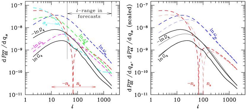
The fact that the prior on the power spectrum normalization affects the WL distance errors corroborates the conclusion in ZK06b that the WL technique measures the distance from the amplitudes of the shear power spectra. Closer inspection of equation (1) shows that also alters the amplitude of the shear power spectrum. The effect is twofold: (1) the combined factor in the window functions scales (up to a constant factor) the overdensity power spectrum to the potential power spectrum that is directly related to lensing, and (2) an increasing moves the broadband turn-over of the transfer function toward small scales, giving a small boost to the shear power spectra over the multipole range in our forecasts. This is consistent with at and, hence, the prior on having a greater impact on the WL distance constraints in Fig. 1.
In the right panel of Fig. 9, the derivatives of different shear power spectra with respect to the growth factor parameter have almost the same shape. It is likely that this characteristic sets apart the growth parameters from the rest, so that the WL growth factor constraints are practically not affected by the priors on the cosmological parameters in Fig. 1. To see why these derivatives are nearly proportional to each other, we make the approximations and
where is the interpolated growth factor, and is the Dirac delta function. We have then
| (A1) |
with showing that the redshift bins have no influence on the shape of the derivatives . Since equation (A1) does not integrate the matter power spectrum over the scales, the BAO features become visible in at in Fig. 9.
In summary, BAO measurements of the (comoving) distance are most affected by and , which determine the standard ruler of the sound horizon at the last scattering surface, and by , which relates the underlying comoving distance to the angular diameter distance. WL distance measurements are most affected by and , which effectively determine the amplitude of the lensing potential power spectrum, and by , whereas WL measurements of the growth factor do not require strong priors on cosmological parameters.
References
- Abazajian & Dodelson (2003) Abazajian, K., & Dodelson, S. 2003, Physical Review Letters, 91, 041301
- Albrecht & Bernstein (2007) Albrecht, A., & Bernstein, G. 2007, Phys. Rev. D, 75, 103003
- Albrecht et al. (2006) Albrecht, A. et al. 2006, ArXiv Astrophysics e-prints, astro-ph/0609591
- Barnard et al. (2008) Barnard, M., Abrahamse, A., Albrecht, A., Bozek, B., & Yashar, M. 2008, ArXiv e-prints, 0804.0413
- Bartelmann & Schneider (2001) Bartelmann, M., & Schneider, P. 2001, Phys. Rep., 340, 291
- Bernstein (2006) Bernstein, G. 2006, ApJ, 637, 598
- Bertschinger & Zukin (2008) Bertschinger, E., & Zukin, P. 2008, ArXiv e-prints, 0801.2431
- Blake & Glazebrook (2003) Blake, C., & Glazebrook, K. 2003, ApJ, 594, 665
- Bond & Efstathiou (1984) Bond, J. R., & Efstathiou, G. 1984, ApJ, 285, L45
- Cen & Ostriker (2000) Cen, R., & Ostriker, J. P. 2000, ApJ, 538, 83
- Chevallier & Polarski (2001) Chevallier, M., & Polarski, D. 2001, International Journal of Modern Physics D, 10, 213
- Cooray et al. (2001) Cooray, A., Hu, W., Huterer, D., & Joffre, M. 2001, ApJ, 557, L7
- Croton et al. (2007) Croton, D. J., Gao, L., & White, S. D. M. 2007, MNRAS, 374, 1303
- de Putter & Linder (2007) de Putter, R., & Linder, E. V. 2007, ArXiv e-prints, 0710.0373
- Deffayet (2001) Deffayet, C. 2001, Physics Letters B, 502, 199
- Dvali et al. (2000) Dvali, G., Gabadadze, G., & Porrati, M. 2000, Physics Letters B, 485, 208
- Eisenstein & Hu (1999) Eisenstein, D. J., & Hu, W. 1999, ApJ, 511, 5
- Eisenstein et al. (1998) Eisenstein, D. J., Hu, W., & Tegmark, M. 1998, ApJ, 504, L57
- Eisenstein et al. (2007) Eisenstein, D. J., Seo, H.-J., & White, M. 2007, ApJ, 664, 660
- Eisenstein et al. (2005) Eisenstein, D. J. et al. 2005, ApJ, 633, 560
- Fry (1994) Fry, J. N. 1994, Physical Review Letters, 73, 215
- Gaztañaga & Scoccimarro (2005) Gaztañaga, E., & Scoccimarro, R. 2005, MNRAS, 361, 824
- Guzik et al. (2007) Guzik, J., Bernstein, G., & Smith, R. E. 2007, MNRAS, 375, 1329
- Hagan et al. (2005) Hagan, B., Ma, C.-P., & Kravtsov, A. V. 2005, ApJ, 633, 537
- Heitmann et al. (2005) Heitmann, K., Ricker, P. M., Warren, M. S., & Habib, S. 2005, ApJS, 160, 28
- Holtzman (1989) Holtzman, J. A. 1989, ApJS, 71, 1
- Hu & Haiman (2003) Hu, W., & Haiman, Z. 2003, Phys. Rev. D, 68, 063004
- Hu & Jain (2004) Hu, W., & Jain, B. 2004, Phys. Rev. D, 70, 043009
- Hu & Scranton (2004) Hu, W., & Scranton, R. 2004, Phys. Rev. D, 70, 123002
- Hu & Tegmark (1999) Hu, W., & Tegmark, M. 1999, ApJ, 514, L65
- Huterer (2002) Huterer, D. 2002, Phys. Rev. D, 65, 063001
- Huterer & Takada (2005) Huterer, D., & Takada, M. 2005, Astroparticle Physics, 23, 369
- Huterer et al. (2006) Huterer, D., Takada, M., Bernstein, G., & Jain, B. 2006, MNRAS, 366, 101
- Huterer & Turner (2001) Huterer, D., & Turner, M. S. 2001, Phys. Rev. D, 64, 123527
- Ishak et al. (2006) Ishak, M., Upadhye, A., & Spergel, D. N. 2006, Phys. Rev. D, 74, 043513
- Ivezic et al. (2008) Ivezic, Z. et al. 2008, arXiv:0805.2366
- Jain & Bertschinger (1994) Jain, B., & Bertschinger, E. 1994, ApJ, 431, 495
- Jain et al. (2006) Jain, B., Jarvis, M., & Bernstein, G. 2006, Journal of Cosmology and Astro-Particle Physics, 2, 1
- Jain & Zhang (2007) Jain, B., & Zhang, P. 2007, ArXiv e-prints, 0709.2375
- Jeong & Komatsu (2006) Jeong, D., & Komatsu, E. 2006, ApJ, 651, 619
- Jing et al. (2006) Jing, Y. P., Zhang, P., Lin, W. P., Gao, L., & Springel, V. 2006, ApJ, 640, L119
- Kaiser (1992) Kaiser, N. 1992, ApJ, 388, 272
- Knox (2006) Knox, L. 2006, Phys. Rev. D, 73, 023503
- Knox et al. (2006a) Knox, L., Song, Y.-S., & Tyson, J. A. 2006a, Phys. Rev. D, 74, 023512
- Knox et al. (2006b) Knox, L., Song, Y.-S., & Zhan, H. 2006b, ApJ, 652, 857
- Linder (2003) Linder, E. V. 2003, Phys. Rev. D, 68, 083504
- Linder (2004) —. 2004, Phys. Rev. D, 70, 023511
- Lue et al. (2004) Lue, A., Scoccimarro, R., & Starkman, G. 2004, Phys. Rev. D, 69, 044005
- Ma & Fry (2000) Ma, C.-P., & Fry, J. N. 2000, ApJ, 543, 503
- Ma et al. (2006) Ma, Z., Hu, W., & Huterer, D. 2006, ApJ, 636, 21
- Massey et al. (2007) Massey, R. et al. 2007, MNRAS, 376, 13
- Mellier (1999) Mellier, Y. 1999, ARA&A, 37, 127
- Mo et al. (1997) Mo, H. J., Jing, Y. P., & White, S. D. M. 1997, MNRAS, 284, 189
- Newman (2008) Newman, J. A. 2008, ArXiv e-prints, 0805.1409
- Paulin-Henriksson et al. (2008) Paulin-Henriksson, S., Amara, A., Voigt, L., Refregier, A., & Bridle, S. L. 2008, A&A, 484, 67
- Peacock & Dodds (1996) Peacock, J. A., & Dodds, S. J. 1996, MNRAS, 280, L19
- Peacock & Smith (2000) Peacock, J. A., & Smith, R. E. 2000, MNRAS, 318, 1144
- Peebles & Yu (1970) Peebles, P. J. E., & Yu, J. T. 1970, ApJ, 162, 815
- Perlmutter et al. (1999) Perlmutter, S. et al. 1999, ApJ, 517, 565
- Refregier (2003) Refregier, A. 2003, ARA&A, 41, 645
- Riess et al. (1998) Riess, A. G. et al. 1998, AJ, 116, 1009
- Rudd et al. (2008) Rudd, D. H., Zentner, A. R., & Kravtsov, A. V. 2008, ApJ, 672, 19
- Sefusatti & Komatsu (2007) Sefusatti, E., & Komatsu, E. 2007, Phys. Rev. D, 76, 083004
- Seo & Eisenstein (2003) Seo, H., & Eisenstein, D. J. 2003, ApJ, 598, 720
- Simpson & Bridle (2005) Simpson, F., & Bridle, S. 2005, Phys. Rev. D, 71, 083501 (SB05)
- Song (2005) Song, Y.-S. 2005, Phys. Rev. D, 71, 024026
- Song & Knox (2004) Song, Y.-S., & Knox, L. 2004, Phys. Rev. D, 70, 063510
- Spergel et al. (2007) Spergel, D. N. et al. 2007, ApJS, 170, 377
- Tegmark (1997) Tegmark, M. 1997, Physical Review Letters, 79, 3806
- Tegmark et al. (2002) Tegmark, M. et al. 2002, ApJ, 571, 191
- Verde et al. (2002) Verde, L. et al. 2002, MNRAS, 335, 432
- Wang et al. (2007) Wang, S., Hui, L., May, M., & Haiman, Z. 2007, Phys. Rev. D, 76, 063503
- Weinberg et al. (2004) Weinberg, D. H., Davé, R., Katz, N., & Hernquist, L. 2004, ApJ, 601, 1
- White (2004) White, M. 2004, Astroparticle Physics, 22, 211
- White (2005) —. 2005, Astroparticle Physics, 24, 334
- Wittman (2005) Wittman, D. 2005, ApJ, 632, L5
- Wittman et al. (2000) Wittman, D. M., Tyson, J. A., Kirkman, D., Dell’Antonio, I., & Bernstein, G. 2000, Nature, 405, 143
- Zaldarriaga & Seljak (2000) Zaldarriaga, M., & Seljak, U. 2000, ApJS, 129, 431
- Zentner et al. (2008) Zentner, A. R., Rudd, D. H., & Hu, W. 2008, Phys. Rev. D, 77, 043507
- Zhan (2006) Zhan, H. 2006, Journal of Cosmology and Astro-Particle Physics, JCAP08(2006)008 (astro-ph/0605696)
- Zhan & Knox (2004) Zhan, H., & Knox, L. 2004, ApJ, 616, L75
- Zhan & Knox (2006a) —. 2006a, ApJ, 644, 663
- Zhan & Knox (2006b) —. 2006b, ArXiv Astrophysics e-prints, astro-ph/0611159 (ZK06b)
- Zhan et al. (2008) Zhan, H., Wang, L., Pinto, P., & Tyson, J. A. 2008, ApJ, 675, L1
- Zhang et al. (2005) Zhang, J., Hui, L., & Stebbins, A. 2005, ApJ, 635, 806 (ZHS05)