Ultracam photometry of eclipsing
cataclysmic variable stars
William James Feline
Department of Physics and Astronomy
The University of Sheffield
July, 2005
A thesis submitted to the University of Sheffield
in partial fulfilment of the requirements
of the degree of Doctor of Philosophy

Declaration

I declare that no part of this thesis has been accepted, or is currently being submitted, for any degree or diploma or certificate or any other qualification in this University or elsewhere.

This thesis is the result of my own work unless otherwise stated.

Summary

The accurate determination of the masses of cataclysmic variable stars is critical to our understanding of their origin, evolution and behaviour. Observations of cataclysmic variables also afford an excellent opportunity to constrain theoretical physical models of the accretion discs housed in these systems. In particular, the brightness distributions of the accretion discs of eclipsing systems can be mapped at a spatial resolution unachievable in any other astrophysical situation. This thesis addresses both of these important topics via the analysis of the light curves of six eclipsing dwarf novæ, obtained using ultracam, a novel high-speed imaging photometer.

The physical parameters of the eclipsing dwarf novæ OU Vir, XZ Eri and DV UMa are determined from timings of the white dwarf and bright spot eclipses. For XZ Eri and DV UMa the physical characteristics are also calculated using a parameterized model of the eclipse, and the results from the two techniques critically compared. This work marks the first accurate determination of the system parameters of both OU Vir and XZ Eri. The mass of the secondary star in XZ Eri is found to be close to the upper limit on the mass of a brown dwarf.

The brightness distributions of the accretion discs of the six eclipsing dwarf novæ OU Vir, XZ Eri, DV UMa, GY Cnc, IR Com and HT Cas are determined using an eclipse mapping technique. The accretion discs of the first five objects are undetected in the observations, as expected for short-period quiescent dwarf novæ with low mass transfer rates. The observations of HT Cas, however, show significant changes in the brightness distribution of the quiescent accretion disc between 2002 September and 2003 October, which are related to the overall system brightness. These differences are caused by variations both in the rate of mass transfer from the secondary star and through the accretion disc. The disc colours indicate that it is optically thin in both its inner and outer regions. I estimate the white dwarf temperature of HT Cas to be $15\,000\pm 1000$ K in 2002 and $14\,000\pm 1000$ K in 2003.

Contents

1. Declaration
2. Summary
3. Acknowledgments
4. 1 Introduction
   1. Context—
   2. 1.1 The canonical scheme
   3. 1.2 The Roche-lobe
   4. 1.3 Classification of cataclysmic variables
      1. 1.3.1 Classical and recurrent novæ
      2. 1.3.2 Dwarf novæ
      3. 1.3.3 Novalikes
      4. 1.3.4 Magnetic CVs
   5. 1.4 Cataclysmic variable evolution
      1. 1.4.1 Angular momentum loss
      2. 1.4.2 Pre-common envelope evolution
      3. 1.4.3 Common envelope evolution
      4. 1.4.4 Pre-cataclysmic variable evolution
      5. 1.4.5 Cataclysmic variable evolution
      6. 1.4.6 The orbital period distribution
      7. 1.4.7 The disrupted magnetic braking model
   6. 1.5 The gas stream and accretion disc
      1. 1.5.1 Gas stream dynamics
      2. 1.5.2 The radial temperature profile
      3. 1.5.3 Outbursts and the disc instability model
      4. 1.5.4 Superoutbursts and superhumps: SU UMa stars
      5. 1.5.5 Spiral shocks
   7. 1.6 Methods of mass determination
      1. 1.6.1 Mass-orbital period relations
      2. 1.6.2 Radial velocity mass determination
      3. 1.6.3 The photometric method of mass determination
   8. 1.7 This thesis
5. 2 Observations and data reduction
   1. 2.1 Ultracam
   2. 2.2 Journal of observations
   3. 2.3 Data reduction
      1. 2.3.1 Bias frames
      2. 2.3.2 Flat fielding
      3. 2.3.3 Dark frames
      4. 2.3.4 Extraction
      5. 2.3.5 Flux calibration
6. 3 Analysis techniques
   1. 3.1 Phasing the data
   2. 3.2 Derivative method
   3. 3.3 Lfit method
   4. 3.4 Comparing the derivative and lfit methods
   5. 3.5 Mass determination
   6. 3.6 White dwarf model atmospheres
   7. 3.7 Eclipse mapping
      1. 3.7.1 Theory
      2. 3.7.2 Practice
7. 4 OU Vir
   1. 4.1 Light curve morphology
   2. 4.2 Eclipse contact phases
   3. 4.3 Orbital ephemeris
   4. 4.4 System parameters
   5. 4.5 Eclipse mapping
8. 5 XZ Eri and DV UMa
   1. 5.1 Light curve morphology
   2. 5.2 Orbital ephemerides
   3. 5.3 Light curve decomposition
      1. 5.3.1 The derivative method
      2. 5.3.2 A parameterized model of the eclipse
      3. 5.3.3 Comparison of methods
   4. 5.4 Eclipse mapping
9. 6 GY Cnc, IR Com and HT Cas
   1. 6.1 Orbital ephemerides
   2. 6.2 GY Cnc
   3. 6.3 IR Com
   4. 6.4 HT Cas
      1. 6.4.1 Light curve morphology
      2. 6.4.2 Eclipse mapping
      3. 6.4.3 Temperature maps
10. 7 Discussion, conclusions and future work
    1. 7.1 Discussion and conclusions
       1. 7.1.1 OU Vir
       2. 7.1.2 XZ Eri and DV UMa
       3. 7.1.3 GY Cnc, IR Com and HT Cas
    2. 7.2 Overview
    3. 7.3 Future work

List of Figures

1. 1.1 An artist’s impression of a non-magnetic CV.
2. 1.2 The Cartesian co-ordinate system used throughout this thesis.
3. 1.3 Roche potentials.
4. 1.4 Types of close binary system.
5. 1.5 The ten-year light curve of SS Cyg.
6. 1.6 An artist’s impression of a polar.
7. 1.7 An artist’s impression of an intermediate polar.
8. 1.8 A schematic demonstrating the important stages in the evolution of a CV.
9. 1.9 The orbital period distribution of CVs.
10. 1.10 The trajectory of the gas stream for $q=0.15$.
11. 1.11 A sequence of eclipse maps of the dwarf nova EX Dra through the outburst cycle.
12. 1.12 The $\Sigma-T$ relation and the resulting thermal limit cycle for dwarf novæ.
13. 1.13 The superhump light distribution across the disc of Z Cha during superoutburst.
14. 1.14 The relationship between the mass ratio $q$ and orbital inclination $i$ for grazing eclipses of the bright spot and white dwarf.
15. 1.15 An eclipse of OY Car, illustrating the distinct eclipses of the white dwarf and bright spot.
16. 2.1 A ray-trace through ultracam.
17. 2.2 A CAD image of the opto-mechanical design of ultracam.
18. 2.3 A photograph of ultracam in the test focal station of the WHT just prior to commissioning on the telescope.
19. 2.4 Transmission profiles of the ultracam optical components.
20. 3.1 Phase arcs at different orbital phases.
21. 3.2 The horizontal and vertical structure of the bright spot of Z Cha and the definition of $A_{jk}$ and $Z_{jk}$.
22. 3.3 Deconvolution of the white dwarf light curve of Z Cha from the mean light curve.
23. 3.4 The model grid used to produce the fake data for comparing the results of the derivative and lfit techniques.
24. 3.5 Fake light curve produced and fitted as described in the text using the parameters given in table 3.1 for model 1.
25. 3.6 Fake light curve produced and fitted as described in the text using the parameters given in table 3.1 for model 2.
26. 3.7 Fake light curve produced and fitted as described in the text using the parameters given in table 3.1 for model 3a.
27. 3.8 Fake light curve produced and fitted as described in the text using the parameters given in table 3.1 for model 3b.
28. 3.9 Fake light curve produced and fitted as described in the text using the parameters given in table 3.1 for model 4a.
29. 3.10 Fake light curve produced and fitted as described in the text using the parameters given in table 3.1 for model 4b.
30. 3.11 Fake light curve produced and fitted as described in the text using the parameters given in table 3.1 for model 5a.
31. 3.12 Fake light curve produced and fitted as described in the text using the parameters given in table 3.1 for model 5b.
32. 3.13 Suppression of arcs in the reconstructed image.
33. 3.14 The effect of different weight functions on the default map.
34. 4.1 The light curve of OU Vir.
35. 4.2 White dwarf deconvolution of the g^′ band light curve of OU Vir of 2003 May 25.
36. 4.3 Trajectory of the gas stream from the secondary star for OU Vir.
37. 4.4 Horizontal structure of the bright spot of OU Vir.
38. 4.5 Vertical structure of the bright spot of OU Vir.
39. 4.6 Projection of the white dwarf phase arcs of OU Vir onto the plane perpendicular to the line of sight.
40. 4.7 Eclipse maps for the u^′, g^′ and i^′ 2002 May 18 light curves of OU Vir.
41. 4.8 3-dimensional plot of a blackbody fit to the reconstructed 2002 May 18 disc intensities of OU Vir.
42. 4.9 Eclipse maps for the u^′, g^′ and i^′ 2003 May 22 light curves of OU Vir.
43. 4.10 3-dimensional plot of a blackbody fit to the reconstructed 2003 May 22 disc intensities of OU Vir.
44. 5.1 The light curve of XZ Eri.
45. 5.2 The light curve of DV UMa.
46. 5.3 The $O-C$ diagram of XZ Eri produced using a linear ephemeris.
47. 5.4 The $O-C$ diagram of DV UMa produced using a linear ephemeris.
48. 5.5 The $O-C$ diagram of DV UMa produced using a quadratic ephemeris.
49. 5.6 Trajectory of the gas stream from the secondary star and the white dwarf light curve deconvolution for XZ Eri and DV UMa,.
50. 5.7 Horizontal structure of the bright spot of XZ Eri.
51. 5.8 Vertical structure of the bright spot of XZ Eri.
52. 5.9 Horizontal structure of the bright spot of DV UMa.
53. 5.10 Vertical structure of the bright spot of DV UMa.
54. 5.11 The phase-folded u^′, g^′ and r^′ light curves of XZ Eri and DV UMa as fitted by lfit.
55. 5.12 Eclipse maps for the u^′, g^′ and r^′ light curves of XZ Eri.
56. 5.13 3-dimensional plot of a blackbody fit to the reconstructed disc intensities of XZ Eri.
57. 5.14 Eclipse maps for the u^′, g^′ and i^′ light curves of DV UMa.
58. 5.15 3-dimensional plot of a blackbody fit to the reconstructed disc intensities of DV UMa.
59. 6.1 The light curves of GY Cnc, IR Com and HT Cas.
60. 6.2 The $O-C$ diagram of GY Cnc produced using a linear ephemeris.
61. 6.3 The $O-C$ diagram of IR Com produced using a linear ephemeris.
62. 6.4 The $O-C$ diagram of HT Cas produced using a linear ephemeris.
63. 6.5 The long-term light curve of HT Cas.
64. 6.6 Eclipse maps for the u^′, g^′ and i^′ 2002 September 13–14 light curves of HT Cas.
65. 6.7 Eclipse maps for the u^′, g^′ and i^′ 2003 October 29-30 light curves of HT Cas.
66. 6.8 The radial flux distribution of the reconstructed accretion disc of HT Cas for the 2002 and 2003 data.
67. 6.9 Colour-colour diagrams of the accretion disc of HT Cas in 2002 and 2003.
68. 6.10 Eclipse maps for the u^′, g^′, i^′ and z^′ light curves of GY Cnc.
69. 6.11 Eclipse maps for the u^′, g^′ and i^′ mean light curves of IR Com.
70. 6.12 3-dimensional plot of a blackbody fit to the reconstructed disc intensities of HT Cas of the 2002 data.
71. 6.13 3-dimensional plot of a blackbody fit to the reconstructed disc intensities of HT Cas of the 2003 data.
72. 7.1 The secondary star masses and orbital periods for OU Vir, XZ Eri and DV UMa, compared to two mass-period relations.
73. 7.2 The masses and radii of the secondary stars in CVs and LMXBs.

List of Tables

1. 1.1 A comparison of purely spectroscopic and purely photometric determinations of the mass ratios of selected dwarf novæ.
2. 2.1 Journal of observations.
3. 2.1 Continued. Journal of observations.
4. 2.2 Determination of zero-points from ultracam SDSS standard stars.
5. 3.1 The input parameters of the fake light curves used for comparison of the derivative and lfit methods.
6. 3.2 Reconstructed parameters from lfit.
7. 3.2 Continued. Reconstructed parameters from lfit.
8. 3.3 Reconstructed parameters from the derivative method.
9. 3.3 Continued. Reconstructed parameters from the derivative method.
10. 3.4 Prescriptions for weight functions $\omega_{jk}$.
11. 3.5 The parameters used in the maximum entropy reconstructions of the disc intensities.
12. 4.1 Mid-eclipse timings of OU Vir.
13. 4.2 White dwarf contact phases and flux of OU Vir.
14. 4.4 Mean position and extent of the bright spot of OU Vir.
15. 4.5 System parameters of OU Vir.
16. 5.1 Mid-eclipse timings of XZ Eri and DV UMa.
17. 5.2 White dwarf contact phases and out-of-eclipse white dwarf fluxes of XZ Eri and DV UMa.
18. 5.3 Bright spot contact phases of XZ Eri and DV UMa.
19. 5.4 Mean position and extent of the bright spots of XZ Eri and DV UMa.
20. 5.5 Parameters of XZ Eri fitted using lfit.
21. 5.6 Parameters of DV UMa fitted using lfit.
22. 5.7 System parameters of XZ Eri and DV UMa derived using the Nauenberg mass–radius relation.
23. 6.1 Mid-eclipse timings of GY Cnc, IR Com and HT Cas.
24. 6.2 White dwarf contact phases of IR Com.

Chapter 1 Introduction

Context—

“On the evening of December 15th, 1855, I remarked …an object shining as a star of the ninth magnitude, with a very blue planetary light, which I have never seen before during the five years that my attention has been directed to this quarter of the heavens. On the next fine night, Dec. 18th, it was certainly fainter than on the 15th by half a magnitude or more. Since that date I have not had an opportunity of examining it till last evening, January 10th, when its brightness was not greater than that of stars of the twelfth magnitude.”

This description, by J. R. Hind (1856), marked the discovery of a new class of variable star—the dwarf novæ. The star was soon christened U Geminorium, and in subsequent years became an exemplar of its type. Significantly, Hind noted that the object appeared very blue, implying high temperatures, which differentiated it from other variables such as Algol (an eclipsing binary) and S Cancri (a Mira variable). Furthermore, U Gem varied seemingly at random, a fact later bemoaned by Parkhurst (1897): “Predictions with regard to it can better be made after the fact.”

The U Gem stars eventually became known as dwarf novæ (Payne-Gaposchkin & Gaposchkin, 1938), by comparison to the even more spectacular novæ which have been observed since antiquity, and are now called classical, or old, novæ. These objects now form part of the group of stars referred to as the cataclysmic variables.

The currently accepted model of cataclysmic variables was originally developed by Kraft (1959, 1962), who proposed that

“…all members of this group are spectroscopic binaries of short period. …the blue stars in these systems are probably white dwarfs. The masses of the red components and their spectra …seem consistent with a star of mass $\sim 1\;{\rm M}_{\odot}$. …the red stars overflow their lobes of the inner Lagrangian surface; the ejected material forms, in part, a ring, or disc, surrounding the blue star.”

This model has subsequently been expanded on (Warner & Nather, 1971; Smak, 1971), but remains essentially valid. In fact, any system which fits this description can accurately be described as a cataclysmic variable.

1.1 The canonical scheme

Cataclysmic variable stars (CVs) are semi-detached binary systems, with orbital periods of a few hours. The secondary star (of mass $M_{2}$), usually a main-sequence star, transfers material to the white dwarf primary (of mass $M_{1}$). In non-magnetic systems (in which the magnetic field of the white dwarf is too weak to affect the accretion flow), the material is transferred via a gas stream, and then spirals round the primary star, forming an accretion disc. The collision of the gas stream with the accretion disc forms a so-called ‘bright spot,’ a shock-heated region of emission at the edge of the disc. At the inner edge of the accretion disc, the disc material, orbiting in Keplerian orbits, is decelerated to match the surface velocity of the white dwarf in a boundary layer. If the white dwarf has a significant magnetic field, however, the disc and boundary layer can be partially (in the case of intermediate polars) or totally (in the case of polars) disrupted and the accreting material instead flows along magnetic field lines onto the surface of the primary star (see § 1.3.4). Figure 1.1 shows an artist’s impression of a non-magnetic CV, with the main features labelled.

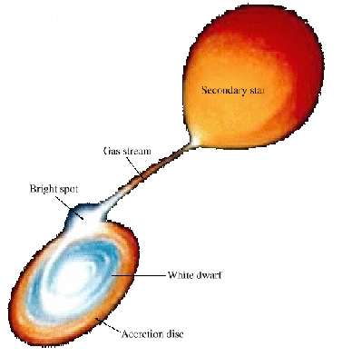
Figure 1.1: An artist’s impression of a non-magnetic CV, with the red dwarf secondary, gas stream, accretion disc and white dwarf primary marked.

The name cataclysmic comes from the violent but non-destructive outbursts that first drew attention to these objects (see § 1.3.1). These periodic outbursts mean that monitoring of CVs is a popular and fruitful task among many amateur astronomers.

In systems which are inclined at large angles to our line of sight ($i\gtrsim 70^{\circ}$), eclipses of the various components occur, which can lead to fine structure in the eclipse morphology. Eclipses of the white dwarf and bright spot are sharp (of the order of tens of seconds), due to the compact nature of these regions, and are superimposed on the more gradual eclipse of the extended accretion disc. As the bright spot rotates into view, it can give rise to an increase in the observed flux, resulting in an ‘orbital hump’ in the light curve.

1.2 The Roche-lobe

The orbital separation $a$ of the binary components is, from Newton’s form of Kepler’s third law, a function of the mass of each component and the orbital period, $P_{\rm{orb}}$:

$$a^{3}=\frac{(M_{1}+M_{2})GP^{2}_{\rm{orb}}}{4\pi^{2}},$$ (1.1)

where $G$ is the gravitational constant. Given that the masses of the stellar components of CVs are approximately solar, and that the orbital periods are of the order a few hours, equation 1.1 implies binary separations of the order of one solar radius.

Such short orbital periods and close proximity mean that tidal forces from the gravitational field of the primary and centrifugal forces from the rotation cause the secondary star in CVs to be distorted into a teardrop shape from the spherical shape that an isolated star would assume. These tidal forces also ensure that the secondary is tidally locked: it rotates at the same rate as it orbits. The time-scale for synchronization is short, as material flowing into and out of the tidal bulge will obviously expend a great deal of energy in doing so. In contrast, the small radius of the primary means that it remains effectively immune from such forces and its shape remains spherical.

Before going into the details of the Roche geometry, I first define a co-ordinate system to use. As is usual, I use a set of right-handed Cartesian co-ordinates, with the x-axis being defined as the line joining the centres of the two stars; the y-axis is in the orbital plane, perpendicular to the x-axis and in the direction of orbital motion; and the z-axis is perpendicular to the binary plane. This co-ordinate system is illustrated in figure 1.2.

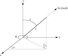
Figure 1.2: The Cartesian co-ordinate system used throughout this thesis. The frame is co-rotating with the binary system, with the primary star at the origin. The x-axis is the line joining the centres of the two stars, with x increasing towards the secondary; the y-axis is in the binary plane, perpendicular to the x-axis and in the direction of orbital motion; and the z-axis is perpendicular to the binary plane. $i$ denotes the orbital inclination, $\phi$ the orbital phase and $\rm{r}$ is the length of the vector pointing towards Earth.

The total potential of the system is given by the sum of the gravitational potentials of the two stars and the effective potential of the centrifugal force. In the above co-ordinate system, the total potential is therefore (Kruszewski, 1966; Pringle, 1985; Frank, King, & Raine, 1985)

$$\Phi=-\frac{GM_{1}}{aR_{1}}-\frac{GM_{2}}{aR_{2}}-\frac{2\pi^{2}a^{2}}{P^{2}_{\rm orb}}\left[\left(x-\frac{M_{2}}{M_{1}+M_{2}}\right)^{2}+y^{2}\right],$$ (1.2)

where $R_{1}$ and $R_{2}$ are the distances from the relevant star and $y$ and $x$ are the distances along the relevant axes, all in units of the orbital separation $a$.

Contours of equal potential, $\Phi=$ const, are known as Roche equipotentials. The shapes of these equipotentials are functions only of the mass ratio $q=M_{2}/M_{1}$, and their scale depends on the orbital separation. The Lagrangian points 1–5 (${\rm L}_{1}\ldots{\rm L}_{5}$), first discovered in 1772 by Lagrange, satisfy

$$\frac{\partial\Phi}{\partial(x,y,z)}=0,$$ (1.3)

so a test particle at a Lagrangian point experiences no net force. As figure 1.3 illustrates, this is an unstable equilibrium, as the Lagrangian points are potential maxima.

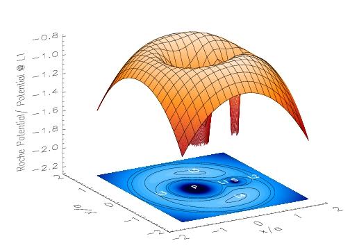
Figure 1.3: Different representations of the Roche potential. The potential scale is normalised such that the potential at the ${\rm L}_{1}$ point is $-1.0$. The orange surface is a ‘rubber-sheet’ representation of the Roche potential. The two deep depressions correspond to the two stars. This surface is colour–coded: darker colours indicate a more negative potential. The black grid superimposed on this surface shows the potential on lines of equal x- and y-values. The blue plane below this shows the same potential, but in two dimensions. The black curves superimposed on this plane are Roche equipotentials. The ‘critical potential’ on which the ${\rm L}_{1}$ point lies is one of them (the figure of eight). All the Lagrangian points are marked, as are the positions of the primary and secondary stars. The mass ratio $q$ is 0.175 and the orbital period is 1.74 hours.

The largest closed equipotentials of each component meet at the inner Lagrangian point ${\rm L}_{1}$ (see figure 1.3). The surface defined for each component by this equipotential is called the Roche-lobe of that star; the potential defining the Roche-lobe is known as the critical potential. Once the Roche-lobe is filled, equation 1.3 shows that the material at the ${\rm L}_{1}$ point can easily transfer to the other star (see § 1.5.1), with the initial impetus being given by the gas pressure of the secondary star’s atmosphere.

It is frequently useful to use the volume radius of the Roche-lobe $R_{\rm{L}}$ as a measure of the size of the secondary. This is defined as the radius of the sphere that would have the same volume as the Roche-lobe (Eggleton, 1983):

$$R_{\rm{L}}=\frac{0.49aq^{\frac{2}{3}}}{0.6q^{\frac{2}{3}}+\ln\left(1+q^{\frac{1}{3}}\right)}\,, 0<q<\infty$$ (1.4)

which is accurate to better than 1 per cent.

I have previously stated that CVs are ‘semi-detached binary systems.’ These are a sub-type of binary stars known collectively as ‘close binary systems.’ The defining characteristic of close binary stars is the presence of an interaction between the two components other than that of gravity. Alternatively and equivalently, close binaries can be defined as systems in which the two stars affect each others’ evolution. This interaction can take the form of irradiation of one star by the other, or as in the case of CVs, mass being transferred from one star to the other. Close binaries come in three flavours, illustrated in figure 1.4: detached binaries have both stellar components contained within their respective Roche-lobes; semi-detached binary stars (including all CVs) have only one component within its Roche lobe, the other fills its Roche-lobe and can transfer mass to the detached star; in the case of contact binaries both stars overfill their Roche-lobes.

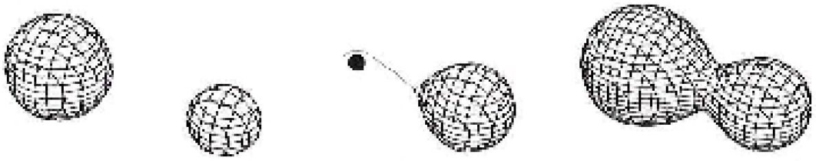
Figure 1.4: Different types of close binary systems. From left: detached binaries have both components within their Roche-lobes (e.g. NN Ser); semi-detached binaries (including all CVs) have only one component within its Roche-lobe, the other fills its Roche-lobe and can transfer mass to the detached star; in contact binaries both stars overfill their Roche-lobes (e.g. W UMa stars). From Hellier (2001).

1.3 Classification of cataclysmic variables

The classification of CVs is rooted in the historical observations of these objects, which concentrated, for obvious reasons, on the spectacular outbursts that characterise these stars and lend them their name. The amplitude and duration of outbursts were obvious parameters by which to classify CVs in the past, and by-and-large remain so today.

1.3.1 Classical and recurrent novæ

The novæ that first drew the eye to CVs are dramatic increases in brightness of these stars. The amplitude of these eruptions ranges between 6 and $\sim 19$ magnitudes, and last for a few days to years. These eruptions are of such magnitude that to ancient astronomers they appeared to be new stars. Ancient Chinese astronomers dubbed them ‘guest stars,’ whereas in the West they became known as novæ stella.

Classical novæ have by definition only been observed to go nova once. These are further subdivided on the basis of their duration into fast novæ and slow novæ (which can last for years). The nova duration is strongly correlated with the eruption amplitude—the fastest novæ also have the greatest amplitudes.

Recurrent novæ are classical novæ that have been observed to erupt more than once. The lack of definite novæ recurrences from historical records (Duerbeck, 1992) implies that, in general, the recurrence time is $>1000$ years (Warner, 1995, page 258). The ejection, at high velocity, of a substantial shell from recurrent novæ permits them to be distinguished from dwarf novæ which do not emit such a shell. (Dwarf novæ may, however, have an enhanced stellar wind during outburst.)

The nova eruption is thought to be due to the accumulation of hydrogen-rich material from the accretion disc on the surface of the white dwarf. As material is accumulated, the temperature and density of this layer eventually become high enough for nuclear reactions to occur. Since the accreted material is degenerate, the pressure is independent of temperature and a thermonuclear runaway occurs in the accreted layer of hydrogen (the white dwarf itself is mainly composed of carbon and oxygen). An exponential increase in energy generation, the nova eruption, occurs until the Fermi temperature is reached, and the degeneracy is lifted.

1.3.2 Dwarf novæ

The outbursts (discussed in more detail in § 1.5.3) that characterise dwarf novæ are rather less in amplitude (typically between two and five magnitudes) than those of novæ, hence the term dwarf novæ. Outbursts typically last for about a week, with the interval between outbursts (which varies from ten days to many years) being correlated with their duration. Both the amplitude and duration of an outburst have well defined time-scales for a particular object. The light curve of SS Cyg, the brightest and one of the best-studied dwarf novæ, is shown in figure 1.5, over a period of ten years.

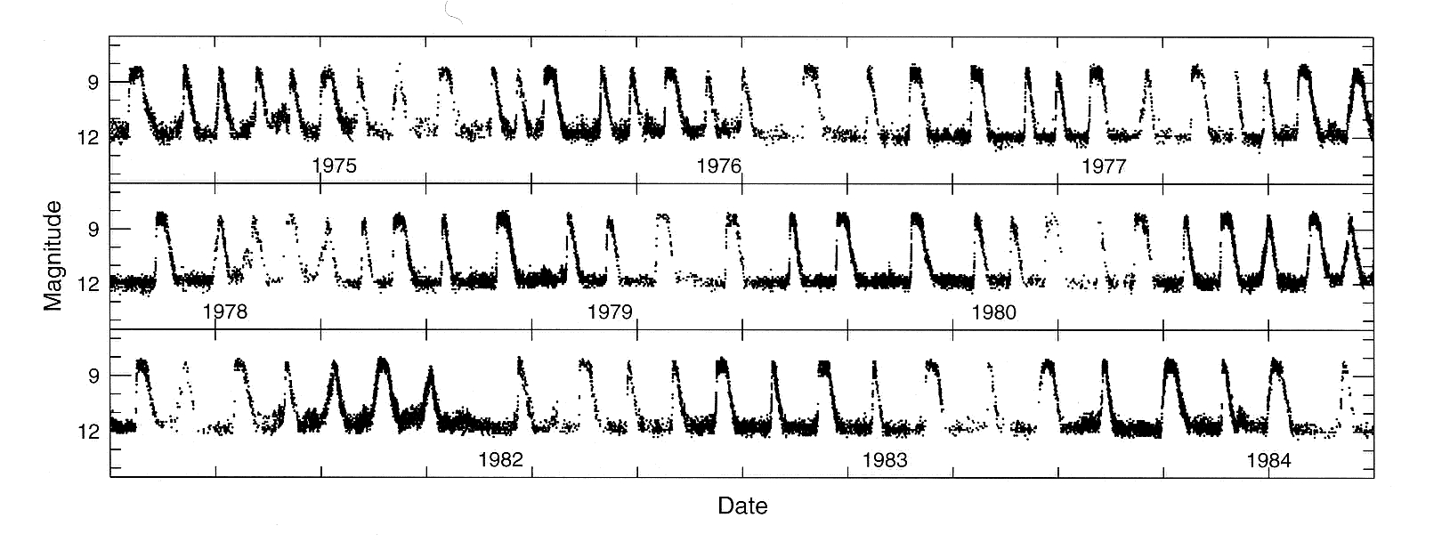
Figure 1.5: The ten-year light curve of SS Cyg, showing regular outbursts. Compiled by the American Association of Variable Star Observers (AAVSO), and reproduced from Hellier (2001). Tick-marks are at 100 day intervals.

There exist three distinct subtypes of dwarf novæ:

1. Z Cam stars have light curves that show periods of rapid outburst activity interspersed with standstills, periods of constant brightness about 0.7 magnitudes below maximum light. These standstills last between tens of days and years. It is believed that Z Cam stars have mass transfer rates close to that required to maintain the disc in permanent outburst, with occasional changes in the rate of mass transfer from the secondary star causing the onset of outbursts and subsequent return to standstill.

2. SU UMa stars exhibit superoutbursts in addition to regular outbursts (see § 1.5.4). These superoutbursts are approximately 0.7 magnitudes brighter than normal outbursts, of longer duration and somewhat more regular. They often appear to be triggered by normal outbursts, as a pause before maximum superoutburst brightness is achieved reveals (Warner, 1995, page 188).

   SU UMa stars have another unique characteristic of their light curves—the superhump. These are periodic humps in the light curves of dwarf novæ near the maximum of superoutburst. Superhumps have periods of a few percent longer than the orbital cycle, and their amplitude appears to be independent of the orbital inclination. SU UMa stars are discussed in more detail in § 1.5.4.

3. U Gem stars are the dwarf novæ that are neither Z Cam nor SU UMa stars.

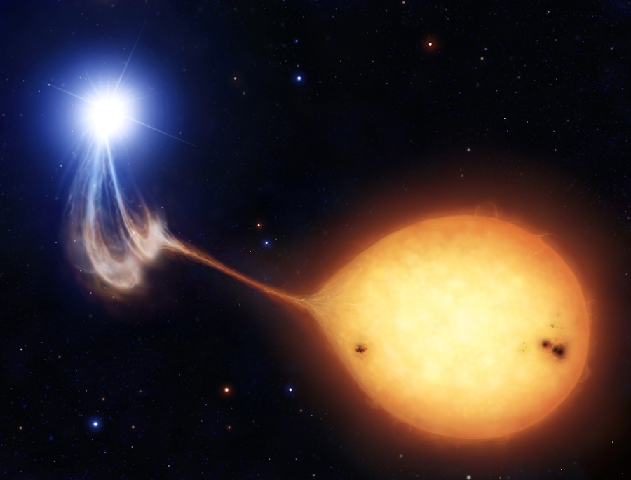
Figure 1.6: An artist’s impression of a polar. Image used by the kind permission of Mark A. Garlick.

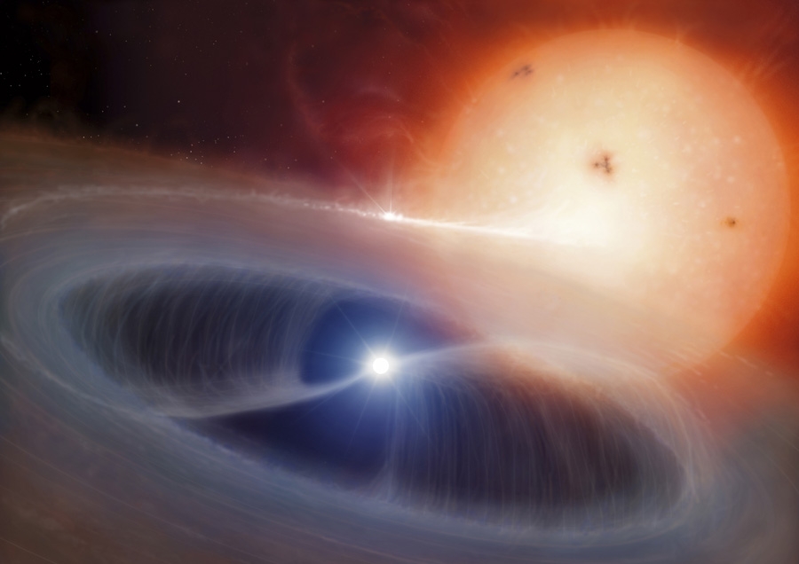
Figure 1.7: An artist’s impression of an intermediate polar. Image used by the kind permission of Mark A. Garlick.

1.3.3 Novalikes

Historically, nova-like variables were classified as such because they were observed to be spectroscopically similar to the remnants of old novæ, but had not been observed (yet) to undergo a nova eruption. Old novæ are also classed as novalikes, and the category contains all CVs with mass transfer rates sufficiently high to maintain the disc in permanent outburst (see § 1.5.3).

1.3.4 Magnetic CVs

If the white dwarf has a strong magnetic field the accretion process can be significantly affected. Depending on the strength of the field, the gas stream and accretion disc can be partially or totally disrupted.

Polars, otherwise known as AM Her stars, are those CVs with the strongest magnetic fields (typically a few tens of MGauss). The magnetic field of the primary is so strong that the white dwarf’s rotation is tidally locked to the orbital period (i.e. the primary is phase-locked or rotates synchronously) and the gas stream is disrupted, splitting in two and flowing along the magnetic field lines to the white dwarf (figure 1.6). Synchronous rotation (at least in the long-term; nova eruptions can temporarily knock the system out of synchronization) is the defining characteristic of polars.

Intermediate polars have significant magnetic fields that are not strong enough to entirely disrupt the accretion process. If the field is of such a strength that the gas stream becomes attached to the field lines at a radius greater than the minimum circularisation radius (Verbunt & Rappaport, 1988; see § 1.5.1) then a disc cannot form. If the field is weaker and material begins to follow the field lines within this radius, then a truncated disc structure is formed instead (figure 1.7).

Intermediate polars and polars may be observationally distinguished due to asynchronous rotation of the white dwarf manifesting itself in the form of periodicities in the light curves of intermediate polars.

1.4 Cataclysmic variable evolution

Single star evolutionary theory predicts that white dwarfs form from the cores of red giant stars. The radii of red giants are typically between 50 to 500 R_⊙. How then do we reconcile the orbital separations found in typical CVs of approximately 1 $R_{\odot}$ with the giant progenitor stars of CVs? The answer is that the orbital separations of CVs shrink over their lifetime as they evolve, from initial separations greater than the radii of their progenitor stars to the separations that we observe today. Proper consideration of the effects of angular momentum is crucial to a complete understanding of many stages of CV evolution, so I begin this section with a discussion of the mechanisms of angular momentum loss in CVs.

1.4.1 Angular momentum loss

The total orbital angular momentum of the system $J$ is given by

$$J=M_{1}a_{1}\frac{2\pi a_{1}}{P_{\rm{orb}}}+M_{2}a_{2}\frac{2\pi a_{2}}{P_{\rm{orb}}},$$ (1.5)

where $a_{1}$ and $a_{2}$ are the distances of the primary and secondary stars, respectively, from the centre of mass of the system. Since $a=a_{1}+a_{2}$, $M=M_{1}+M_{2}$ and $a_{1}M_{1}=a_{2}M_{2}$, using Kepler’s third law (equation 1.1) leads to

$$J=M_{1}M_{2}\left(\frac{Ga}{M}\right)^{\frac{1}{2}}.$$ (1.6)

Differentiating equation 1.6 logarithmically with respect to time and assuming that no mass is lost from the system as a whole (i.e. $\dot{M}=0$) gives

$$\frac{\dot{a}}{a}=2\frac{\dot{J}}{J}-2\frac{\dot{M}_{2}}{M_{2}}\left(1-\frac{M_{2}}{M_{1}}\right),$$ (1.7)

where the dot indicates the rate of change with respect to time (i.e. $\dot{M_{2}}$ is the secondary’s rate of change of mass).

The above expression gives the response of the orbital separation to mass transfer and angular momentum loss. One can use the approximate relation of Paczyński (1971) for the volume radius of the Roche lobe

$$R_{\rm{L}}=0.462a\left(\frac{M_{2}}{M}\right)^{\frac{1}{3}}, 0<q<0.3$$ (1.8)

which is accurate to 2 per cent, with equation 1.7 to derive a similar expression for the response of the Roche-lobe: logarithmically differentiating equation 1.8 and combining with equation 1.7 gives

$$\frac{\dot{R}_{\rm{L}}}{R_{\rm{L}}}=2\frac{\dot{J}}{J}+\left(2\frac{M_{2}}{M_{1}}-\frac{5}{3}\right)\frac{\dot{M}_{2}}{M_{2}}.$$ (1.9)

The above is equally valid if the usual rôles of the primary and secondary stars are reversed, that is, if the primary is the component losing mass. The relevant subscripts in equations 1.5–1.9 merely need to be reversed (i.e. $M_{2}\rightarrow M_{1}$ etcetera).

Angular momentum loss in CVs is believed to occur via two main mechanisms: magnetic braking and gravitational radiation.

Magnetic braking

The two essential components of magnetic braking are an ionized stellar wind and a stellar magnetic field. We expect (Basri, 1987) both of these to occur for the secondary stars of CVs.

The ionized stellar wind from the secondary is forced to co-rotate with the star due to coupling with the magnetic field lines. The stellar wind thus exerts a braking torque on the rotation of the secondary star. As tidal forces keep the secondary’s rotation synchronous with the orbital motion, the energy effectively comes from the orbital motion. The orbital separation therefore shrinks due to the loss of angular momentum to the stellar wind.

The standard picture of CV evolution (Rappaport et al., 1983) has magnetic braking as the main source of angular momentum loss until the secondary star becomes fully convective, whereupon angular momentum loss due to magnetic braking ceases (see also § 1.4.7). However, Andronov et al. (2003) showed that if the angular momentum loss properties of the secondary stars in CVs are identical to those of single (or detached binary) stars (Basri, 1987), then the time-scale for angular momentum loss due to magnetic braking is two orders of magnitude greater than for the ‘standard’ model. This implies a much longer evolutionary time-scale for CVs. The data used by Basri (1987), however, only includes systems with orbital periods $\gtrsim 17$ hr: it is not clear that the results can be extrapolated to systems with shorter periods such as most CVs. In a recent paper, Andronov & Pinsonneault (2004) found that chemical evolution of the secondary star affects its angular momentum loss properties. The result is that the angular momentum loss rate in CV secondaries may be greater than that of single stars, although it is still predicted to be significantly less than in the standard picture. The exact form of the angular momentum loss due to magnetic braking remains uncertain.

Gravitation radiation

The small orbital separation of many CVs makes gravitational radiation a significant source of angular momentum loss for these systems. The rate of the angular momentum loss $\dot{J}$ is given by (Landau & Lifschitz, 1958)

$$\frac{\dot{J}}{J}=-\frac{32G^{3}}{5c^{5}}\frac{M_{1}M_{2}(M_{1}+M_{2})}{a^{4}}.$$ (1.10)

Gravitational radiation may be the dominant mechanism for some short-period dwarf novæ and polars (Warner, 1995, page 447). Observations of orbital period decay in binary pulsars (e.g. PSR 1913+16; Taylor & Weisberg, 1982) has provided convincing observational evidence for the existence of gravitational radiation.

1.4.2 Pre-common envelope evolution

The progenitor stars of CVs stars start life as members of a wide binary system. The more massive member of the binary naturally evolves to the red giant phase more rapidly, expands to fill its Roche-lobe and mass transfer (from the primary to the secondary star) begins. Mass is being transferred farther from the centre of mass, and so in order to conserve angular momentum (i.e. $\dot{J}=0$), the orbital separation decreases (equation 1.7) and the Roche-lobe shrinks in size (equation 1.9).

The radius of a giant star is almost entirely governed by the mass of its degenerate core; it does not depend on the mass of its outer atmosphere. It follows that mass transfer from the primary to the secondary star is unstable, as no stabilising reduction in radius of the mass donor occurs. Mass transfer proceeds on the dynamical time scale (Warner, 1995, page 450): $\dot{M}\sim M/\tau_{\rm{dyn}}$, where

$$\tau_{\rm{dyn}}\sim\left(\frac{R^{3}}{GM}\right)^{\frac{1}{2}}.$$ (1.11)

However, the mass-receiving star can only adjust its structure on the thermal, or Kelvin-Helmholtz time scale (Warner, 1995, page 450):

$$\tau_{\rm{KH}}=\frac{GM^{2}}{RL}\gg\tau_{\rm{dyn}},$$ (1.12)

where $L$ is the stellar luminosity. The end result is runaway mass transfer leading to the transferred material forming an extended common envelope around both stars.

1.4.3 Common envelope evolution

The common envelope phase of CV evolution is when the vast majority of the orbital separation shrinkage in CVs occurs. The pre-CV is effectively orbiting within the atmosphere of a red giant. The drag the stars encounter within the common envelope results in orbital angular momentum being deposited within the envelope. The consequent loss of energy from the orbit shrinks the binary separation to $\sim 1\;{\rm R}_{\odot}$ in approximately 1000 years. The energy injected into the common envelope causes it to be ejected as a planetary nebula, revealing a still-detached pre-cataclysmic star consisting of a white dwarf primary and a red dwarf secondary star.

1.4.4 Pre-cataclysmic variable evolution

Evolution into contact and the formation of a CV occur due to angular momentum loss from the system. Equation 1.9 illustrates that for zero angular momentum loss ($\dot{J}=0$) the minimum radius of the secondary’s Roche-lobe occurs for $q=5/6$. Despite this, mass transfer clearly occurs in CVs, most of which have $q<5/6$. To drive mass transfer hence requires the loss of angular momentum from the system ($\dot{J}<0$).

For pre-CVs, magnetic braking is by far the most significant source of angular momentum loss. For the more massive secondary stars with $M_{2}\gtrsim 1\;{\rm M}_{\odot}$, evolution of the secondary and consequent expansion may cause it to come into contact with its Roche-lobe before angular momentum loss does. Pylyser & Savonije (1988a, b) found that contact due to evolution of the secondary star leads to mass transfer driven by expansion of the secondary’s envelope, an increasing orbital period (and separation) and, ultimately, a detached system (occurring when all the secondary’s envelope has been lost). In this thesis, I concentrate on the more common (as for most CV secondaries $M_{2}\ll 1\;{\rm M}_{\odot}$) scenario of angular momentum loss.

1.4.5 Cataclysmic variable evolution

The evolution of CVs relies on mechanisms of angular momentum loss in order to drive mass transfer. In the case of CVs, mass transfer occurs from the secondary star to the primary. Mass is therefore moving away from the centre of mass and from equations 1.7 and 1.9 if angular momentum is conserved ($\dot{J}=0$), for $q<5/6$ (i.e. most CVs), this results in the orbital separation and volume radius of the secondary’s Roche-lobe increasing, cutting off mass transfer. A mechanism of angular momentum loss ($\dot{J}<0$) is therefore necessary for long-term mass transfer to occur. Mass transfer through angular momentum loss must lead to the volume radius of the secondary star’s Roche-lobe and the orbital separation shrinking, resulting (equation 1.1) in the system evolving to shorter orbital periods.

For mass transfer to be stable, the secondary must be able to adjust its radius quickly enough to remain within its Roche-lobe, i.e. (Warner, 1995, page 458)

$$\xi=\frac{\partial\ln R_{2}}{\partial\ln M_{2}}>\frac{d\ln R_{L}}{d\ln M_{2}}.$$ (1.13)

Equations 1.9 and 1.13, for conservative mass transfer ($\dot{J}=0$), require

$$q<\frac{1}{2}\xi+\frac{5}{6}$$ (1.14)

for stable mass transfer to occur. For $M_{2}>M_{\odot}$, where $\tau_{{\rm KH}}<\tau{{}_{\rm ML}}$ (where $\tau{{}_{\rm ML}}$ is the time scale for mass loss) $\xi=0.87$ (Warner, 1995, page 458), this leads to the condition $q<1.26$ for mass transfer from a main-sequence donor star to be stable. For $M_{2}>0.8\;M_{\odot}$, $\tau_{{\rm KH}}>\tau{{}_{\rm ML}}$ and $\xi=-1/3$ (Paczyński, 1965), the corresponding condition is $q<2/3$. If this condition is not satisfied (in either case) then mass transfer is unstable and will proceed on the dynamical time-scale (equation 1.11), possibly leading to a second common envelope phase.

It is easiest to think of the secular evolution of CVs as occurring in a stepwise way (although the process is of course continuous in practice). First, mass is transferred from the secondary star to the primary. This causes, through equations 1.7 and 1.9, the orbital separation and secondary star’s Roche-lobe to increase in size. The radius of the secondary star becomes smaller in response to its reduced mass. Angular momentum loss from the system then decreases both the orbital separation and the size of the secondary star’s Roche-lobe until mass transfer can re-commence at a smaller orbital separation than previously.

A schematic demonstrating the important stages in the evolution of a CV is shown in figure 1.8.

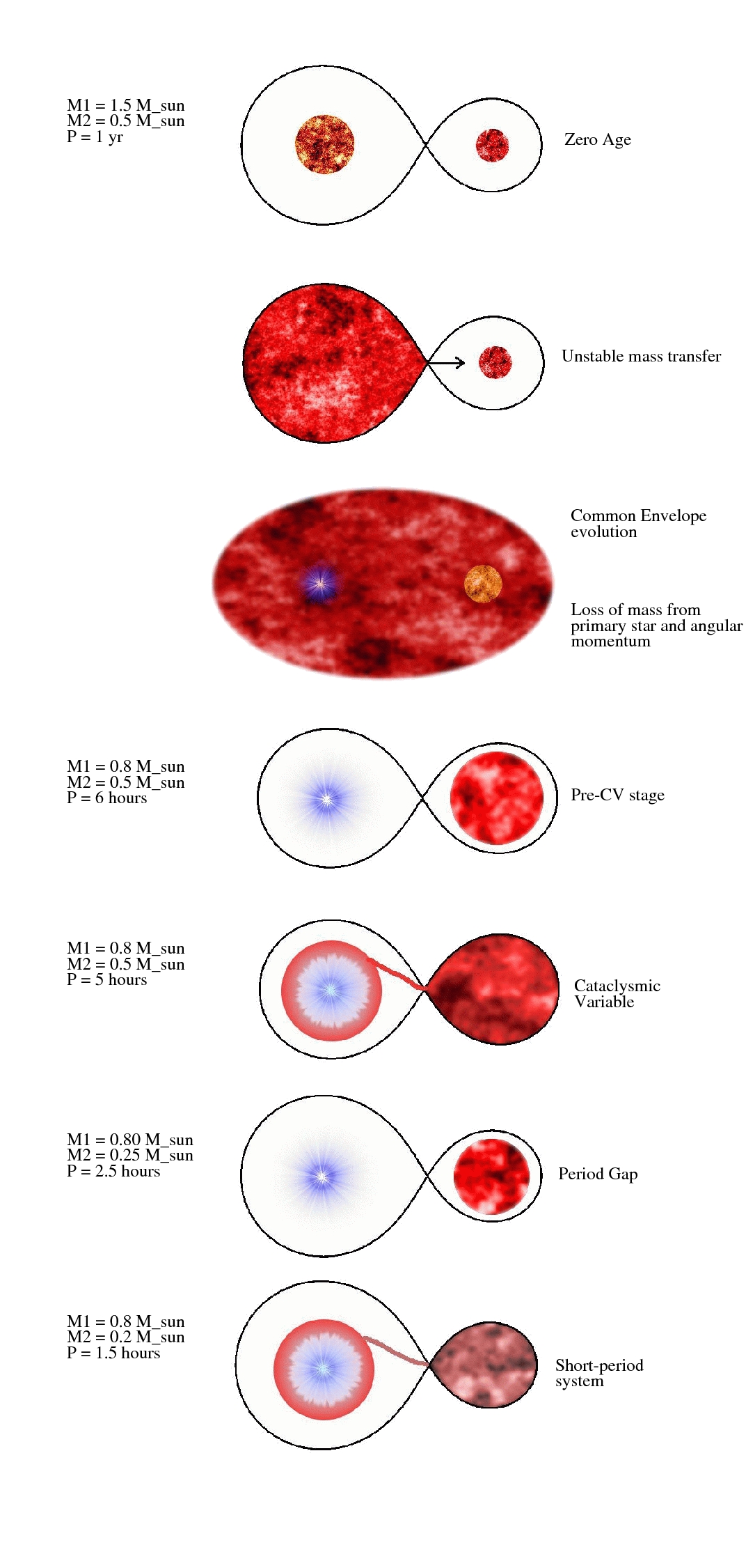
Figure 1.8: A schematic demonstrating the important stages in the evolution of a CV. The primary star is on the left and the secondary on the right. From Littlefair (2001).

1.4.6 The orbital period distribution

As one of the most easily, and most accurately, determined physical parameters, the distribution of the orbital periods of CVs potentially provides a useful window into their evolution. The orbital period distribution of CVs, shown in figure 1.9, has three main features: the minimum period, the long-period cut-off and the period gap.

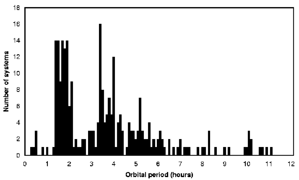
Figure 1.9: The orbital period distribution of CVs for periods less than 12 hours, compiled from Ritter & Kolb (1998).

The minimum period

There is an observed minimum period for CVs of approximately 78 minutes. This is due to the secondary star becoming degenerate for masses below $\sim 0.08\;{\rm M}_{\odot}$. The degenerate secondary effectively becomes a very low mass white dwarf, and as such (if in thermal equilibrium) will obey the mass-radius relationship for a white dwarf, for instance the analytical approximation to the Hamada-Salpeter relation (Hamada & Salpeter, 1961) of Nauenberg (1972):

$$R=7.795\times 10^{6}\left[\left(\frac{1.44\;{\rm M}_{\odot}}{M}\right)^{\frac{2}{3}}-\left(\frac{M}{1.44\;{\rm M}_{\odot}}\right)^{\frac{2}{3}}\right]^{\frac{1}{2}}\rm{m}.$$ (1.15)

Equation 1.15 illustrates that decreasing the mass of a degenerate secondary leads to expansion of its radius. For $q<2/3$ (see equation 1.14 and the following discussion), this situation is, surprisingly enough, stable (Warner, 1995, pages 459 & 462).

Once again, it is easiest to think of this continuous process as occurring in two stages: as $q<5/6$, mass transfer leads to the orbital separation and the size of the secondary’s Roche-lobe increasing (equations 1.7 and 1.9). The continuing mechanisms of orbital angular momentum loss then decrease the orbital separation and the secondary’s Roche-lobe until mass transfer can re-commence, but the secondary has in the meantime expanded in response to its mass loss, so mass transfer begins again at a slightly larger separation than before.

The long-period cut-off

Above an orbital period of about six hours the number of CVs declines, with very few observed with periods $>12$ hours. As seen in § 1.4.5, stable mass transfer requires that $q<1.26$. Since the mass-accreting star is a white dwarf, it has a maximum mass of $1.44\;{\rm M}_{\odot}$ (the Chandrasekhar mass). Kepler’s third law (equation 1.1) requires that the orbital separation increases as the orbital period increases. This results (equation 1.4) in the size of the Roche-lobe, and therefore the mass of the (dwarf) star required to fill it, increasing. The constraint on the maximum mass of the white dwarf thus leads to an upper limit on the orbital period of $\sim 12$ hours. The few systems with $P_{\rm{orb}}\geq 12$ hours have evolved secondaries. The fact that few white dwarfs actually have the Chandrasekhar mass naturally explains the gradual decline in the number of systems with $P_{\rm{orb}}\gtrsim 6$ hours.

The period gap

Between $2.2\leq P_{\rm{orb}}\leq 2.8$ hours there is a significant deficiency of systems. (Polars do not show this gap, but intermediate polars do.) A number of possibilities present themselves as explanations for this period gap. As shown in § 1.4, CVs evolve to shorter orbital periods due to angular momentum loss. This could imply that the CVs above and below the period gap are actually two separate populations. The upper bound of the period gap would then represent some minimum period for the long-period population, and the lower bound a maximum period for the short-period CVs. To produce a minimum orbital period of about three hours the secondary stars would have to be degenerate and of very low luminosity (Verbunt, 1984). This is not supported observationally, however: such stars are observed to have normal main-sequence luminosities (Warner, 1995, page 465).

The favoured scenario is that CVs evolve into the period gap from a single population, but cease mass transfer whilst they are in it. This obviously requires some sort of mechanism to halt mass transfer at the upper bound of the period gap: the disrupted magnetic braking model, the subject of the following section.

1.4.7 The disrupted magnetic braking model

The period gap is thought to be a consequence of a change in the internal structure of the secondary star. As noted by Robinson et al. (1981), at an orbital period of around three hours, which corresponds to a secondary mass of $\sim 0.25\;{\rm M}_{\odot}$ (Smith & Dhillon, 1998), the internal structure of the secondary changes from a radiative core ($M_{2}>0.3\;{\rm M}_{\odot}$) to a convective core ($M_{2}<0.3\;{\rm M}_{\odot}$). It is suspected that this interferes with the dynamo-generated magnetic field of the secondary (King, 1988), disrupting magnetic braking. Whatever the mechanism of the reduction of magnetic braking, if it results in $\tau_{\rm{KH}}<\tau_{\rm{MT}}$, where $\tau_{\rm{MT}}$ is the time-scale for mass transfer, it gives the secondary time to readjust its structure so that it can shrink back within its Roche-lobe, causing mass transfer to cease and establishing the upper edge of the period gap. (Remember that when mass transfer is occurring the secondary is larger than its equilibrium main-sequence radius; it is filling its Roche-lobe.)

Note that this explanation is rather speculative, since it assumes that magnetic braking is the dominant cause of angular momentum loss in systems above the period gap. Andronov et al. (2003, see also § 1.4.1) point out that it is not clear that this is true and that there is no observational evidence for a sudden cessation in magnetic braking at the point where the secondary switches from a radiative to a convective core.

1.5 The gas stream and accretion disc

The presence of accretion discs in many CVs accounts for much of the interest in these systems. Accretion discs are an incredibly widespread astrophysical phenomenon, occurring in a variety of locations and scales. They are present around young stars (T Tauri stars) where they assist the formation of the protostar by removing angular momentum from material in the collapsing gas cloud. They are also thought to be involved in the formation of planetary systems. At the other extreme, accretion discs fuel the cores of active galaxies, radiating the gravitational potential energy lost by material as it falls towards a central massive black hole. Unfortunately, however, accretion discs around young stars are shrouded by the dust and gas from which these stars are forming, and those in the cores of active galaxies are not only frequently obscured by the surrounding dust, gas and stars, but are at great distances. Additionally, the accretion discs present in CVs evolve more quickly than those in either T Tauri stars or the cores of active galaxies. One final advantage that observations of the discs in CVs have over those of T Tauri discs is that CV discs are hotter, and therefore more luminous at optical wavelengths. It is in CVs, therefore, specifically in eclipsing systems, that accretion discs are most profitably observed.

1.5.1 Gas stream dynamics

From the inner Lagrangian point to the point where it impacts the disc, the gas stream follows a ballistic trajectory, shown in figure 1.10. The equations of motion for a point mass in a Cartesian co-ordinate system co-rotating with the binary as described in § 1.2 are (e.g. Flannery, 1975; Dhillon, 1990):

$$\ddot{x}=\frac{GM_{1}}{r_{1}^{2}}\frac{(x_{1}-x)}{r_{1}}+\frac{GM_{2}}{r_{2}^{2}}\frac{(x_{2}-x)}{r_{2}}+2\omega\dot{y}+\omega^{2}r_{\rm{cm}}\frac{(x-x_{\rm{cm}})}{r_{\rm{cm}}}$$ (1.16)

and

$$\ddot{y}=\frac{GM_{1}}{r_{1}^{2}}\frac{(y_{1}-y)}{r_{1}}+\frac{GM_{2}}{r_{2}^{2}}\frac{(y_{2}-y)}{r_{2}}+2\omega\dot{x}+\omega^{2}r_{\rm{cm}}\frac{(y-y_{\rm{cm}})}{r_{\rm{cm}}},$$ (1.17)

where the subscript ‘cm’ denotes the distance to the centre of mass of the system and $\omega=2\pi/P_{\rm{orb}}$ is the angular frequency. The first two terms in equations 1.16 and 1.17 are from the gravitational influence of the primary and secondary stars, respectively; the third is from the Coriolis force and the fourth from the fictitious centrifugal force.

The position of such a test particle at a given time is an example of the well-known three-body problem. As there is no (known) explicit solution, the problem must be solved by numerical integration. The position, velocity and acceleration of a test particle are calculated at time intervals $\Delta t$. As this interval becomes smaller, the calculation becomes more accurate, but more CPU-intensive. High accuracy is necessary near the primary star, where the potential gradient is steep (see figure 1.3), but wasteful where the potential is relatively flat. A good compromise can be achieved by adjusting the time interval according to the relation

$$\Delta t=\Delta t_{\rm{in}}\left(\frac{R}{R_{{\rm L}1}}\right)^{2},$$ (1.18)

where $\Delta t_{\rm{in}}$ is the initial time interval and $R$ and $R_{\rm L1}$ are the distances of the test particle and ${\rm L}_{1}$ point from the primary star, respectively. This decreases the time interval as a function of the square of the distance from the primary star, which is appropriate since the force exerted on the particle by the gravitational attraction of the primary also varies with the square of the distance from the star.

An additional constraint is that the energy of the particle is conserved along its path, so that the quantity

$$E_{J}=\dot{x}^{2}+\dot{y}^{2}-2\Omega(x,y),$$ (1.19)

where

$$\Omega(x,y)=\frac{1}{2}\left[\frac{M_{2}R^{2}_{2}}{M_{1}+M_{2}}+\frac{M_{1}R^{2}_{1}}{M_{1}+M_{2}}\right]+\frac{M_{2}}{(M_{1}+M_{2})R_{2}}+\frac{M_{1}}{(M_{1}+M_{2})R_{1}},$$ (1.20)

called the Jacobi energy, remains constant (Warner & Peters, 1972). In practice, the Jacobi energy is subject to the constraint

$$\frac{\Delta E_{J}}{E_{J}}<{\rm tol},$$ (1.21)

where tol is the fractional accuracy required (typically $10^{-4}$).

From the constraint on the Jacobi energy, it follows that the stream cannot re-cross the critical potential, and always approaches it with a low velocity. If the Jacobi energy is not conserved for a given time-step calculation, then the time interval $\Delta t$ is reduced by a factor of two and the step re-calculated until equation 1.19 is satisfied.

The accuracy of the calculation can be further improved by use of a second-order Runge-Kutta technique. This involves calculating the acceleration of the particle at the start and end of the time interval, and then applying the mean of these to the particle over the time-step.

Due to its angular momentum, the gas stream will pass by the white dwarf and eventually loop back around and collide with itself. This impact will give rise to turbulent shocks which dissipate much of the kinetic energy of the stream. Angular momentum, however, is not so easily lost and the material will therefore settle into the lowest energy orbit for a given angular momentum: a circular one.

The minimum outer radius of the accretion disc can be derived by calculating the radius around the white dwarf at which orbiting material has the same angular momentum as material at the inner Lagrangian point. This circularisation radius $R_{\rm{min}}$ is given by (Verbunt & Rappaport, 1988, their equation 13):

$$R_{\rm{min}}\approx 0.0883+0.04858\log q^{-1}+0.11489\log^{2}q^{-1}$$

$$-0.020475\log^{3}q^{-1}\,. 10^{-3}<q<1$$ (1.22)

The maximum possible radius of the disc can be determined from consideration of simple periodic particle orbits. Particle trajectories for radii approaching the radius of the primary’s Roche lobe become significantly non-circular due to the gravitational influence of the secondary star. Assuming that the largest orbit that does not intersect with any others is the maximum radius of the accretion disc (this is sensible because larger orbits that intersect will dissipate energy and prevent growth of the disc) gives the so-called tidal radius, $R_{\rm{tidal}}$, an approximate relation for which is (Paczyński, 1977; Warner, 1995, page 57)

$$\frac{R_{\rm{tidal}}}{a}=\frac{0.6}{1+q}\,. 0.03<q<1$$ (1.23)

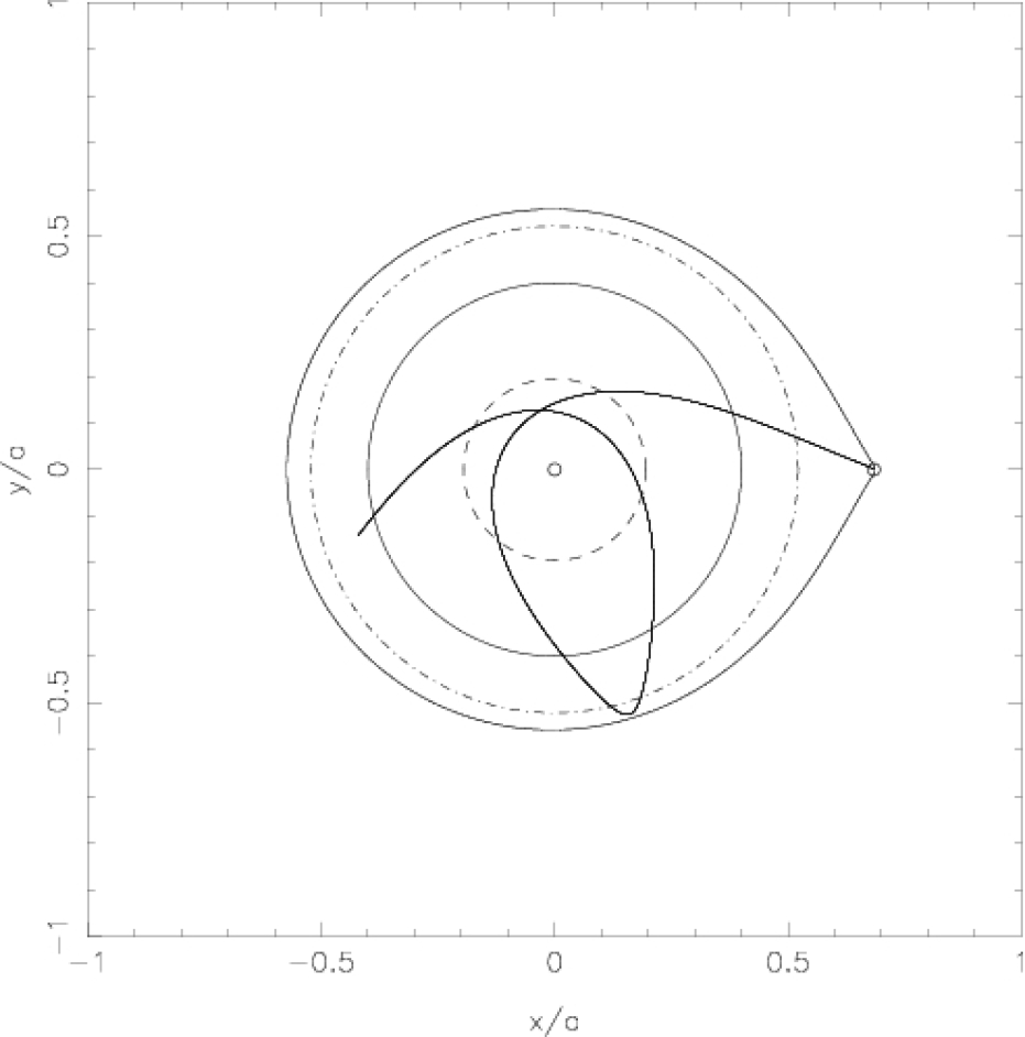
Figure 1.10: The trajectory of the gas stream for $q=0.15$. The stream originates at the inner Lagrangian point with a small initial velocity with respect to the binary frame. The minimum circularisation radius (Verbunt & Rappaport, 1988, their equation 13) is shown as the dashed circle, a disc radius of $0.4a$ is shown as a solid line, the dot-dash line is the tidal radius (Paczyński, 1977) and the Roche-lobe of the primary is the tear-drop shaped solid line. The position of the white dwarf at the origin is marked with an open circle, as is the inner Lagrangian point. The secondary star is to the right of the frame. Note that the stream does not re-cross the Roche-lobe.

1.5.2 The radial temperature profile

The velocities of the material in the accretion disc can usually be assumed to be negligibly different from Keplerian velocities, as at these distances from the primary the gravitational influence of the secondary star is slight. Viscosity in the disc occurs due to interaction between particles in slightly different orbits. Particles in smaller orbits orbit faster than material further out, and via viscous interaction speed up this outer material, transferring angular momentum to it, and vice versa. Angular momentum is therefore transferred outwards in the disc, resulting in a net flow of material inwards (Lynden-Bell & Pringle, 1974), driving accretion onto the white dwarf.

If we assume that all the potential energy $E_{p}$ lost by some mass $m$ as it spirals towards a mass $M$ from an initial radius $R$ to a radius $R-dR$ is radiated away as blackbody radiation, then the rate of energy release is

$$\Delta E_{p}=-GM\dot{m}\left(\frac{1}{R}-\frac{1}{R-dR}\right).$$ (1.24)

If we assume that the annulus defined by the radii $R$ and $R-dR$ emits as a blackbody, then we have

$$\Delta E_{p}=4\pi R\,dR\,\sigma T^{4}.$$ (1.25)

Combining equations 1.24 and 1.25 and setting $R-dR\approx R$ gives

$$T^{4}=\frac{GM\dot{m}}{4\pi R^{3}\sigma},$$ (1.26)

i.e.

$$T\propto R^{-3/4}.$$ (1.27)

This derivation neglects two effects. First, as material spirals to smaller radii its Keplerian velocity increases, so some of the gravitational energy released goes into the kinetic energy of the particles. Second, as material accretes onto the white dwarf, it decelerates to the rotation speed of the white dwarf in a boundary layer between the white dwarf and inner edge of the accretion disc. This deceleration results in kinetic energy being converted into thermal energy. With these factors taken into account, equation 1.26 becomes (Bath & Pringle, 1981; Horne & Cook, 1985)

$$T^{4}=\frac{3GM\dot{m}}{8\pi R^{3}\sigma}\left(\sqrt{1-R_{1}/R}\right),$$ (1.28)

where $R_{1}$ is the radius of the white dwarf.

In dwarf novæ in outburst and long-period novalikes, this simple $R^{-3/4}$ radial temperature profile is indeed observed by eclipse mapping experiments (Horne & Cook, 1985; Horne & Stiening, 1985; Rutten et al., 1992). In quiescent dwarf novæ a much flatter profile is observed (e.g. Wood et al., 1989a). This is thought to be because the disc does not achieve a steady state in quiescence (in a steady state the disc surface density does not evolve with time; $\partial\Sigma/\partial t=0$; see the following section).

1.5.3 Outbursts and the disc instability model

Dwarf nova outbursts have been observed and studied for well over a century. Outbursts of U Gem were first discovered in 1855 (Hind, 1856). Unsurprisingly, early attempts to explain dwarf nova outbursts tried to associate them with novæ and recurrent novæ. For several years the idea that dwarf novæ were just that, miniature novæ eruptions, was popular. In this scenario the outbursts are caused by a thermonuclear runaway of the hydrogen in the white dwarf envelope. Warner (1995, page 167 on) gives an excellent summary of early models of dwarf novæ outbursts.

The disc instability model was proposed by Osaki (1974). It attributes dwarf novæ outbursts to “sudden gravitational energy release due to intermittent accretion of material onto the white dwarf component … from the surrounding disc.” This intermittent accretion is triggered by an instability in the accretion disc. Osaki suggested that the secondary star transfers material at a constant rate, which is greater than the mass transfer rate through the disc. This would result in material accumulating in the accretion disc until some critical density were reached, whereupon the viscosity in the disc would increase greatly, enhancing the accretion rate onto the white dwarf (see § 1.5.2). The viscous heating of the disc results in an increase in the luminosity of the system. This follows from equation 1.28 and the Stefan-Boltzmann equation:

$$L=4\pi R^{2}\sigma T^{4},$$ (1.29)

which gives the bolometric luminosity of a blackbody of radius $R$ and temperature $T$, where $\sigma=5.67\times 10^{-8}$ Wm^-2K^-4 is the Stefan-Boltzmann constant.

Another consequence of the increase in the rate of angular momentum transportation is the expansion of the accretion disc, due to the conservation of angular momentum. Eclipse mapping of dwarf novæ during outburst has demonstrated this increase in the size of the accretion disc (figure 1.11).

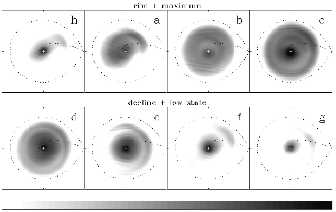
Figure 1.11: A sequence of eclipse maps of the dwarf nova EX Dra showing the rise (a–b) from quiescence (h) to maximum light (c), through the decline (d–f) to a low brightness state (g) that the system enters before recovering its quiescent brightness. The Roche-lobe and gas stream are shown as dotted lines, and the white dwarf at the centre is marked with a cross. The scale is logarithmic, with brighter regions indicated in black. From Baptista & Catalán (2001).

The viscosity of accretion discs

The exact mechanism of viscosity in accretion discs is non-obvious. Simple molecular viscosity is too weak to explain the rates of mass transfer through the disc necessary to reproduce the observed behaviour of accretion discs. Turbulence in the accretion disc could increase the viscosity, by causing globules of material to move to different orbits, transporting angular momentum between orbits at different radii.

Shakura & Sunyaev (1973) characterised the turbulence by the alpha viscosity $\alpha$. The alpha viscosity parameterizes the efficiency of the mechanism of angular momentum transport, and has a maximum of $\alpha=1$. The maximum size of the turbulent eddies is of the order of the disc thickness, $z_{0}$. The alpha viscosity prescription allows the viscosity $\nu$ to be quantified as

$$\nu=\alpha c_{\rm{s}}z_{0},$$ (1.30)

where $c_{\rm s}$ is the sound velocity.

This parameterization of the viscosity allows theoretical models of accretions discs, known as alpha discs, to be constructed by combining the alpha viscosity with the equations of gas dynamics. This leads to (Shakura & Sunyaev, 1973; Warner, 1995, page 47)

$$z_{0}\propto r^{9/8},$$ (1.31)

assuming that $\alpha$ is independent of radius. Equation 1.31 shows that alpha discs are concave, flaring out at their outer edges. Alpha discs are also ‘thin discs,’ i.e. their heights are small compared to their radii. Comparison of alpha disc models to observations shows that during outburst, values for $\alpha$ range from approximately 0.1 to 0.5, and during quiescence, from 0.01 to 0.05 (Mineshige & Wood, 1989; Warner, 1995, page 179; Hellier, 2001; Lasota, 2001; Schreiber, Hameury, & Lasota, 2003).

The disc instability model

The alpha viscosity itself gives no clue as to the cause of the turbulence. The key to this was developed in the 1990s, and is based on magnetic instabilities resulting in turbulence in the disc (Balbus & Hawley, 1991; Hawley & Balbus, 1991). Ionized material in the disc couples to the magnetic field in the disc, which forces material rotating more slowly (at larger radii) outwards and material rotating more quickly (at smaller radii) inwards. This stretches the field lines, amplifying them, and eventually leads to magnetic turbulence in the disc. The Balbus-Hawley or magneto-rotational instability has recently been demonstrated in the laboratory (Sisan et al., 2004).

The Balbus–Hawley instability provides a theoretical explanation of the trigger of dwarf novæ outbursts, in that it only operates when material in the disc is ionized. The disc of a dwarf nova in outburst is hot and highly viscous, whereas during quiescence it is cold and less viscous. All that is now required is some mechanism to cause heating of the disc in order to trigger the Balbus–Hawley instability and subsequently an outburst.

This mechanism is the thermal instability. The line of thermal equilibrium in the $\Sigma-T$ plane, where $\Sigma$ is the surface density of the material, is known as the ‘S-curve’ (shown in figure 1.12). On the S-curve, heating from viscous forces balances the radiation from the surface. A system located off this line of thermal equilibrium will heat or cool, as appropriate, until equilibrium is established on the S-curve. Not all equilibrium states are stable, however, only those that satisfy $dT/d\Sigma>0$. Those states with negative gradients ($dT/d\Sigma<0$) are unstable: a small positive perturbation of $\Sigma$ leads to an increase in $T$, which takes the state away from the S-curve of thermal equilibrium. To regain stability the system would have to migrate to lower $T$.

Consider first of all an unionized, cold annulus within an accretion disc. If the rate of mass transfer into the unionized annulus is greater than the rate at which material flows through it, it will inevitably begin to fill up, increasing the surface density. The greater surface density of the disc results in an increase in the viscosity, which in turn increases the temperature via viscous heating. The increase in viscosity also causes the mass transfer rate through the annulus to increase. As unionized hydrogen has a low opacity $\kappa$ to radiation, and this is not strongly dependent on temperature, the energy released by the viscosity will escape and the system will tend to stabilise itself on the lower branch of the S-curve. If, however, the annulus becomes hot enough ($\sim 7000$ K) for the hydrogen to become partially ionized, the situation changes. Unlike unionized hydrogen, the opacity of partially ionized hydrogen has a strong dependence on temperature: $\kappa\propto T^{10}$. The temperature rise therefore causes a massive increase in the opacity of the annulus, trapping the energy released by the viscosity, and further increasing the temperature. Although the viscosity increase means that the surface density of the region is being reduced, the effect this has on the temperature increase is vastly outweighed by the increase in the opacity-trapped energy.

Once the annulus is completely ionized, the opacity is no longer highly sensitive to temperature, and the annulus settles into equilibrium at a much higher temperature on the upper branch of the S-curve. The Balbus-Hawley instability can now kick in as the magnetic field is able to couple to the ionized material in the annulus, and the viscosity will increase. This means, however, that the rate of mass transfer through the annulus is greater than the rate of mass transfer into it, so the surface density of the annulus gradually decreases, and with it the temperature, until the hydrogen in the annulus becomes partially ionized again. The temperature-opacity dependence returns, and the opacity rapidly drops as the temperature falls, until the hydrogen becomes unionized and the viscosity returns to normal. This cycle is known as the thermal limit cycle, and is illustrated in figure 1.12; see Warner (1995, page 173 on) for a fuller discussion.

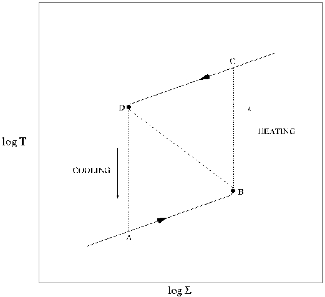
Figure 1.12: The $\Sigma-T$ relation and the resulting thermal limit cycle for dwarf novæ. At point A, the dwarf nova is at quiescence, with a cool, unionized disc. Material builds up in the disc, increasing the disc temperature, and the dwarf nova moves to point B. Here, the hydrogen in the disc becomes partially ionized, leading to a large opacity increase and subsequent runaway temperature increase to point C—the dwarf nova enters outburst. At point C, the hydrogen has become fully ionized, so the disc opacity becomes insensitive to temperature, halting the runaway temperature increase. Enhanced mass transfer through the disc onto the white dwarf due to the Balbus-Hawley instability leads to the surface density of the disc decreasing, and with it the temperature, until the hydrogen begins to recombine at point D. At this point the thermal instability begins to operate again, and the disc rapidly cools to point A. The S-curve comprises the solid and dashed lines. From Watson (2002).

The thermal instability described above begins in a certain annulus and then proceeds to the rest of the disc by distributing hot material to adjacent annuli. This heating wave can start either in the inner disc, in which case the resulting outburst is known as inside-out, or in the outer disc, leading to an outside-in outburst. Which type occurs depends on the mass transfer rate from the secondary star. At lower mass transfer rates, the material has time to filter through the disc, and accumulates at smaller radii. If the mass transfer rate from the secondary star is large, however, the material tends to build up nearer the outer edge of the disc. In the former case, an inside-out outburst results; in the latter, an outside-in. Inside-out outbursts tend to have a slower rise to outburst maximum than outside-in outbursts. This is due to three main factors:

1. Viscosity causes more material to flow inwards than outwards;

2. Inner radii have smaller surface densities ($\Sigma\propto R^{1.05}$, Cannizzo et al., 1988), so there is less material to spread outwards;

3. Outer radii are larger, so the surface density of material moving to larger radii is reduced, hampering the progress of the heating wave. Material travelling inwards has its surface density increased, thus aiding the progress of the heating wave.

1.5.4 Superoutbursts and superhumps: SU UMa stars

The definition of an SU UMa star (see § 1.3.2) is a dwarf nova that also exhibits superhumps. To date, no star has yet been found that exhibits superhumps but not superoutbursts, or vice versa, so I shall presume that the presence of one of these phenomena implies the other. The orbital period distribution of SU UMa stars is pronounced: they all (with the exception of TU Men) lie below the period gap. It is suspected that all dwarf novæ below the period gap are SU UMa stars (Warner, 1995, page 127).

The cause of superhumps is the precession of an elliptical disc (Vogt, 1982). The precession period $P_{\rm{prec}}$ of such a disc will create a beat, or superhump, period $P_{\rm{sh}}$ with the orbital period $P_{\rm{orb}}$:

$$\frac{1}{P_{\rm{sh}}}=\frac{1}{P_{\rm{orb}}}-\frac{1}{P_{\rm{prec}}}.$$ (1.32)

The origin of the elliptical disc is tidal resonances of particles in the outer disc with the secondary star (Whitehurst, 1988; Whitehurst & King, 1991). Particles with orbital periods in resonance with the orbital period of the secondary are forced, due to the gravitational interaction with the secondary, to follow non-circular orbits (see also § 1.5.1). The particles cannot, however, follow these orbits exactly, because they intersect both with neighbouring circular orbits and themselves. The non-circular orbit cannot be uniformly populated due to these self-interactions, so a precessing arc of material is formed. Interactions between this arc and the disc itself are thought to produce the superhump light (see figure 1.13).

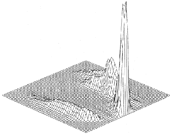
Figure 1.13: The superhump light distribution across the disc of the SU UMa star Z Cha during superoutburst. The primary is at the centre of the grid (which has sides equal to the orbital separation) and the secondary off the grid at bottom right. The superhump light originates from three regions at the rim of the disc where particle orbits intersect. The plot has been produced by maximum-entropy eclipse mapping, and is taken from O’Donoghue (1990).

1.5.5 Spiral shocks

Spiral shocks are another manifestation of the tidal influence of the secondary star on the accretion disc. They are density waves formed in the disc when particles in intersecting, non-circular orbits interact (Sawada et al., 1986a, b). The shock waves form a two-armed spiral pattern in the disc and are capable of transporting angular momentum through the disc without the need for viscosity (see § 1.5.3). Spiral shocks were first detected in the outburst accretion disc of the dwarf nova IP Peg (Steeghs et al., 1997, 1998) and have since been observed in many other CVs, including V347 Pup (Still et al., 1998), EX Dra (Joergens et al., 2000), U Gem (Groot, 2001) and WZ Sge (Baba et al., 2002). Until recently, spiral shocks had only been observed in either outburst or a high state, but there is some recent evidence for spiral shocks in the quiescent discs of IP Peg (Neustroev et al., 2002) and U Gem (Morales-Rueda, 2004; Unda-Sanzana, 2005).

1.6 Methods of mass determination

The mass ratio and the component masses are, apart perhaps from the orbital period, the most fundamental physical parameters of any binary star system. A knowledge of the component masses is central to our understanding the origin, evolution and behaviour of CVs. Population synthesis models (e.g. de Kool, 1992) and the disrupted magnetic braking model (§ 1.4.7) of CV evolution are just two crucial aspects that require reliable masses in order to be observationally tested. Unfortunately, at present reliable CV mass estimates are limited to approximately 20 systems, partially due to the intrinsic difficulties in obtaining such masses (see Smith & Dhillon (1998) for a review).

1.6.1 Mass-orbital period relations

Reasonable estimates of the masses of the secondary stars in CVs can be obtained from the mass-orbital period relationship (Robinson, 1973, 1976; Warner, 1995, page 106). Note that equation 1.1 can be rewritten as

$$\frac{M_{2}}{{\rm M}_{\odot}}=0.358\left(\frac{1+q}{q}\right)^{\frac{1}{2}}\left(\frac{R_{\rm{L}}}{a}\right)^{\frac{3}{2}}\left(\frac{M_{1}}{{\rm M}_{\odot}}\frac{{\rm R}_{\odot}}{R_{\rm{L}}}\right)^{\frac{3}{2}}P_{\rm{orb}}(\rm{h}).$$ (1.33)

The first two terms in brackets are virtually independent of the mass ratio $q$. The last can be determined from any mass-radius relationship. Following Warner (1995, page 106), I adopt the empirical result for low-mass ($<0.5\;{\rm M}_{\odot}$) main-sequence stars of Caillault & Patterson (1990), as appropriate for the secondary stars in CVs:

$$\frac{R}{{\rm R}_{\odot}}=0.918\left(\frac{M}{{\rm M}_{\odot}}\right)^{0.796}.$$ (1.34)

Combining these last two equations with equation 1.8 gives an approximate mass-period relationship for the secondary stars in CVs:

$$\frac{M_{2}}{{\rm M}_{\odot}}\approx 0.091P^{1.44}_{\rm{orb}}(\rm{h}).$$ (1.35)

Smith & Dhillon (1998) obtained an empirical mass-period relation for the secondary star from CVs with well-determined component masses:

$$\frac{M_{2}}{{\rm M}_{\odot}}=(0.126\pm 0.011)P_{\rm{orb}}({\rm h})-(0.11\pm 0.04).$$ (1.36)

Although such a method of mass determination is obviously not entirely satisfactory, mass-period relations such as equations 1.35 and 1.36 provide a means of estimating the secondary mass in a CV from what is often the only available observational constraint: the orbital period. Unfortunately, they provide no clue as to the mass of the primary star.

1.6.2 Radial velocity mass determination

The masses of the primary and secondary star can be directly determined if the radial velocities of the stellar components $K_{1}$ and $K_{2}$ and the orbital period and inclination are accurately known.

Observed at an inclination $i$, the radial velocity amplitude of the primary is

$$K_{1}=\frac{2\pi a_{1}}{P_{\rm{orb}}}\sin i$$ (1.37)

and that of the secondary is

$$K_{2}=\frac{2\pi a_{2}}{P_{\rm{orb}}}\sin i.$$ (1.38)

From

$$a=a_{1}\left(\frac{M_{1}+M_{2}}{M_{2}}\right)$$ (1.39)

and Kepler’s third law (equation 1.1), we then obtain the standard relationships for the mass functions $f$ of the primary

$$f(M_{1}) = \frac{P_{\rm{orb}}K^{3}_{2}}{2\pi G}$$ (1.40a)

$$= \frac{(M_{2}\sin i)^{3}}{(M_{1}+M_{2})^{2}}$$ (1.40b)

$$= M_{1}\left(\frac{q}{1+q}\right)^{2}\sin^{3}i$$ (1.40c)

and of the secondary

$$f(M_{2}) = \frac{P_{\rm{orb}}K^{3}_{1}}{2\pi G}$$ (1.41a)

$$= \frac{(M_{2}\sin i)^{3}}{(M_{1}+M_{2})^{2}}$$ (1.41b)

$$= M_{2}\left(\frac{1}{1+q}\right)^{2}\sin^{3}i.$$ (1.41c)

Note that the mass functions are functions of the observable quantities $K$ and $P_{\rm{orb}}$ only. As the mass ratio $q$ is given by

$$q=K_{1}/K_{2}=M_{2}/M_{1},$$ (1.42)

the orbital inclination is all that is needed to gain accurate individual masses if the mass functions are known. However, the inclination is generally only reliably determined in eclipsing systems. The fact that a system exhibits eclipses at all constrains the inclination to $60^{\circ}\lesssim i<90^{\circ}$ (figure 1.14). An eclipse of the white dwarf further limits the inclination to $75^{\circ}\lesssim i<90^{\circ}$. The presence of distinct eclipses of the white dwarf and bright spot allows, as discussed in the following section, accurate determination of both the mass ratio and orbital inclination.

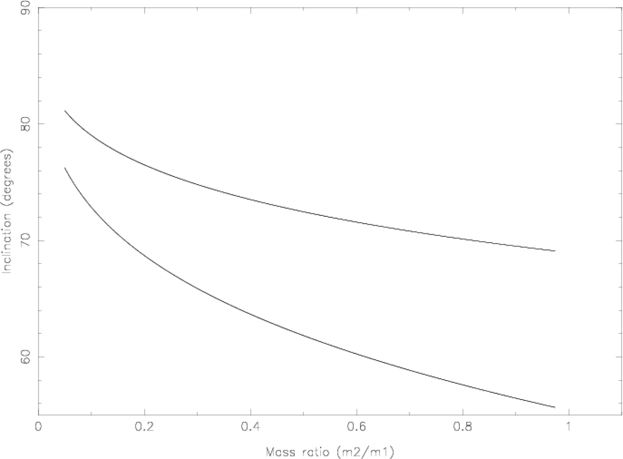
Figure 1.14: The relationship between the mass ratio $q$ and orbital inclination $i$ for grazing eclipses ($\Delta\phi=0$) of (bottom) the bright spot and (top) the white dwarf. The disc radius is $0.35a$.

The orbital inclination can also be estimated in non-eclipsing systems from modelling of ellipsoidal variations (Russell, 1945) from the secondary star (e.g. Sherrington et al., 1982; Berriman et al., 1983; McClintock et al., 1983), but this requires accurate modelling of reflection effects and gravity- and limb-darkening (e.g. Lucy, 1967; Pantazis & Niarchos, 1998; Claret & Hauschildt, 2003). Smith & Dhillon (1998) describe various other methods by which estimates of stellar masses in CVs may be made, but in general eclipsing systems are the only ones for which we know reliable inclinations (Warner, 1995, page 103).

Measuring the radial velocity amplitude of the white dwarf is problematic. The white dwarf (absorption) lines usually only dominate in the ultra-violet, and are hence generally unobservable from below-atmosphere sites. Sion et al. (1998) obtained a direct measurement of the white dwarf radial velocity amplitude of U Gem from Hubble Space Telescope (HST) observations using the Si iii absorption line. In general, however, $K_{1}$ has to be measured from optical emission lines of the accretion disc. For an azimuthally symmetric disc, these lines trace the orbital motion of the primary. Problems arise when the disc departs significantly from this symmetry, due primarily to interactions between the disc and gas stream in the region of the bright spot. This gives rise to phase shifts and apparent orbital eccentricities in the radial velocity curves. Techniques that determine the radial velocity amplitude from the emission line wings (e.g. the double-Gaussian method of Schneider & Young, 1980) presume that most of the asymmetric emission originates in the outer disc (Horne et al., 1986) where the disc-stream interaction should be maximised. Frequently, however, this does not solve the problem (e.g. Thoroughgood et al., 2004), and the emission lines are asymmetric at all radii. The radial velocity distortions can be either due to asymmetric brightness distributions (e.g. Stover, 1981), perhaps due to the gas stream overflowing the edge of the disc and impacting the disc at smaller radii (Lubow & Shu, 1975), and/or to non-Keplerian velocity distributions (e.g. Schoembs & Hartmann, 1983; Marsh et al., 1987). Equation 1.41a shows that the mass function is highly dependent on an accurate determination of $K_{1}$; for the most part making the use of uncertain values of $K_{1}$ in mass determinations unwise.

For the above reasons, radial velocity studies generally concentrate on $K_{2}$. Although absorption lines from the secondary can be observed at the red end of the spectrum, the continuum emission is often dominated by the disc. Cross-correlation of the CV spectrum with a template of a cool dwarf spectrum (Stover et al., 1980) is often used to obtain the radial velocity amplitude of the secondary. Summing phase-binned spectra followed by such cross-correlation can reveal many weak absorption lines from the secondary (Horne et al., 1986). A technique known as skew-mapping, which also makes use of cross-correlation of CV and template star spectra, is useful in cases where the signal-to-noise ratio is poor. Vande Putte et al. (2003) describe the method in detail; it entails finding the peak of the line integral of the cross-correlation function in the $(K_{1},K_{2})$ plane.

Rotational broadening of the secondary’s absorption lines can also be used to determine the value of $v\sin i$ for the secondary, where $v$ is the rotational velocity of the secondary. As the secondary star is tidally locked, its rotation period is identical to the orbital period, yielding (Friend et al., 1990; Horne, Welsh, & Wade, 1993)

$$\frac{R_{2}}{a}(1+q)=\frac{v\sin i}{K_{2}}.$$ (1.43)

Using equation 1.4 for the volume radius of the Roche-lobe together with the above expression allows the mass ratio to be determined (e.g Horne et al., 1993; Thoroughgood et al., 2001). The inclination can then be determined from the unique relation between the mass ratio and orbital inclination for a given eclipse width of the primary $\Delta\phi$ (Bailey, 1979; see figure 1.14), which can be understood as follows:

1. At smaller orbital inclinations a larger secondary radius $R_{2}$ is required in order to produce a given eclipse width.

2. The secondary radius is defined by the mass ratio because the secondary fills its Roche lobe.

3. Therefore for a specific white dwarf eclipse width $\Delta\phi$ the inclination is known as a function of the mass ratio.

Remember that the shape of the system does not depend on the orbital separation $a$: this just determines the scale.

The relation between the eclipse width, orbital inclination and secondary radius is often approximated by the eclipse of a point source by a spherical body, which gives the analytical expression (Dhillon et al., 1991)

$$\left(\frac{R_{2}}{a}\right)^{2}=\sin^{2}(\pi\Delta\phi)+\cos^{2}(\pi\Delta\phi)\cos^{2}i.$$ (1.44)

For an axi-symmetric disc the white dwarf eclipse phase width $\Delta\phi$ is approximately equal to the full phase width at half maximum of the disc eclipse $\Delta\phi_{1/2}$ (e.g. Dhillon, 1990). If the disc eclipse is symmetrical about phase zero then this is a good approximation. The radius of the secondary can then be determined from the mass ratio. Kepler’s third law (equation 1.1) then allows the rest of the system parameters, including the stellar masses, to be determined.

Such mass estimates from the radial velocity of the secondary, however, can run into problems if the secondary flux is not uniform across the surface of the star. Effects such as gravity- and limb-darkening need to be accounted for, but the major problem is irradiation from the primary. This results in absorption features being eliminated from (or reduced in strength on) the illuminated face of the secondary, a problem made more complex by the fact that regions of the secondary star will be shadowed by the accretion disc, so will still show absorption lines. This scenario results in an asymmetric line flux distribution across the secondary star, which can adversely affect the measurement of $K_{2}$. For example, if the absorption lines are reduced in strength on the side of the secondary facing the primary, then the flux from the absorption lines will be centred towards the far side of the secondary. The measured value of $K_{2}$ will therefore be larger than the true, dynamical, value. As an example of how this can be corrected for, Thoroughgood et al. (2004) used model CV spectra with varying numbers of vertical slices across the inner hemisphere of the secondary star’s Roche-lobe omitted in order to model the irradiation of the inner face of the star, leading to a corrected value of $K_{2}$.

1.6.3 The photometric method of mass determination

In a number of eclipsing objects, the component masses may be determined from photometry combined with a mass-radius relation for the primary (e.g. Wood et al., 1986). This results in a purely photometric model of the system, untroubled by concerns about the contamination of $K_{1}$ or $K_{2}$. This technique is thus both a valuable method of determining the masses in itself, and a useful check of spectroscopic results. Table 1.1 compares the results achieved by reliable spectroscopic techniques to those found via photometry alone. The agreement between the values quoted is good, however, many spectroscopic determinations of the mass ratio for other dwarf novæ have been excluded due to unreliable techniques being employed. The conclusion to be drawn is that both methods can produce reliable and accurate values, but that great care must be taken when using spectroscopic data (see Smith & Dhillon, 1998 for a detailed discussion of the techniques of mass determination).

Table 1.1: A comparison of purely spectroscopic and purely photometric determinations of the mass ratios of selected dwarf novæ. Only those dwarf novæ with mass ratios accurately determined by both spectroscopy alone and photometry alone are shown, as the use of inappropriate data and/or techniques can result in wildly inaccurate results. See Smith & Dhillon (1998) for a critical discussion of the (then) available mass estimates of CVs. The photometric determinations listed below all use the method described in § 1.6.3. The spectroscopic determinations used the following techniques. V2051 Oph: Ref. 1 used $K_{1}$ from H$\beta$ and H$\gamma$, corrected for disc asymmetry, the radial velocities of the disc emission lines and the eclipse width from the continuum light curve. IP Peg: Ref. 3 used $K_{2}$ from TiO absorption features combined with the projected rotational velocity of the secondary star as determined by Catalán (private communication); ref. 4 used Roche tomography. EX Dra: Ref. 6 used $K_{1}$ measured from H$\beta$, H$\gamma$ and H$\delta$ using the double-Gaussian method of Schneider & Young (1980) and $K_{2}$ measured from calcium absorption lines.

Object	Spectroscopic		Photometric
	$q$	Ref.	$q$	Ref.
V2051 Oph	$0.26\pm 0.04$	1	$0.19\pm 0.03$	2
IP Peg	$0.322^{+0.075}_{-0.037}$, $0.43$	3, 4	$0.35<q<0.49$	5
EX Dra	$0.75\pm 0.01$	6	$0.72\pm 0.06$	7

References:	1. Watts et al. (1986), 2. Baptista et al. (1998),
	3. Beekman et al. (2000), 4. Watson et al. (2003),
	5. Wood & Crawford (1986), 6. Fiedler et al. (1997),
	7. Baptista et al. (2000).

The most fundamental requirement of the photometric technique is the presence of clear and distinct eclipses of the white dwarf and bright spot. An example of such a system is OY Car, illustrated in figure 1.15. The method then proceeds by utilising the unique relationship between $q$ and $i$ for a given $\Delta\phi$ (see the previous section and figure 1.14).

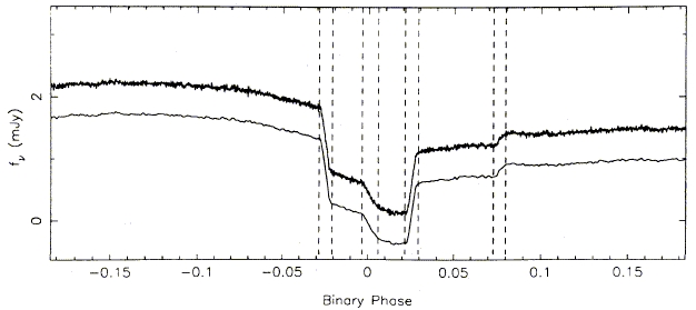
Figure 1.15: An eclipse of OY Car, illustrating the distinct eclipses of the white dwarf and bright spot. From left, marked by pairs of vertical dashed lines (i.e. the start and end): the ingress of the white dwarf; the ingress of the bright spot; the egress of the white dwarf and the egress of the bright spot. The upper curve is the raw data and the lower curve the data after smoothing. Adapted from Wood et al. (1989a).

If it is assumed that the ballistic gas stream, the trajectory of which can be determined as described in § 1.5.1, passes through the position of the bright spot, by calculating and comparing the ingress and egress phases of each point along the gas stream for different values of $q$ to those of the bright spot eclipse timings the mass ratio and orbital inclination can be uniquely determined. The additional assumption that the bright spot lies on the outer edge of the accretion disc gives the radius of the disc. To obtain the component masses, a mass-radius relation for the primary is required, for instance the Nauenberg approximation (equation 1.15). This method of determining the system parameters is discussed in more detail in § 3.2.

1.7 This thesis

Chapter 2 describes the observations and the reduction procedure employed on the data obtained. I give a detailed review of the ultracam instrument, give full details of the observations discussed in the latter portions of this thesis and elucidate the procedures used to reduce the data. In chapter 3, I describe the analysis techniques I applied to this data and a detailed comparison of two distinct methods of photometric parameter determination. I also describe the eclipse mapping method. The structuring of the three results chapters mirrors that of the three papers that this thesis is based upon, and is roughly chronological. The results for the system parameters for OU Vir are given in chapter 4 and those for XZ Eri and DV UMa in chapter 5. Observations of GY Cnc and IR Com are described and discussed in chapter 6. The main subject of this latter chapter is, however, a discussion of the results of eclipse mapping of the quiescent disc of HT Cas in two distinct states in 2002 and 2003. The results of eclipse mapping experiments for the other objects are given at the end of the relevant chapter. I conclude in chapter 7 with a discussion of the main results of this thesis, and suggest some appropriate future work.

Chapter 2 Observations and data reduction

All the data presented in this thesis come from observations made with ultracam on the 4.2-m William Herschel Telescope (WHT) at the Isaac Newton Group of Telescopes, La Palma. The ultracam instrument is described in detail below; see also Dhillon & Marsh (2001), Beard et al. (2002), Dhillon et al. (2005), Stevenson (2005).

2.1 Ultracam

Ultracam is an ultra-fast, triple-beam CCD camera. A ray-trace of ultracam is shown in figure 2.1. A CAD image of the opto-mechanical design of ultracam is shown in figure 2.2 and a photograph of the instrument itself is shown in figure 2.3. Light from the telescope first passes through a collimator (which is interchangeable, allowing ultracam to be mounted on a variety of telescopes). It then encounters the first of two dichroic beam-splitters, which reflects light short-wards of $\sim 390$ nm through $90^{\circ}$, allowing longer wavelengths through. The longer-wavelength light then strikes the second dichroic. The cut-point for this beam-splitter is $\sim 550$ nm, and light of a wavelength shorter than this is reflected through $90^{\circ}$ (in the opposite direction to the blue light), while the rest is transmitted. The light is now split into three wavelength-dependent components. Each passes through re-imaging optics and the relevant filter (discussed below) before falling onto one of the three CCD detectors.

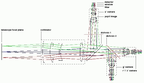
Figure 2.1: A ray-trace through ultracam, showing the major optical components: the collimator, dichroics, cameras, filters and detector windows. From Dhillon et al. (2005).

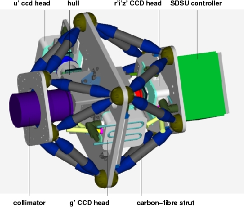
Figure 2.2: A CAD image of the opto-mechanical design of ultracam, highlighting some of the components discussed in the text and shown in the ray-trace of figure 2.1. From Dhillon et al. (2005).

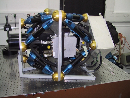
Figure 2.3: A photograph of ultracam in the test focal station of the WHT just prior to commissioning on the telescope (courtesy of Sue Worswick).

Ultracam uses the u^′g^′r^′i^′z^′ filter system defined by the Sloan Digital Sky Survey (SDSS; see Fukugita et al., 1996; Smith et al., 2002). The filter transmission functions are shown in figure 2.4. The importance of this choice of filter system is three-fold:

1. The u^′g^′r^′i^′z^′ filter system is likely to become the dominant filter system in the future, as the SDSS will survey the sky in unprecedented depth and detail.

2. Overlaps between the filters are minimised compared to the UBVRI system. This is of vital importance considering the dichroic beam-splitters used in ultracam.

3. The SDSS r^′ filter has a curtailed red wing compared to the Cousins R filter. This eliminates fringing with thinned chips in the r^′ filter.

The SDSS filter system is also useful in that it is a very broad band system—the bandpasses are significantly wider than other filter systems (Fukugita et al., 1996). This ensures high efficiency, which is useful when observing faint targets.

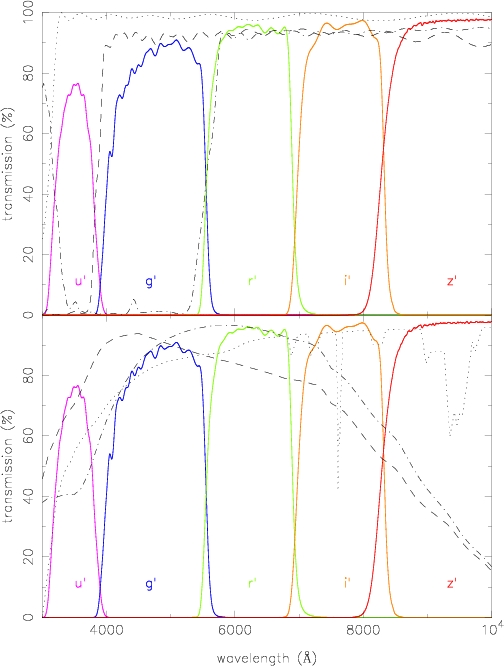
Figure 2.4: Top: Transmission profiles of the ultracam SDSS filter-set (solid lines), the anti-reflection coating used on the ultracam lenses (dotted line), and the two dichroics (dashed line and dashed-dotted line). Bottom: Transmission profiles of the ultracam SDSS filter-set (solid lines) and the atmosphere for unit airmass (dotted line). Also shown are the quantum efficiency curves of the u^′ and g^′ CCDs (dashed line) and the r^′i^′z^′ CCD (dashed-dotted line). From Dhillon et al. (2005).

The ability of ultracam to observe simultaneously in three colours is a crucial aspect of its design. Three colours enables a stellar spectrum to be distinguished from a blackbody. Simultaneous observations also eliminate the problem of the source varying between filter changes, crucial for observations of rapidly varying targets such as close binary stars.

The CCDs used in ultracam are key to its high time-resolution. The chips used are three Peltier-cooled (see § 2.3.3 for a discussion of why this is necessary), back-illuminated, anti-reflection coated (see figure 2.4), thinned EEV 47-20 frame-transfer CCDs with an imaging area of $1024\times 1024$ pixels ($13.3\times 13.3$ mm), giving a plate scale of $0.3^{\prime\prime}/{\rm pixel}$ on the WHT. This gives a field-of-view of $5^{\prime}$ on the WHT. At a Galactic latitude of $30^{\circ}$ (the all-sky average), this means that the probability of finding a comparison star brighter than 13 magnitudes is 0.96 (calculated using the on-line ultracam comparison star probability calculator, written by Vik Dhillon).

Frame-transfer CCDs have a masked-off storage area. Charge from the exposed portion of the chip is shifted (or vertically clocked) into this region before being horizontally clocked and digitized. This has the advantage that horizontal clocking and digitization can occur whilst the next exposure is taking place. This can vastly reduce the dead-time between exposures, since the digitization time is typically much greater than the clocking times (the digitization time is $\sim 6$ sec for the full-frame for ultracam). The vertical clocking speed for the chips used in ultracam is $24\;\mu{\rm s}\,/\,$row, which comes to $\sim 24$ ms for the total 1024 rows of pixels of the ultracam CCDs. As long as the exposure time is longer than the sum of the horizontal clocking and digitization times, the dead-time is reduced to the vertical clocking time.

Another useful, indeed crucial, aspect of the design of ultracam is the ability to only read out selected parts of the CCDs, called windows. This reduces the digitization time, and therefore the readout time, enabling higher frame rates to be achieved.

Ultracam also has a mode known as drift mode. In this mode a pair of windows are vertically clocked until they are just within the masked-off region of the chip, whereupon another pair of windows are exposed. In this way a vertical stack of windows is produced, and the dead time between exposures is much reduced. The stack of windows are continually shifted down the exposed and masked areas of the chip before being read out at the bottom. New windows are continually added at the top of the exposed area of the chip. Drift mode allows frame rates of up to 500 Hz to be realised. Stevenson (2005) discusses this in detail.

2.2 Journal of observations

Table 2.1 presents a full journal of observations. All the objects are dwarf novæ observed in quiescence, although OU Vir shows some evidence (see chapter 4) for being on the descent from superoutburst in both 2002 May and 2003 May. In the case of the 2003 May observations, this is supported by the detection of a superoutburst on May 2 by Kato (2003).

The observers in 2002 May (the commissioning run) were Vik Dhillon, Tom Marsh, Mark Stevenson, Paul Kerry, Carolyn Brinkworth, David Atkinson and Andy Vick. In 2003 May, the observers were Vik Dhillon, Tom Marsh, myself, Carolyn Brinkworth and Paul Kerry. In 2003 November, the observers were Tom Marsh and myself.

Table 2.1: Journal of observations. All dates are the start of the nights’ observing. The r^′ extinction is taken from the ING website, www.ing.iac.es, and is measured nightly by the Carlsberg Meridian Telescope. Values marked by a colon (:) are uncertain, probably due to the night being non-photometric.

Target	Date	Filters	UT start	UT end	Exposure	Seeing	Data	Cycle	Eclipses	$r^{\prime}$ extinction
	(yyyy mm dd)		(hh:mm)	(hh:mm)	time (sec)	(arcsec)	points			(mag/airmass)
OU Vir	2002 05 16	u′g′r′	23:38	02:18	0.5	1.2	1685	9442–9443	2	0.124
	2002 05 18	u′g′r′	00:20	00:25	1.7	2.1	59	1538	0	0.107
	2002 05 18	u′g′r′	00:26	02:10	4.0	2.1	1538	9470	1	0.107
	2003 05 19	u′g′z′	01:30	02:35	9.2	4.5	430	14504	0	0.188:
	2003 05 20	u′g′i′	01:14	02:36	5.2	1.2	933	14518	1	0.092:
	2003 05 22	u′g′i′	22:58	23:25	4.2	0.8	373	14544	1	0.234
	2003 05 25	u′g′i′	00:05	00:41	4.2	1.5	548	14586	1	0.115
DV UMa	2003 05 20	u′g′i′	23:06	23:40	5.9	1.3–2.0	339	69023	1	0.092:
	2003 05 22	u′g′i′	22:26	22:54	4.9	1.2	345	69046	1	0.234
	2003 05 23	u′g′i′	23:03	23:08	3.9	1.0	60	69058	0	0.383
	2003 05 23	u′g′i′	23:08	23:44	3.9	1.0	540	69058	1	0.383
XZ Eri	2003 11 13	u′g′i′	23:25	01:48	7.0	1.0–2.0	1225	4733–4734	2	0.073
GY Cnc	2003 05 19	u′g′z′	21:00	22:20	2.1	$\gtrsim 3$	2256	6826	1	0.188:
	2003 05 23	u′g′i′	22:02	23:01	1.6	1	2150	6849	1	0.383

Table 2.1: Continued. Journal of observations. The i^′ sensitivity was lost during the 2002 September 14 eclipse of HT Cas due to a technical problem with this band. The GPS signal, used for time-stamping each exposure, was lost for the HT Cas data of 2003 October 29. This means that the absolute time of each exposure was incorrectly recorded, although the relative timing within the run remains accurate. The cycle number for the data of 2003 October 29 is therefore estimated from times in the observing log. Due to poor weather, the extinction could not be measured for this night, and is therefore assumed to be 0.1 mag/airmass in the r^′ band, the mean of the previous and subsequent nights’.

Target	Date	Filters	UT start	UT end	Exposure	Seeing	Data	Cycle	Eclipses	$r^{\prime}$ extinction
	(yyyy mm dd)		(hh:mm)	(hh:mm)	time (sec)	(arcsec)	points			(mag/airmass)
IR Com	2003 05 21	u′g′i′	23:49	00:26	3.2	1	676	37857	1	0.197
	2003 05 23	u′g′i′	23:50	00:29	3.2	1	720	37880	1	0.383
	2003 05 25	u′g′i′	21:39	22:28	3.2	1.5	901	37902	1	0.115
HT Cas	2002 09 13	u′g′i′	23:13	01:00	1.1	1.2	5651	119537	1	0.089
	2002 09 14	u′g′i′	22:43	00:23	0.97–1.1	1.3–2.3	5470	119550	1	0.071
	2003 10 29	u′g′i′	–	–	1.3	1.4	4659	125116	1	0.1:
	2003 10 30	u′g′i′	19:25	22:01	1.3	1.0–1.5	6930	125129–125130	2	0.084

2.3 Data reduction

In this section I describe the data reduction procedure. Excepting GY Cnc, all the data were reduced by myself using the optimal extraction algorithm (Naylor, 1998) incorporated in Tom Marsh’s ultracam pipeline data reduction software, which resulted in a significant improvement in the signal-to-noise ratio over ‘normal’ extraction at low count rates (the u^′ data in particular; see § 2.3.4). The data for GY Cnc were reduced using the pipeline data reduction software with normal aperture photometry, due to a problem with the optimal extraction at high count rates.

Subsequent analysis was conducted by myself. Transparency variations were removed by dividing the target counts by that of a comparison star. Times were converted from modified Julian dates on the UTC time-scale (MJD) to heliocentric Julian dates (HJD) using the fruit Fortran subroutine, written by Peter Young. The comparison star counts were converted to SDSS magnitudes using observations of standard stars (Smith et al., 2002). All the data were corrected to zero airmass using the procedure discussed in detail in § 2.3.5.

2.3.1 Bias frames

The presence of readout noise, which occurs when digitizing charge in each pixel of the CCD, necessitates the addition of a (near) constant number of counts to each pixel: the bias. If this bias were not added, a systematic error would result when reading out low counts, since negative counts are not recorded by the analogue-to-digital converter. A bias frame can be obtained by taking a zero second exposure. In practice, with ultracam, an exposure time of 1 ms (the minimum exposure time permitted by the camera control software), in dark conditions, was used to take bias frames.

The high time-resolution of ultracam means that many bias frames were taken. These were combined using a clipped mean (at the $3\sigma$ level) to create a high signal-to-noise master bias frame free of cosmic rays. The master bias was subtracted from each data frame automatically by the pipeline software.

2.3.2 Flat fielding

The sensitivity of the CCD may vary across its surface. This variation occurs on both small scales (pixel-to-pixel variations in area) and large scales (e.g. vignetting, dust on the chip). These problems can be corrected by using a flat field.

A flat is created by taking an exposure of a uniform field of light. The best such field is usually an empty area of the twilight sky. Due to the inevitable presence of some (faint) field stars, the telescope was stepped in a spiral pattern during the flat field exposures. The resulting flats were then combined into a master flat field for use by the pipeline software by the following procedure.

First, the master bias was subtracted from each individual flat frame. The individual frames were then combined into a master flat using the ‘makeflat’ procedure in the pipeline software. This ignores all frames with counts above or below a certain level ($30\,000$ and $7\,000$, respectively). High counts may mean that the exposure is saturated, distorting the shape of the flat. Also, above counts of $\sim 30\,000$ a ‘peppering’ effect occurs on the ultracam CCDs. This effect is when adjacent pixels have high and low count levels, resulting in a chequered appearance across the chip. The cause of this effect is currently unknown (Stevenson, 2005). At the other extreme, low counts will introduce excessive noise into the master flat. The makeflat procedure first determines the mean levels of all input frames and then averages them, again using a clipped mean at the $3\sigma$ level, in groups of similar mean level. The averages are then co-added. The makeflat procedure correctly weights low and high signal flats. Each CCD is then normalised by its mean to produce the master flat.

The data frames are then corrected for the sensitivity variations and vignetting by dividing through by the resulting master flat after bias subtraction.

2.3.3 Dark frames

Even in the complete absence of photons, the CCD would register a signal greater than that of the bias. This is due to thermal excitation of electrons in the semiconductor, known as dark current. This can be corrected for by exposing the CCD in the absence of light for a significant length of time. The resulting frames can be combined (correcting for the exposure time) and subtracted from the data and the flats.

Dark current with ultracam is less than 0.1 electrons/pixel/sec, a factor of approximately 50 less than the photon rate from the u^′-band sky on the WHT. This is achieved due to the cooling of the CCDs to $-40^{\circ}$C. Dark frames are difficult to obtain in practice, since eliminating all sources of light in the WHT dome proved problematical, so they were not used in the reduction of these data. Given the very low level of the dark current with ultracam, the use of dark frames would have made a negligible difference to the final data.

2.3.4 Extraction

The end-product of an ultracam observation is a spatially resolved image of the star field, containing many stellar profiles, some of which, especially in crowded fields, may overlap. There are two principal techniques used to measure the brightness of a star in such a field: aperture photometry, or ‘normal’ extraction, and profile fitting, or ‘optimal’ extraction.

Normal extraction

Aperture photometry quite simply adds up all the counts within a defined software aperture to obtain the counts from the star. Three circles, of differing radii, are usually defined. The inner aperture contains the star. The outer two are used to define an annulus in which to measure the sky counts. The average sky brightness is estimated (using a clipped mean) from the counts within the sky annulus, and this value is subtracted from each of the pixels lying within the star aperture. The standard deviation $\sigma$ of the sky brightness $\eta$ can either be estimated from the photon noise ($\sigma^{2}=\eta$ for Poissonian statistics) or from the variance ($\sigma^{2}=\frac{(\eta-\bar{\eta})^{2}}{N-1}$, where $N$ is the number of pixels). That is, the error in the former case comes from Poissonian statistics and in the latter from the measured variation in the sky photons within the sky annulus. For the data in this thesis, the sky error was estimated using the variance.

The choice of aperture size is crucial to obtain the best signal-to-noise. If the aperture size is too small, then too few counts from the star will be included. For differential photometry this is not a problem with regard to estimating the flux from the target because the same fraction of counts will be lost from the comparison star as from the target star. The signal-to-noise will not be maximised, however, as the total counts will be lower. This of course assumes that the point-spread function (PSF) is constant across the field and that the apertures are both accurately centred on the stars. Other noise sources such as read-out noise from the detector will be minimised. Use of too small an aperture can, however, give rise to so-called aperture noise. This arises because the flux depends on which pixels are summed, and therefore on the size and position of the seeing disc (Shahbaz et al., 1994). If an aperture is chosen that is too large, then excess noise from the sky and read-out noise will be included. In practice, several different sizes of aperture are reduced and the one with the best signal-to-noise ratio used. Variable seeing means that the size of this aperture may change during the course of one set of observations (although this can be allowed for by fitting a PSF to a bright comparison star and scaling the target aperture by a set amount of the resulting full-width at half maximum (FWHM); see below).

Optimal extraction

Two major problems exist with simple aperture photometry. The first, and most obvious, is encountered with crowded fields. This can lead to the flux from a neighbouring star contaminating the target aperture. Disentangling the flux from the two (or more) stars requires profile fitting. This models the sky-subtracted flux as a series of point sources convolved with the PSF. The PSF is either fitted by an analytical function (e.g. Penny & Dickens, 1986) or by fitting the observed profile with an empirical profile (e.g. Stetson, 1987). The second problem was alluded to above: it is one of optimisation.

The ‘optimal’ extraction algorithm for imaging photometry was developed by Naylor (1998). It aims to extract the best possible signal-to-noise from the data. For faint sources, the noise is sky-limited, that is, the noise from the sky is much greater than photon noise from the source. (It is in fact sky and/or readout noise limited, but readout noise is also dependent on the number of pixels in the aperture, so I shall for simplicity’s sake lump the (constant) readout noise and the (variable) sky noise together and refer only to sky noise when meaning both.) In this case, the best aperture is small, so that as little sky is included as possible. But how small can this aperture be before too few counts from the source are included?

The solution is to sum the counts from the star using a weight function for each pixel determined from the PSF measured using a bright comparison star. The procedure recommended by Naylor (1998) is as follows:

1. Use a bright, non-saturated single comparison star in the image to fit the PSF. The integral of this PSF is normalised to one. The PSF is then integrated over individual pixels in order to resample it to the pixel grid $(i,j)$ of the detector, forming the estimated PSF, $P^{\rm{E}}$.

2. The stars of interest (the target and any comparison stars) are then fitted using $P^{E}$, with the parameters fixed, in order to accurately determine their positions.

3. The normalisation from the PSF fit to the faintest star defines $F^{\prime}$, the flux from the faintest star, used to define the variances $\sigma^{2}_{i,j}$ of each pixel:

   $$\sigma^{2}_{i,j}=\sigma^{2}_{\rm{s}}+\frac{F^{\prime}P^{\rm{E}}_{i,j}}{\sqrt{g}},$$ (2.1)

   where $\sigma_{\rm{s}}$ is the variance for a single pixel containing only sky and $g$ is the gain.

4. The result from equation 2.1 is then used to define a weight function $W_{i,j}$ for each star:

   $$W_{i,j}=\frac{P^{\rm{E}}_{i,j}}{\sigma^{2}_{i,j}\sum_{k,l}[(P^{\rm{E}}_{k,l})^{2}/\sigma^{2}_{k,l}]}.$$ (2.2)

   This weights the flux contribution from each pixel according to the variance ($\sigma^{2}_{i,j}$) of that pixel. The weight function defined by equation 2.2 can then be used to estimate the flux from each star

   $$F=\sum_{i,j}W_{i,j}(D_{i,j}-S_{i,j}),$$ (2.3)

   where $D_{i,j}$ and $S_{i,j}$ are the total counts and estimated sky counts for each pixel. The standard deviation of the measured flux is then

   $$\sigma=\sqrt{\sum_{i,j}W^{2}_{i,j}\sigma^{2}_{i,j}}.$$ (2.4)

Since the weight mask, mathematically, extends out to infinity, a choice must be made about where to terminate it. This should obviously be before any neighbouring stars make any significant contribution to the flux or the edge of the detector area is reached. A sensible termination point is $2\times$FWHM, by which time the weights are so small that very little difference is made to the signal-to-noise ratio (remember that the seeing profile is almost always a good approximation to a Gaussian).

The PSF is fitted using a function which describes the seeing disc. A Gaussian function is frequently used, but in practice a Moffat profile (Moffat, 1969) often produces a better fit, and in any case approximates a Gaussian well in poor seeing. The intensity $I(r)$ at a distance $r$ from the location of the peak intensity of the profile $I_{0}$ for a Moffat profile is given by

$$\frac{I(r)}{I_{0}}=\frac{1}{[1+(r/R)^{2}]^{\beta}},$$ (2.5)

where $R$ is known as the width parameter and $\beta$ is a dimensionless parameter which dictates the shape of the profile, and is typically 3–5. Both of these parameters depend on the seeing.

Optimal photometry can also be used to disentangle the fluxes of two stars whose profiles overlap by using the measured PSF. Naylor (1998) describes the procedure, but it will not be discussed here, as it was not necessary for the work contained in this thesis.

Optimal photometry is designed for cases where the variances are sky or readout-noise limited, so for high signal-to-noise data it is not necessarily the best method. For the data presented in this thesis, optimal photometry was found in all cases (except for GY Cnc; see § 2.3) to significantly improve the u^′ signal-to-noise, frequently improving the r^′, i^′ or z^′ band also, and made negligible difference in the g^′. It was therefore used to reduce all the data (except for GY Cnc). As previously mentioned, optimal extraction only gives the correct ratio of target counts to comparison counts. To correct this ratio to actual fluxes and magnitudes, the comparison flux must be measured using normal extraction during photometric conditions.

For the work contained in this thesis, the principal advantages of optimal photometry are as follows.

1. Ease of use. Optimal photometry automatically extracts the best (or near-best) signal-to-noise ratio for each frame. It is not necessary to manually compare the results from different aperture sizes as with normal extraction.

2. The most obvious advantage over normal aperture photometry is the increase in signal-to-noise for low count rates. This is at least 10 per cent, and can be much greater (Naylor, 1998).

2.3.5 Flux calibration

There are three main steps in the reduction of raw (sky- and bias-subtracted and properly flat-fielded) counts to correctly calibrated fluxes: correction of extinction due to scattering and absorption in the Earth’s atmosphere, an instrumental correction due to the deviation of the detecting apparatus from the standard and conversion of the calibrated magnitudes into flux.

Atmospheric extinction

Absorption and scattering processes in the Earth’s atmosphere significantly reduce the flux from a star. There are three main sources of this extinction: Rayleigh scattering by molecules in the atmosphere, molecular absorption (by, for example, ozone, water vapour and carbon dioxide) and aerosol scattering (by dust for instance). The exact extinction correction depends on the current atmospheric conditions, the airmass, $X$, of the target and the wavelength or filter. The airmass is the length of the column of air passed through by the light relative to that at the zenith. It increases as the angular distance from the zenith (where $X=1$) increases. This relationship can be well approximated by assuming the atmosphere to be plane-parallel, yielding

$$X=\sec Z,$$ (2.6)

where $Z=90^{\circ}-altitude$ is the zenith distance. This approximation breaks down for $Z\gtrsim 60^{\circ}$, where a more complex formula must be used (e.g. Kristensen, 1998).

The flux received at the telescope is usually corrected to above the Earth’s atmosphere, i.e. at airmass zero. The instrumental magnitude $m_{\lambda}$ can be corrected to the instrumental magnitude at airmass zero $m_{\lambda 0}$ by the following equation (e.g. Fukugita et al., 1996):

$$m_{\lambda 0} = m_{\lambda}-(\kappa^{\prime}_{\lambda}+\kappa^{\prime\prime}_{\lambda}C)X$$ (2.7a)

$$= -2.5\log_{10}\left(\frac{c}{t}\right)-(\kappa^{\prime}_{\lambda}+\kappa^{\prime\prime}_{\lambda}C)X,$$ (2.7b)

where $\kappa^{\prime}_{\lambda}$ is the primary extinction coefficient, $\kappa^{\prime\prime}_{\lambda}$ is the secondary extinction coefficient, $C$ is the colour index (e.g. u${}^{\prime}-$g^′) of the target, $c$ is the number of received counts and $t$ is the exposure time.

The data in this thesis have been corrected for first-order extinction effects only. That is, the $\kappa^{\prime\prime}_{\lambda}C$ term has been neglected in equations 2.7a and 2.7b, as $\kappa^{\prime\prime}_{\lambda}$ is significantly smaller than $\kappa^{\prime}_{\lambda}$ and $C$ is usually $\lesssim 1$. For example, Smith et al. (2002) quote $\kappa^{\prime\prime}_{g^{\prime}}=-0.016\pm 0.003$, whereas $\kappa^{\prime}_{g^{\prime}}$ is typically an order of magnitude greater than the modulus of this. This simplifies matters: the airmass correction now depends only on the primary extinction coefficient (usually measured in mag/airmass) and the airmass. All data were corrected to airmass zero (i.e. above the atmosphere) using the nightly extinction coefficients measured by the Carlsberg Meridian Telescope on La Palma in the r^′ filter, and converted to other colour bands using the procedure described by King (1985) and the effective wavelengths of the filters given by Fukugita et al. (1996).

The $\kappa^{\prime\prime}_{\lambda}$ term in equations 2.7a and 2.7b is necessary for extremely accurate photometry because of the wavelength-dependent nature of the scattering processes. This means that within a filter’s bandpass, some wavelengths will suffer more extinction than others. In general, shorter wavelengths are scattered and absorbed more than longer ones. It also corrects for any differences between the spectral energy distributions of the standard and target stars, as well as any instrumental differences between the system used to define the magnitude scale and the one used for the observations (e.g. the filter transmission or the CCD quantum efficiency) that may lead to colour-dependent offsets. Neglecting this term will therefore give rise to a (small; of the order of $\kappa^{\prime\prime}_{\lambda}$) systematic error in the fluxes (for a detailed discussion, see Smith et al., 2002).

Instrumental correction

No two instrumental set-ups are ever exactly the same, unfortunately. This means that in order to be able to directly compare flux or magnitude measurements made with different detector and filter systems, each must be corrected to an agreed standard. For the SDSS photometric system used by ultracam, this standard is defined by the standard star network as measured by the 60-cm SDSS Monitor Telescope at Apache Point Observatory using the u^′g^′r^′i^′z^′ filter system with a thinned, back-illuminated, UV-anti-reflection-coated CCD (Fukugita et al., 1996; Smith et al., 2002). To transform an extinction-corrected magnitude to a standard magnitude, $m_{\lambda 0s}$, a zero-point $\rho$ for each filter must be determined:

$$m_{\lambda 0s} = m_{\lambda 0}+\rho.$$ (2.8)

Combining equations 2.7b and 2.8, the following expression for the zero-point is obtained:

$$\rho=m_{\lambda 0s}+2.5\log_{10}\left(\frac{c}{t}\right)+\kappa^{\prime}_{\lambda}X.$$ (2.9)

The zero-points for each filter are obtained from observations of SDSS standard stars. These were reduced using the ‘normal’ photometry option in the pipeline software (optimal photometry only yields a valid flux ratio; the individual flux estimates are unreliable) during photometric conditions. The zero-point for each filter was found by taking the weighted mean of all the zero-points for individual exposures. A summary of the standard stars observed for this purpose and the zero-points thus determined is given in table 2.2.

Table 2.2: Determination of mean zero-points from ultracam SDSS standard stars. Standard star magnitudes are given in Smith et al. (2002), and the zero-point $\rho$ is as defined in equation 2.9.

Target	Date	Filters	Zero-point $\rho$
	(yyyy mm dd)		u′	g′	r′	i′	z′
BD +82015	2003 11 12	u′g′z′	$25.00\pm 0.39$	$26.91\pm 0.34$	–	–	$25.28\pm 0.33$
G 93–48	2003 11 3–4	u′g′r′	$24.70\pm 0.41$	$26.62\pm 0.39$	$26.18\pm 0.42$	–	–
Feige 22	2002 9 19	u′g′r′	$24.860\pm 0.061$	$26.736\pm 0.058$	$26.242\pm 0.060$	–	–
PG 1047 +003A	2003 5 21–25	u′g′i′	$25.133\pm 0.055$	$26.983\pm 0.049$	–	$26.093\pm 0.047$	–
RU 149B	2003 11 3	u′g′r′	$24.96\pm 0.33$	$26.77\pm 0.29$	$26.37\pm 0.29$	–	–
RU 152	2003 11 1	u′g′r′	$24.92\pm 0.29$	$26.79\pm 0.29$	$26.37\pm 0.30$	–	–
SA 113 339	2003 5 21–24	u′g′i′	$25.02\pm 0.17$	$26.89\pm 0.17$	–	$25.98\pm 0.17$	–
SA 95 190	2002 9 19	u′g′r′	$24.952\pm 0.11$	$26.789\pm 0.096$	$26.295\pm 0.096$	–	–
SA 115 516	2003 10 30	u′g′i′	$25.09\pm 0.70$	$26.87\pm 0.58$	–	$26.11\pm 0.52$	–
BD 353 659	2002 9 9, 12	u′g′i′	$25.1113\pm 0.0017$	$26.9164\pm 0.0015$	–	$26.1226\pm 0.0014$	–
Hilt 190	2002 9 9	u′g′i′	$24.88\pm 0.38$	$26.79\pm 0.34$	–	$26.03\pm 0.31$	–
GJ 745A	2002 9 9	u′g′i′	$26.11\pm 0.22$	$26.93\pm 0.28$	–	$26.11\pm 0.22$	–
Weighted mean	–	–	$25.1111\pm 0.0017$	$26.9163\pm 0.0015$	$26.26\pm 0.05$	$26.1226\pm 0.0014$	$25.28\pm 0.33$

As mentioned in § 2.3.4, optimal extraction only yields a valid ratio of counts. In order to determine the magnitude of the target star $m_{\lambda 0s}^{{\rm tar}}$, the magnitude of the comparison star $m_{\lambda 0s}^{{\rm comp}}$ was therefore determined using ‘normal’ photometry using the above techniques, in a similar way as for the standard stars, using the zero-points obtained therefrom. The magnitude of the target star is then simply given by

$$m_{\lambda 0s}^{{\rm tar}}=-2.5\log_{10}\left(\frac{c^{{\rm tar}}}{c^{{\rm comp}}}\right)+m_{\lambda 0s}^{{\rm comp}}.$$ (2.10)

Absolute calibration

The above corrections place the observations on the AB magnitude system (Oke & Gunn, 1983). One of the major advantages of this system is that the magnitude is directly related to the flux per unit frequency $f_{\nu}$ (Fukugita et al., 1996):

$$f_{\nu}({\rm Jy})=3631\times 10^{(-0.4m_{\lambda 0s})}.$$ (2.11)

Chapter 3 Analysis techniques

3.1 Phasing the data

Before any of the following analyses can proceed, the data must first be phased, that is, the x-axis must be converted from units of time to units that express at what point the star is in its orbit. The orbital phase usually runs from 0 to 1 over an orbital cycle (numbers greater than 1 indicate subsequent cycles). Phase zero is usually defined, and I follow this convention, as the mid-point of the white dwarf eclipse. For a symmetrical white dwarf eclipse, implying a symmetrical light distribution over the white dwarf, this is equivalent to the superior conjunction of the white dwarf. Some authors define phase zero as the point of minimum light, which in systems with asymmetric disc emission (e.g. from the bright spot) can lead to a systematic disagreement of a few seconds with the definition I have adopted.

The times of white dwarf mid-ingress $T_{\rm{wi}}$ and mid-egress $T_{\rm{we}}$ were determined by locating the times when the minimum and maximum values, respectively, of the light curve derivative occurred (see § 3.2), using the techniques described by Wood et al. (1985, 1986, 1989a). A median filter was used to smooth the data, the derivative of which was then calculated numerically (a median filter preserves the shape of the original light curve better than a box-car, or running mean, filter). A box-car filter (which reduces the noise more than a median filter would) was applied to this derivative, and simple searches were made to locate the minimum and maximum values of the derivative corresponding to the midpoints of ingress $T_{\rm{wi}}$ and egress $T_{\rm{we}}$. (In fact this method locates the steepest part of the ingress and egress, but one would expect these to correspond to the midpoints unless the light distribution of the white dwarf is asymmetrical.) If a bright spot eclipse is also present, the ingress and egress times of the white dwarf must be visually inspected to ensure that they are not confused with those of the bright spot. The times of mid-eclipse were then determined by assuming the white dwarf eclipse to be symmetric around phase zero and taking $T_{\rm{mid}}=(T_{\rm{we}}+T_{\rm{wi}})/2$. This technique locates the time of mid-eclipse to an accuracy comparable to the time-resolution of the data.

The orbital ephemeris was then determined from all available mid-eclipse times and cycle numbers for each target by a linear least-squares fit. The errors adopted for the times of mid-eclipse taken from the literature, where not explicitly stated, were estimated from the number of significant figures quoted or the time-resolution of the data, whichever gave the larger error. The resulting orbital ephemerides are of the form

$$HJD=HJD_{0}+P_{\rm{orb}}E,$$ (3.1)

where $E$ is the cycle number and $HJD$ and $HJD_{0}$ are the heliocentric Julian date of the midpoint of the eclipse of cycles $E$ and 0. All HJD times quoted, throughout this thesis, are co-ordinated universal time, UTC, corrected to the heliocentre (i.e. not barycentric dynamical time, TDB).

3.2 Derivative method

This method of determining the system parameters of an eclipsing dwarf nova was originally developed by Wood et al. (1986). It relies upon the fact that there is a unique relationship between the mass ratio $q=M_{2}/M_{1}$ and orbital inclination $i$ for a given eclipse phase width $\Delta\phi$ (Bailey, 1979), as discussed in § 1.6.2 and § 1.6.3.

The first requirement of this technique is accurate timings of the white dwarf and bright spot eclipse contact phases. Here and hereafter the midpoints of ingress and egress are denoted by $\phi_{\rm{i}}$ and $\phi_{\rm{e}}$, respectively, the eclipse contact phases corresponding to the start and end of the ingress by $\phi_{1}$ and $\phi_{2}$ and the start and end of the egress by $\phi_{3}$ and $\phi_{4}$. In the discussion that follows I use the suffixes ‘$\rm{w}$’ and ‘$\rm{b}$’ to denote the white dwarf and bright spot contact phases, respectively (e.g. $\phi_{\rm{wi}}$ means the midpoint of the white dwarf ingress). The midpoints of the eclipse ingresses and egresses were determined as described in the previous section, with the sole change being that the data is now phased. The eclipse contact phases $\phi_{1}$…$\phi_{4}$ were determined by locating the points where the derivative differs significantly from a spline fit to the more slowly varying component (for instance, a disc eclipse or the orbital hump). Throughout this thesis, the eclipse phase width quoted is the full-width at half-maximum, given by

$$\Delta\phi=\phi_{\rm{we}}-\phi_{\rm{wi}}.$$ (3.2)

The trajectory of the gas stream originating from the inner Lagrangian point ${\rm L}_{1}$ is calculated by solving the equations of motion (equations 1.16 and 1.17) using a second-order Runge–Kutta technique and conserving the Jacobi Energy (equation 1.19) to 1 part in $10^{4}$. This assumes that the gas stream follows a ballistic path. As $q$ decreases, the path of the stream moves away from the white dwarf. For a given mass ratio $q$ each point on the stream has a unique phase of ingress and egress. The eclipse (or not) of a point in the system by the secondary star was determined using blink, a Fortran subroutine written by Keith Horne and Tom Marsh. Blink tests for occultation by the secondary star of a given location in the co-rotating binary system at a given phase using the procedure described by Horne (1985).

For each phase, the limb of the secondary forms an arc when projected along the line of sight onto a given plane (hereafter referred to as a phase arc): each point on an individual phase arc is eclipsed at the same time (see figure 3.1). The intersection of the phase arcs corresponding to the respective eclipse contact phases can be used to constrain the size of the white dwarf and the structure of the bright spot. The light centres of the white dwarf and bright spot must lie at the intersection of the phase arcs corresponding to the relevant phases of mid-ingress and mid-egress, $\phi_{\rm{i}}$ and $\phi_{\rm{e}}$. The phase arcs were calculated using full Roche lobe geometry rather than an approximate calculation, using the blink subroutine.

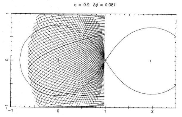
Figure 3.1: At each phase, when projected along the line of sight onto a given plane (here, and usually, the orbital plane) the limb of the secondary star forms an arc. Each point along such a ‘phase arc’ is eclipsed at the same moment. The figure shows various phase arcs at different orbital phases for $q=0.9$ and $\Delta\phi=0.081$. The axes are in units of the ${\rm L}_{1}$ distance. with the white dwarf at the origin. Figure from Horne (1985).

As previously discussed in § 1.6.3, the mass ratio—and hence the inclination—may be determined by comparing the bright spot light centres corresponding to the measured eclipse contact phases $\phi_{\rm{wi}}$ and $\phi_{\rm{we}}$ with the theoretical stream trajectories for different mass ratios $q$. This requires the assumption that the gas stream passes directly through the light centre of the bright spot. I constrain the light centre of the bright spot to be the point where the gas stream and outer edge of the disc intersect, so that the distance from the primary at which the gas stream passes through the light centre of the bright spot gives the outer disc radius $R_{\rm{d}}/a$. For data covering multiple eclipses, the uncertainties on these parameters may be determined from the root mean square (rms) variations of the measured contact phases.

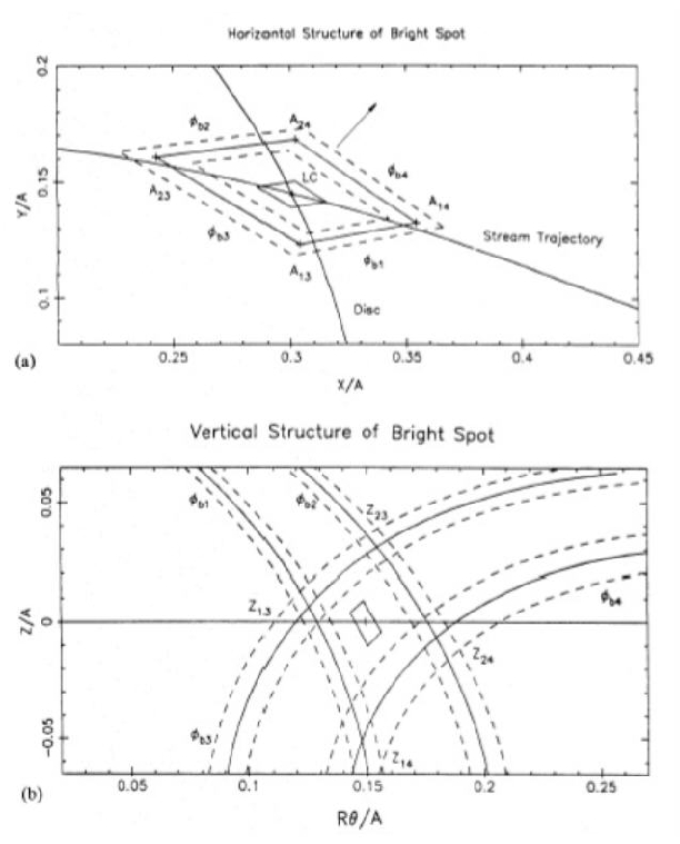
Figure 3.2: The horizontal and vertical structure of the bright spot of Z Cha for $q=0.1495$. The top panel (a) shows the region on the orbital $(x,y)$ plane on which the bright spot lies. The light centre of the bright spot LC is shown surrounded by a solid box corresponding to the rms variations in the phases of mid-ingress $\phi_{\rm bi}$ and mid-egress $\phi_{\rm be}$. Surrounding this is the solid box corresponding to the eclipse contact phases $\phi_{{\rm b}j}\ldots\phi_{{\rm b}k}$ (the vertices of which define $A_{jk}$) and their rms variations (dotted boxes). The accretion disc of radius $R_{\rm d}/a=0.334$ is also plotted, as is the stream trajectory. Panel (b) is similar, differing in that it shows the projection of the phase arcs onto the vertical cylinder of radius equal to that of the disc, $0.334a$, i.e. in the plane $(R\theta,z)$. $\theta$ increases in the direction of orbital motion and is zero at the line joining the centres of the two stars. Intersections of the phase arcs corresponding to the contact phases of the bright spot are labelled $Z_{jk}$. Figure from Wood et al. (1986).

The eclipse constraints on the structure of the bright spot can be used to determine upper limits on the angular size and the radial and vertical extent of the bright spot. Defining $A_{jk}$ and $Z_{jk}$ graphically in figure 3.2 as the positions of the intersections of the phase arcs $\phi_{{\rm b}j}$ and $\phi_{{\rm b}k}$ in the $(x,y)$ and $(R\theta,z)$ planes respectively, one can define

$$\Delta\theta = (\theta_{23}+\theta_{24}-\theta_{13}-\theta_{14})/2$$ (3.3a)

$$\Delta R_{\rm{d}} = (R_{24}+R_{14}-R_{23}-R_{13})/2$$ (3.3b)

$$\Delta Z = (H_{23}-H_{14})/2$$ (3.3c)

$$\Delta Z_{2} = H_{23},$$ (3.3d)

where $R_{jk}$ and $\theta_{jk}$ are the radius and azimuth of $A_{jk}$ and $H_{jk}$ the height of $Z_{jk}$ above the orbital plane. Equations 3.3a and 3.3b are defined as by Wood et al. (1986). Note that the definition of $\Delta Z$ in equation 3.3c differs slightly to that defined in Wood et al. (1986): this is in order to be more consistent with the definitions of $\Delta\theta$ and $\Delta R_{\rm d}$ in equations 3.3a and 3.3b. $\Delta Z_{2}$, defined in equation 3.3d, is identical to $\Delta Z$ as defined by Wood et al. (1986), and is included here for ease of comparison.

The eclipse constraints on the radius of the white dwarf can be used, together with the mass ratio and orbital inclination to determine the radius of the white dwarf. An alternative possibility is that the sharp eclipse is caused by a bright inner disc region or boundary layer surrounding the white dwarf like a belt. Another possibility is that the lower hemisphere of the white dwarf is obscured by an optically thick accretion disc, which would result in a larger white dwarf radius than that measured (see, for example, figure 4.6). The latter can be checked, as if the contact phases $\phi_{\rm wi}$ and $\phi_{\rm we}$ lie half-way through the white dwarf ingress and egress, the light distribution must be symmetrical.

The following analysis assumes that the eclipse is solely of a white dwarf. If the eclipse is actually of a belt and the white dwarf itself is not visible, then the white dwarf radius must be somewhat smaller than the radius of the belt. If the white dwarf does contribute significantly to the eclipsed light, then the white dwarf radius derived is actually an upper limit, so that the white dwarf mass determined from it is actually a lower limit (equation 1.15). The only way to verify the assumption that the central light source is the white dwarf alone is to measure the semi-amplitude of the radial velocity curve of the secondary star, $K_{2}$, and compare the resulting mass to that predicted by the photometric model. One could also check if this assumption is true using a longer baseline of quiescent observations, as one might expect eclipse timings of an accretion belt to be much more variable than those of a white dwarf. I note, however, that the white dwarf masses of OU Vir and XZ Eri, given in chapters 4 and 5 respectively, are consistent with the mean white dwarf mass of $0.69\pm 0.13\;{\rm M}_{\odot}$ for CVs below the period gap (Smith & Dhillon, 1998). Although the white dwarf in DV UMa is unusually massive, the assumption that we are observing the white dwarf and not the boundary layer around the primary cannot cause this, as the white dwarf mass derived would be in this case a lower limit. Also, Baptista et al. (2000) point out that in short-period dwarf novæ (specifically OY Car, Z Cha and HT Cas; Wood & Horne, 1990) like OU Vir, XZ Eri and DV UMa the boundary layer is faint (or absent), whereas longer-period dwarf novæ such as IP Peg (Wood & Crawford, 1986) and EX Dra (Baptista et al., 2000) usually have detectable boundary layers. As an illustrative example, in the case of EX Dra, Baptista et al. (2000) conclude that the white dwarf is surrounded by an extended boundary layer on the basis of the implausibly low white dwarf masses implied by assuming otherwise and the observed variability of both the flux and duration of the primary eclipse. Throughout this thesis I assume that the central eclipsed object is indeed a white dwarf.

Light curve deconvolution

Once the white dwarf eclipse contact phases have been found, the white dwarf light curve can be reconstructed and subtracted from the overall light curve, as illustrated in figure 3.3. The procedure is as follows. The white dwarf flux is assumed to be zero between the contact phases $\phi_{2}$ and $\phi_{3}$, as here the white dwarf is totally eclipsed. The derivative between the contact phases is then numerically integrated. The white dwarf flux is assumed to be constant outside eclipse, and is determined from the mean of the integrated flux at contact phases $\phi_{1}$ and $\phi_{4}$. The result is symmetrized about phase zero, and smoothed to obtain a noise-free estimate of the white dwarf light curve. This can then be subtracted from the overall light curve to give the light curve of the bright spot and disc. The white dwarf flux thus determined can be used to determine its temperature and distance (see § 3.6).

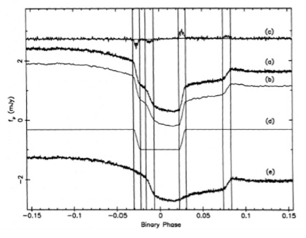
Figure 3.3: Deconvolution of the white dwarf light curve of Z Cha from the mean light curve. (a) shows the original mean light curve; (b) the smoothed light curve, offset downwards by 0.5 mJy; (c) the derivative of the smoothed light curve, with a spline fit to phases outside ingress and egress superimposed, both offset upwards by 2.75 mJy and multiplied by a factor of 10; (d) the reconstructed white dwrf eclipse, offset downwards by 1 mJy; and (e) the original mean light curve after subtraction of the white dwarf light curve, offset downwards by 3 mJy. The vertical lines mark the contact phases of the white dwarf and bright spot. Figure from Wood et al. (1986).

3.3 Lfit method

Another way of determining the system parameters is to use a physical model of the binary system to calculate eclipse light curves for each of the various components. I used the technique developed by Horne et al. (1994) and described in detail therein. This model assumes that the eclipse is caused by the secondary star, which completely fills its Roche lobe. A few changes were necessary in order to make the model of Horne et al. (1994) suitable for my data. The most important of these was the fitting of the secondary flux, prompted by the detection of a significant amount of flux from the secondary in the i^′ band of DV UMa. The secondary flux is very small in all the other bands.

The 10 parameters that control the shape of the light curve are as follows:

1. The mass ratio $q$.

2. The eclipse phase full-width at half-depth $\Delta\phi$.

3. The outer disc radius $R_{\rm{d}}/a$.

4. The white dwarf limb darkening coefficient $U_{1}$.

5. The white dwarf radius $R_{1}/a$.

6. The bright spot scale $SB/a$. The bright spot is modelled as a linear strip passing through the intersection of the gas stream and disc. The relative intensity distribution along this strip is given by $(X/SB)^{2}e^{-X/SB}$, where $X$ is the distance along the strip, the maximum being at the intersection of the bright spot and disc, at $X=2SB$. The relative intensity $I$ of the bright spot is then modulated according to the orbital phase by a sine function. For DV UMa this function was

   $$I=\left\{\begin{array}[]{ll}\sin(\theta_{\rm{B}}+\phi)&\mbox{if $\sin(\theta_{\rm{B}}+\phi)>0$}\\ 0&\mbox{otherwise}\end{array}\right.,$$ (3.4a)

   where $$\theta_{\rm{B}}$$ is as defined below. For XZ Eri a better fit was achieved using

   $$I=\left\{\begin{array}[]{ll}\sin^{2}(\theta_{\rm{B}}+\phi)&\mbox{if $\sin(\theta_{\rm{B}}+\phi)>0$}\\ 0&\mbox{otherwise}\end{array}\right..$$ (3.4b)

7. The line along which, on the edge of the disc, the bright spot lies is tilted by an angle $\theta_{\rm{B}}$, measured relative to the line joining the white dwarf and the secondary star. The bright spot does not, therefore, necessarily emit its anisotropic light (see below) in a direction normal to the edge of the accretion disc. This allows adjustment of the phase of the orbital hump.

8. The fraction of bright spot light which is isotropic $f_{\rm{iso}}$. The bright spot emits a fraction of its light isotropically, in all directions, and the remainder anisotropically, in a direction which determines the phase of the orbital hump maximum.

9. The disc exponent $b$, describing the power law of the radial intensity distribution of the disc. The relative intensity $I$ at a radius $R$ of the disc is $I\propto R^{b+1}$.

10. A phase offset $\phi_{0}$.

The light curve $D(\phi)$ was modelled as a sum of multiple components (the white dwarf, bright spot, accretion disc and red dwarf), the contribution of the first three of which can vary with the orbital phase $\phi$:

$$M(\phi)=\sum_{i=1}^{n}L_{i}(\phi),$$ (3.5)

where $M(\phi)$ is the model flux at phase $\phi$ and $L_{i}(\phi)$ is the flux of component $i$ at phase $\phi$. Fitting of ellipsoidal variations made no significant improvement to the overall fit, so I have assumed the flux from the secondary star to be constant. The amoeba algorithm (downhill simplex; Press et al., 1986) was used to adjust selected parameters to find the best fit. The algorithm attempts to minimise $\chi^{2}$, the usual goodness-of-fit statistic:

$$\chi^{2}=\sum_{j=1}^{n}\left(\frac{D_{j}-M_{j}}{\sigma_{j}}\right)^{2}.$$ (3.6)

It is often useful to define a reduced $\chi^{2}$,

$$\chi^{2}_{\rm R}=\frac{\chi^{2}}{n-\nu},$$ (3.7)

where $\nu$ is the number of degrees of freedom. At each evaluation of the function $M(\phi)$ the light curves of the individual components were scaled using a linear regression, the shape of each light curve being set by the values of the parameters at that time. A positivity constraint was imposed: whenever a negative flux was found for a component, the flux of that component was set to zero and the fit was repeated to determine the flux for the other components. The procedure did not iterate to $\chi^{2}_{\rm R}=1$ due to the presence of flickering and other variability in the light curve not allowed for in the model. Consequently, the algorithm was run until the parameters output no longer changed significantly between iterations (i.e. the parameter change was less than the typical uncertainty on each parameter; see below). Typically, a minimum of $10\,000$ iterations were performed to produce the parameters presented in this thesis.

The $1\sigma$ error on an individual parameter of a M-dimensional model fit is given (Lampton et al., 1976) by the perturbation of that parameter necessary to increase the $\chi^{2}$ of the fit by 1, i.e.

$$\chi^{2}-\chi_{\rm{min}}^{2}=\Delta\chi^{2}=1.$$ (3.8)

This is, of course, equivalent to finding the root of

$$f(\chi^{2})=\chi^{2}-\chi_{\rm{min}}^{2}-1.$$ (3.9)

The procedure I employed to determine the errors on each parameter was as follows. I perturbed the parameter of interest from its best fit value by an arbitrary amount (initially 5 per cent) and re-optimised the rest of them (holding the parameter of interest, and any others originally kept constant, fixed). The amoeba algorithm was allowed to iterate for $2100$ iterations, then the new value of $\chi^{2}$ was computed. If the root was not bracketed by the two values of $\chi^{2}$, i.e. $\chi^{2}-\chi_{\rm{min}}^{2}<1$, then the perturbation was increased by a factor of $4$ until it was. A bisection method (Press et al., 1986) was then used to find the value of the parameter in question which gave the root of equation 3.9, with the value of $\chi^{2}$ at each step being computed as described previously in this paragraph. The difference between the final, perturbed, value of the parameter and its best fit value gave the $1\sigma$ error on that parameter.

3.4 Comparing the derivative and lfit methods

The methods discussed in the previous two sections, the derivative and lfit techniques, were compared with each other using fake light curves.

Fake, noise-free light curves were kindly produced by Dr. Chris Watson using his rochey code to specifications set out by myself. All other work in this section was conducted by myself under the supervision of Dr. Vik Dhillon. Gaussian noise was then added to the resultant light curve. The errors were of the form

$$\sigma_{{\rm i}}=E\sqrt{f_{i}f_{2}}+\frac{Ef_{2}}{10},$$ (3.10)

where $E$ is an arbitrary number controlling the fractional error, $f_{i}$ the flux on datapoint $i$ and $f_{2}$ the flux on the second datapoint (chosen arbitrarily because it is out of eclipse and not contaminated by the orbital hump). The first term scales the error with the square root of the flux, as expected for shot noise, with the $\sqrt{f_{2}}$ term ensuring that the signal-to-noise ratio of the second datapoint is $\sim\frac{1}{E}$. The final term prevents the error on a zero flux point being zero, which is both unphysical and causes coding problems (mainly with dividing by zero). The noise added to the data was

$$f_{i}=f_{i}+R\sigma_{i},$$ (3.11)

where $R$ is a normally-distributed random number with zero mean and unit variance. Flickering was modelled by adding additional (Gaussian) noise to the light curve but not increasing the errors. For all the fake light curves used in this section, $E=0.04$ for the addition of both noise and flickering. The amplitude of the flickering scaled with the flux level so that flickering during mid-eclipse was much less than that out of eclipse. This is designed to reproduce the real behaviour of flickering, which is observed to be greatly reduced during eclipse (e.g. Patterson, 1981; Bruch, 2000; Baptista & Bortoletto, 2004).

The parameters used to produce the fake light curves used for the comparison of the derivative and lfit methods are given in table 3.1. The properties of the various fake light curves I used are given below:

1. A ‘normal’ light curve, with the ingress and egress of the white dwarf and bright spot clear and distinct.

2. As 1, but with the ingress of the white dwarf and bright spot merged together, as seen for IP Peg (whose parameters have been used to produce this light curve).

3. The aim of these light curves is to investigate the case of the compact objects (the white dwarf and bright spot) being relatively faint. I would expect that if the level of noise and/or flickering becomes greater than the amplitude of the eclipse, then determination of the system parameters would become difficult/impossible.

   1. Faint white dwarf.

   2. Faint bright spot.

4. The aim of these light curves is to investigate what happens to the estimated parameters when the assumption that the bright spot lies at the intersection of the accretion disc and gas stream is broken. To this end:

   1. The bright spot is ahead of the impact region.

   2. The bright spot is behind the impact region.

5. These light curves have different accretion disc radii to check that both techniques are effective over a range of parameters.

   1. A smaller disc radius, of $0.25a$.

   2. A larger disc radius, of $0.36a$.

The model used to produce the fake light curves was a grid of the accretion disc and secondary star, with each element in the grid array having an adjustable intensity. The secondary star was assumed to fill its Roche lobe, so the surface of the secondary star is defined by the critical potential. The visibility of each grid element, or tile, was tested at a given phase for a given mass ratio and orbital inclination, and a light curve built up in this manner. The grid used for model 1 (described in table 3.1) is illustrated in figure 3.4. The disc has a height of $0.0002a$ above the orbital plane, with the rim of the disc being subdivided into tiles which can be used to model the orbital hump. The white dwarf was modelled by increasing the intensity of the disc tiles at the centre of the disc. The bright spot was modelled by a disc rim only. Modelling the bright spot as a combination of the disc rim and tiles in the outer annulus of the disc led to incorrect determinations of the disc radius and mass ratio. This is because the disc rim is at the outer radius of the accretion disc, whereas, since a tile is only flagged as eclipsed when its centre is eclipsed, the radius of the outer annulus is slightly (the difference being half the width of the outer annulus) smaller than the radius of the disc rim. The intensity of the secondary star was set to zero in all models, as it is usually very faint in faint short-period dwarf novæ.

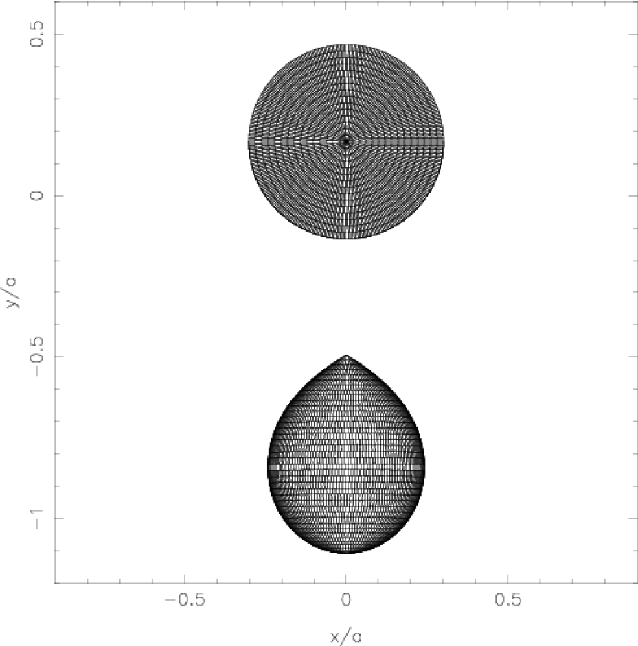
Figure 3.4: The model grid used to produce the fake data for comparing the results of the derivative and lfit techniques. The origin is at the centre of mass; otherwise the co-ordinate system is as described in chapter 1. Figure by Dr. Chris Watson.

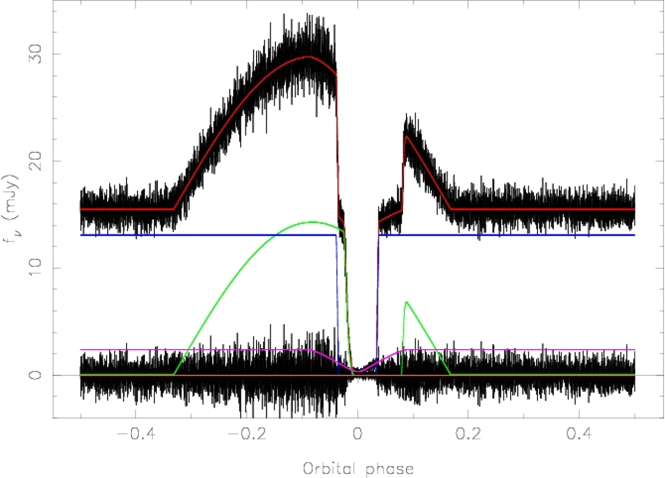
Figure 3.5: Fake light curve produced as described in the text using the parameters given in table 3.1 for model 1.

The parameters recovered from the various models are given in tables 3.2 and 3.3 for the lfit and derivative techniques, respectively. The light curve fits from the lfit program are shown in figures 3.5–3.12.

Table 3.1: The input parameters of the fake light curves used for comparison of the derivative and lfit methods. The white dwarf has in all cases a radius $R_{1}=0.02a$ and the bright spot $R_{\rm{bs}}=0.04a$. The disc radius is $R_{\rm{d}}=0.3a$ for all the light curves except models 5a and 5b. The relative contributions (in arbitrary units) of the white dwarf (WD), bright spot (BS), accretion disc (AD) and red dwarf (RD) are also given.

					Bright spot position		Flux (arbitrary units)
Model	$q$	$i(\deg)$	$\Delta\phi$	$P$ (sec)	$x/a$	$y/a$	WD	BS	AD	RD
1	0.20	$85.0^{\circ}$	0.0725	7200	0.2663	0.1381	13.00678	14.29689	2.45069	0
2	0.43	$82.2^{\circ}$	0.0863	13669	0.2826	0.1006	13.9795	11.6358	3.79294	0
3a	0.20	$85.0^{\circ}$	0.0725	7200	0.2663	0.1381	2.1678	14.29689	2.45069	0
3b	0.20	$85.0^{\circ}$	0.0725	7200	0.2663	0.1381	13.00678	2.3828	2.45069	0
4a	0.20	$85.0^{\circ}$	0.0725	7200	0.2472	0.1700	13.00677	14.30843	2.45069	0
4b	0.20	$85.0^{\circ}$	0.0725	7200	0.2828	0.1000	13.00677	14.08273	2.45069	0
5a	0.20	$85.0^{\circ}$	0.0725	7200	0.2006	0.1491	12.91617	11.92371	1.6998	0
5b	0.20	$85.0^{\circ}$	0.0725	7200	0.3396	0.1195	12.92509	7.42059	3.51082	0

Table 3.2: Reconstructed parameters from lfit.

	Model number
Parameter	1	2	3
			a	b
Error (per cent)	4	4	4	4
Flickering
(per cent)	4	4	4	4
Inclination $i$	$84.8^{\circ}\pm 0.1^{\circ}$	$81.6^{\circ}\pm 0.1$	$84.77^{\circ}\pm 0.03^{\circ}$	$86.2^{\circ}\pm 0.4^{\circ}$
Mass ratio $q$	$0.2035$	$0.455$	$0.20579$	$0.181$
	$\pm 0.0010$	$\pm 0.004$	$\pm 0.00014$	$\pm 0.006$
Eclipse phase	$0.07255$	$0.08629$	$0.072643$	$0.07252$
width $\Delta\phi$	$\pm 0.00005$	$\pm 0.00004$	$\pm 0.00015$	$\pm 0.00005$
Outer disc	$0.2983$	$0.2912$	$0.29558$	$0.3215$
radius $R_{\rm{d}}/a$	$\pm 0.0013$	$\pm 0.0023$	$\pm 0.00026$	$\pm 0.0004$
White dwarf
limb	$0.5$	$0.5$	$0.5$	$0.5$
darkening $U_{\rm{1}}$
White dwarf	$0.0132$	$0.0106$	$0.0135$	$0.01376$
radius $R_{1}/a$	$\pm 0.0003$	$\pm 0.0003$	$\pm 0.0006$	$\pm 0.00029$
Bright spot	$0.01179$	$0.01135$	$0.01169$	$0.0123$
scale $SB/a$	$\pm 0.00018$	$\pm 0.00026$	$\pm 0.00006$	$\pm 0.0006$
Bright spot	$119.42^{\circ}$	$111.51^{\circ}$	$119.41^{\circ}$	$119.3^{\circ}$
orientation $\theta_{\rm{B}}$	$\pm 0.08^{\circ}$	$\pm 0.16^{\circ}$	$\pm 0.012^{\circ}$	$\pm 0.5^{\circ}$
Isotropic flux	$0.0017$	$0.009$	$0.0006$	$0.013$
fraction $f_{\rm iso}$	$\pm 0.0028$	$\pm 0.008$	$\pm 0.0013$	$\pm 0.015$
Disc exponent $b$	$0.16\pm 0.12$	$0.10\pm 0.3$	$0.10\pm 0.18$	$-0.49\pm 0.12$
Phase offset $\phi_{0}$	$0$	$0$	$0$	$0$
$\chi^{2}$ of fit	$14498$	$25940$	$18688$	$13127$
Number of
datapoints $\nu$	$7199$	$13668$	$7199$	$7199$
Flux
(arbitrary units)
White dwarf	$13.08\pm 0.04$	$14.039\pm 0.038$	$2.199\pm 0.022$	$12.94\pm 0.03$
Accretion disc	$2.37\pm 0.04$	$3.59\pm 0.04$	$2.422\pm 0.028$	$2.50\pm 0.03$
Secondary	$0$	$0.042\pm 0.010$	$0.006\pm 0.008$	$0$
Bright spot	$14.288\pm 0.026$	$12.094\pm 0.024$	$14.289\pm 0.011$	$2.395\pm 0.020$

Table 3.2: Continued. Reconstructed parameters from lfit. No error estimates could be determined for some parameters of model 4a, since the fit became unphysical if left to iterate to convergence.

	Model number
Parameter	4		5
	a	b	a	b
Error (per cent)	4	4	4	4
Flickering
(per cent)	4	4	4	4
Inclination $i$	$89.7^{\circ}$	$77.3^{\circ}\pm 0.1^{\circ}$	$84.4^{\circ}\pm 0.1^{\circ}$	$85.6^{\circ}\pm 0.2^{\circ}$
Mass ratio $q$	$0.157$	$0.5254$	$0.2128$	$0.1902$
		$\pm 0.0024$	$\pm 0.0013$	$\pm 0.0020$
Eclipse phase	$0.0725$	$0.07258$	$0.07259$	$0.07255$
width $\Delta\phi$		$\pm 0.00005$	$\pm 0.00006$	$\pm 0.00006$
Outer disc	$0.2908$	$0.2635$	$0.2439$	$0.3629$
radius $R_{\rm{d}}/a$	$\pm 0.0011$	$\pm 0.0007$	$\pm 0.0007$	$\pm 0.0008$
White dwarf
limb	$0.5$	$0.5$	$0.5$	$0.5$
darkening $U_{\rm{1}}$
White dwarf	$0.01420$	$0.01137$	$0.0174$	$0.0137$
radius $R_{1}/a$	$\pm 0.00026$	$\pm 0.00021$	$\pm 0.0003$	$0.0004$
Bright spot	$0.0160$	$0.01448$	$0.00928$	$0.00612$
scale $SB/a$	$\pm 0.0003$	$\pm 0.00016$	$\pm 0.00016$	$0.00020$
Bright spot	$126.95^{\circ}$	$111.08^{\circ}$	$127.94^{\circ}$	$110.76^{\circ}$
orientation $\theta_{\rm{B}}$	$\pm 0.09^{\circ}$	$\pm 0.08^{\circ}$	$\pm 0.11^{\circ}$	$\pm 0.16$
Isotropic flux	$0.030$	$0.0091$	$0.0013$	$0.018$
fraction $f_{\rm iso}$	$\pm 0.003$	$\pm 0.0026$	$\pm 0.0027$	$\pm 0.006$
Disc exponent $b$	$-0.70\pm 0.23$	$0.2\pm 0.4$	$-0.93\pm 0.13$	$-0.08\pm 0.15$
Phase offset $\phi_{0}$	$0$	$0$	$0$	$0$
$\chi^{2}$ of fit	$16399$	$14523$	$14385$	$13538$
Number of
datapoints $\nu$	$7199$	$7199$	$7199$	$7199$
Flux
(arbitrary units)
White dwarf	$12.71\pm 0.06$	$13.28\pm 0.05$	$12.86\pm 0.04$	$12.97\pm 0.06$
Accretion disc	$2.14\pm 0.08$	$1.79\pm 0.06$	$1.76\pm 0.04$	$3.25\pm 0.09$
Secondary	$0.175\pm 0.017$	$0.273\pm 0.013$	$0$	$0.09\pm 0.03$
Bright spot	$14.658\pm 0.025$	$14.303\pm 0.028$	$11.898\pm 0.023$	$7.78\pm 0.03$

Table 3.3: Reconstructed parameters from the derivative method.

	Model number
Parameter	1	2	3
			a	b
Error (per cent)	4	4	4	4
Flickering (per cent)	4	4	4	4
Inclination $i$	$84.8^{\circ}$	$81.9^{\circ}$	$85.4^{\circ}$	$88.0^{\circ}$
Mass ratio $q$	0.206	0.470	0.200	0.169
$\Delta\phi$	0.072649	0.088308	0.073344	0.073205
$\Delta R_{{\rm d}}/a$	0.0326	0.0692	0.0314	0.1589
$\Delta\theta$	$9.4^{\circ}$	$11.8^{\circ}$	$16.1^{\circ}$	$12.5^{\circ}$
$\Delta Z/a$	–	–	–	–
$\Delta Z_{2}/a$	0.0347	0.0586	0.0539	0.0987
$R_{{\rm d}}/a$	0.3043	0.2944	0.3076	0.3394
$\theta$	$26.3^{\circ}$	$19.4^{\circ}$	$26.3^{\circ}$	$23.5^{\circ}$

Table 3.3: Continued. Reconstructed parameters from the derivative method.

	Model number
Parameter	4		5
	a	b	a	b
Error (per cent)	4	4	4	4
Flickering (per cent)	4	4	4	4
Inclination $i$	–	$77.3^{\circ}$	$86.8^{\circ}$	$85.9^{\circ}$
Mass ratio $q$	$<0.164$	0.53	0.195	$0.185$
$\Delta\phi$	0.073344	0.072927	0.075149	0.072510
$\Delta R_{{\rm d}}/a$	–	0.0332	0.0293	0.0406
$\Delta\theta$	–	$21.2^{\circ}$	$21.5^{\circ}$	$5.1^{\circ}$
$\Delta Z/a$	–	0.0346	–	0.0515
$\Delta Z_{2}/a$	–	0.0296	0.0421	0.0549
$R_{{\rm d}}/a$	–	0.2369	0.2460	0.3633
$\theta$	–	$26.7^{\circ}$	$37.9^{\circ}$	$19.6^{\circ}$

The errors on the parameters as determined by lfit are clearly too small when compared to the input parameters given in table 3.1. As such, they likely represent the reproducibility of the fit to the data, rather than the standard deviation from the true values. It is probable that there is a systematic error present between the model used to generate the light curves and the model used to reconstruct them. This highlights the fact that any such model-fitting approach to the determination of the system parameters will suffer from the applicability of the model: that is, one does not know how far from reality the model deviates. One such likely discrepancy is in the form of the bright spot intensity distribution. Lfit models this in the eminently reasonable form given in § 3.3. If the intensity distribution of the bright spot differs from this, however, then a systematic error will be introduced into the estimate of the mass ratio due to the position of the centre-of-light of the bright spot differing from that expected. Another possible explanation of the small errors is that they may be due to the program having difficulty in iterating to $\chi^{2}_{{\rm min}}$ during the bisection used to determine the errors.

I did not estimate uncertainties for the parameters produced by the derivative technique, as first, the dominant source of error is likely to be systematic differences between the models used to produce and analyse the light curves and second, due to the prohibitive amount of time it would have taken to produce and analyse the multiple light curves necessary to determine the rms variations in the contact phases.

Models 1, 2, 3a, 4b, 5a, 5b and arguably 3b were satisfactorily reconstructed by both the lfit and derivative methods. Model 4a was found to produce an unphysical light curve with the derivative technique, since the constraints placed upon the eclipse phase width $\Delta\phi$ (by the white dwarf eclipse width) and the mass ratio $q$ (by the positions of the bright spot ingress and egress) were not consistent with an orbital inclination $i\leq 90^{\circ}$. The lfit method produced a very small mass ratio (as might be expected, since a reduction in $q$ moves the path of the gas stream further from the white dwarf), but also a very high orbital inclination, which meant that the solution found by the iterative procedure became unphysical if left to iterate towards an optimum result. Model 4b was reconstructed with a lower orbital inclination, which was caused by the model fitting a larger mass ratio in order to place the bright spot at the correct location. Models 5a and 5b were adequately reconstructed by each technique, confirming the reliability of both over a range of different accretion disc radii.

Comparison of the recovered parameters for models 3a and 3b leads to the conclusion that the visibility of the bright spot is more important than the visibility of the white dwarf. This is perhaps due to the fact that the white dwarf eclipse is symmetrical, so the twin constraints of ingress and egress lead it to being much less susceptible to noise in the data than the a symmetric light curve of the bright spot. The times of ingress and egress of the bright spot are dependent on more parameters than those of the white dwarf: the bright spot times depend on the mass ratio, the disc radius, the phase offset and the orbital inclination, as opposed to the eclipse phase width, the phase offset and the orbital inclination for the white dwarf.

The fluxes recovered for each component by the lfit method were generally in good agreement with the input fluxes, as can be seen by comparison of the relevant figures in tables 3.1 and 3.2. The largest discrepancies occur for models 4a and 4b, as might be expected, since one of the basic assumptions of the method is deliberately broken for both these models. Again, it appears that systematic errors frequently dominate, a fact that should be borne in mind when fluxes derived in this way are used.

In conclusion, both techniques reproduced the system parameters well in all of the realistic light curves (models 1, 2, 3a, 3b, 5a and 5b). The parameters for model 3b were rather less accurate, as the bright spot was to some extent lost amongst the noise. The errors determined by the lfit method (by increasing $\chi^{2}$ by 1) were too small, suggesting that systematic errors introduced by differences between the assumed model and the real case are the dominant source of error. Agreement between the two methods was good for all the models investigated. Breaking the assumption that the bright spot was at the intersection of the gas stream and accretion disc’s outer edge had predictable results: placing it ahead of the intersection led to too small a mass ratio; behind too large a mass ratio.

These two techniques were also compared using real data, as discussed in § 5.3.3.

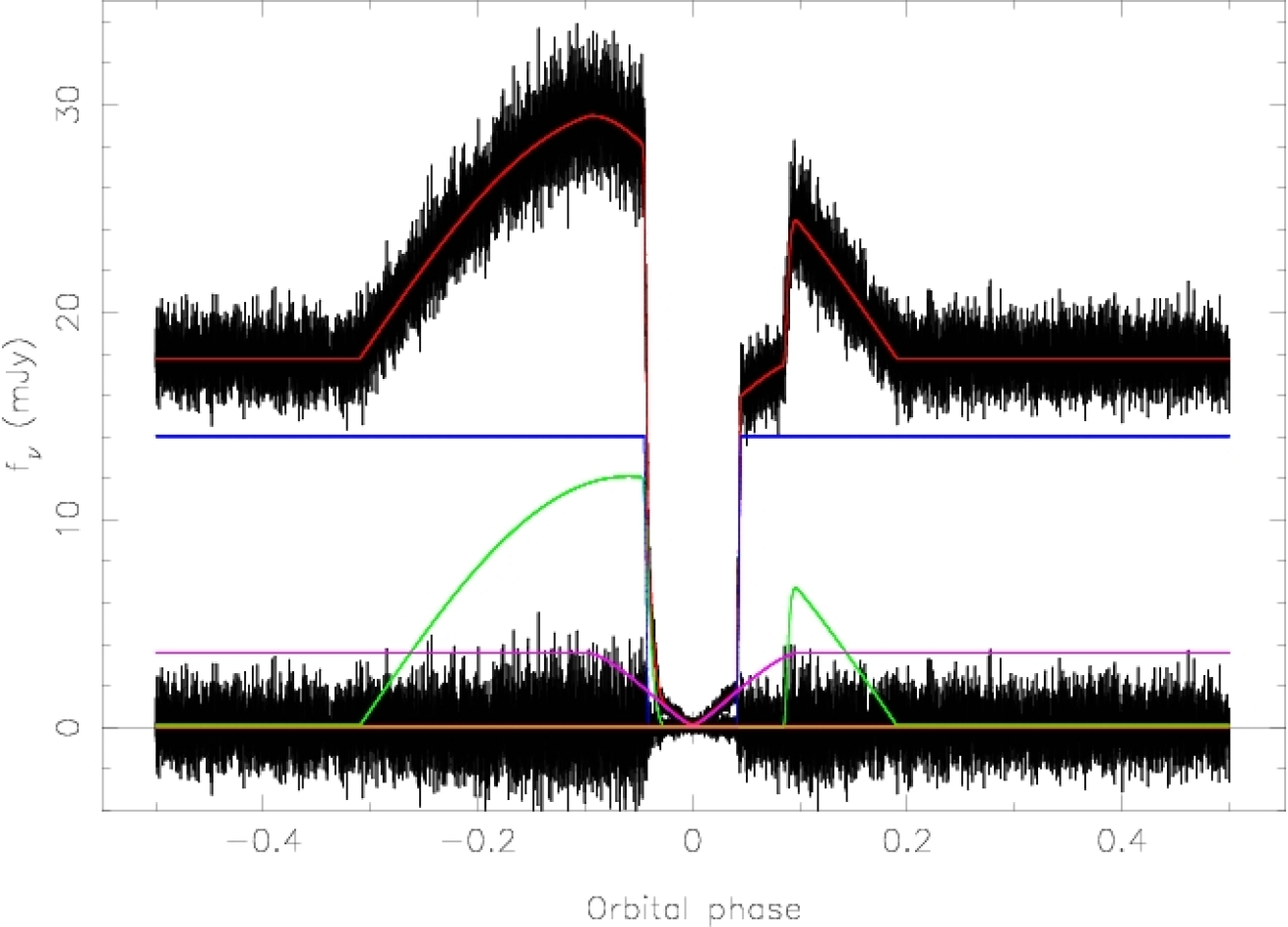
Figure 3.6: Fake light curve produced as described in the text using the parameters given in table 3.1 for model 2.

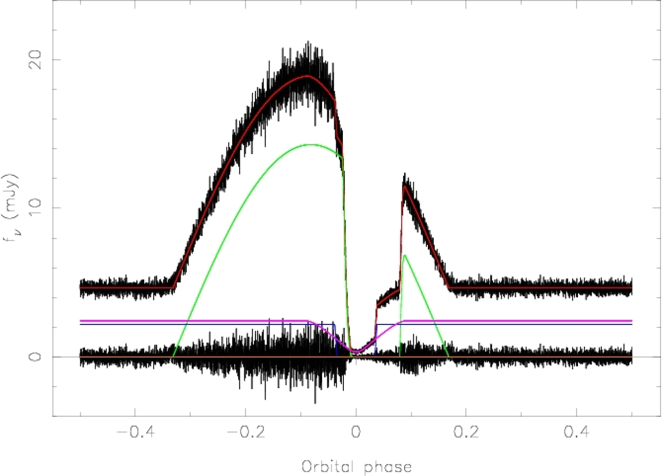
Figure 3.7: Fake light curve produced as described in the text using the parameters given in table 3.1 for model 3a.

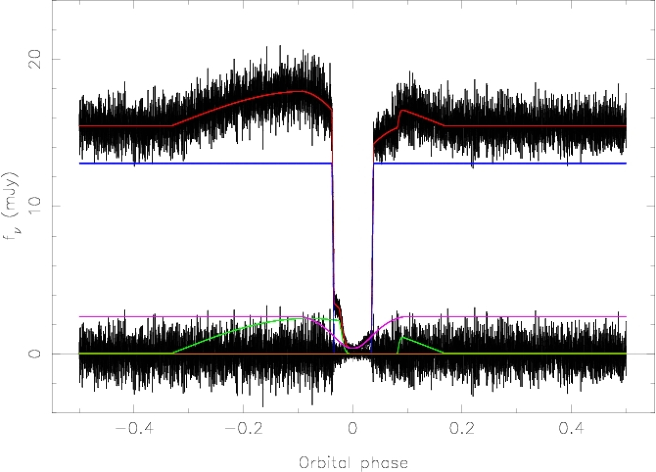
Figure 3.8: Fake light curve produced as described in the text using the parameters given in table 3.1 for model 3b.

Figure 3.9: Fake light curve produced as described in the text using the parameters given in table 3.1 for model 4a.

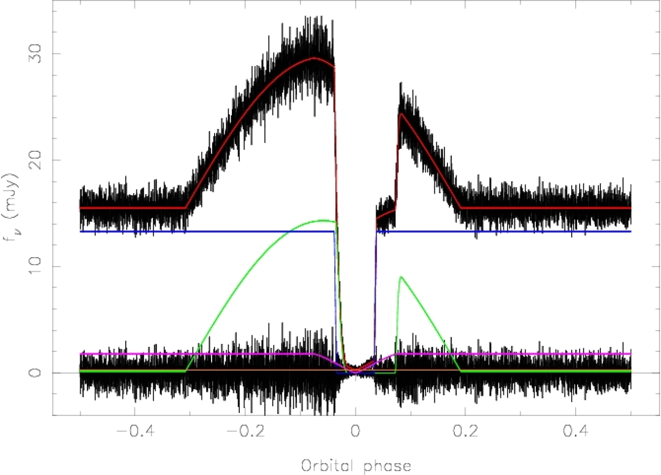
Figure 3.10: Fake light curve produced as described in the text using the parameters given in table 3.1 for model 4b.

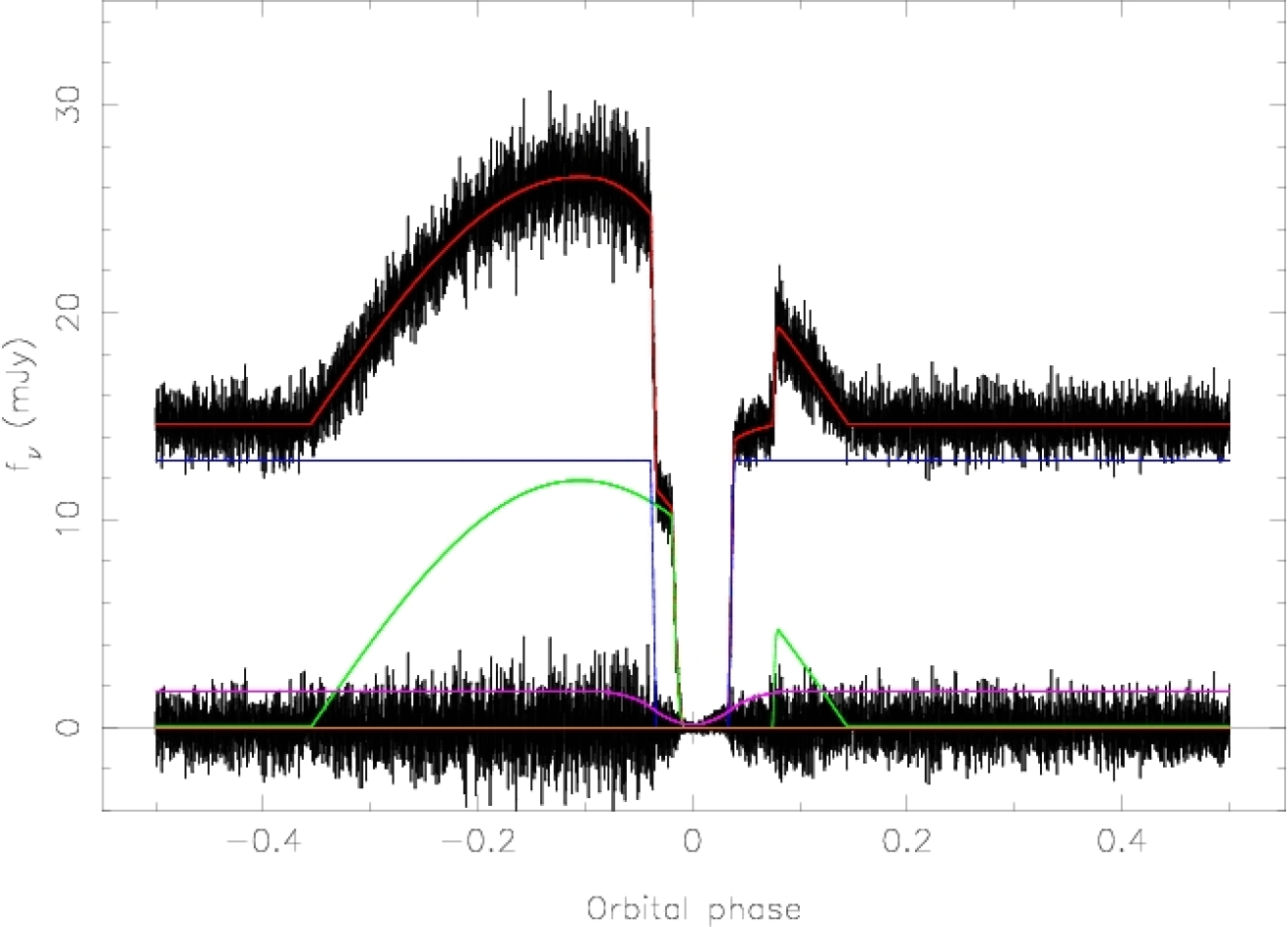
Figure 3.11: Fake light curve produced as described in the text using the parameters given in table 3.1 for model 5a.

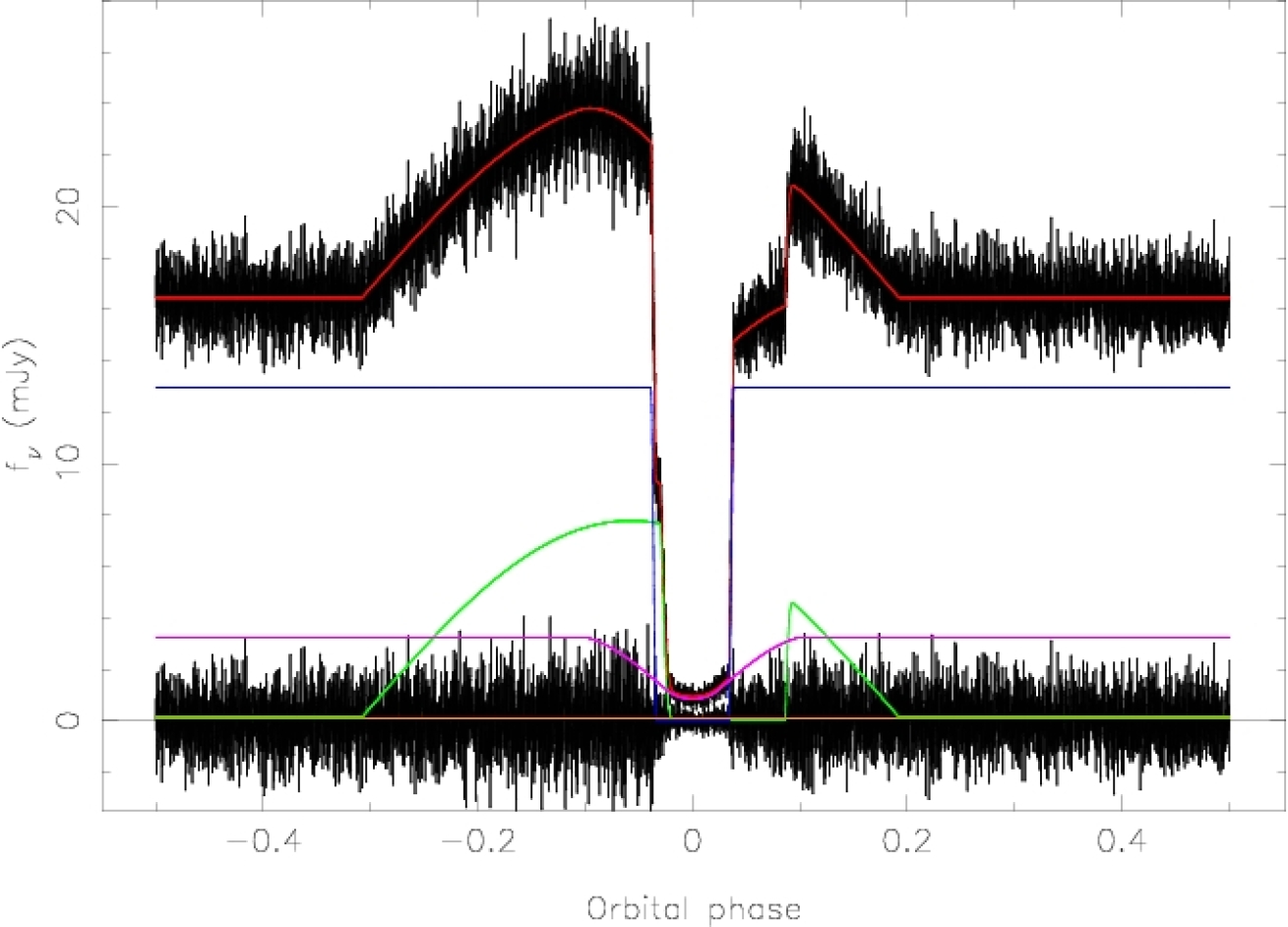
Figure 3.12: Fake light curve produced as described in the text using the parameters given in table 3.1 for model 5b.

3.5 Mass determination

The derivative and lfit techniques yield the system parameters relative to the orbital separation (or the L₁ distance). To determine the absolute system parameters I have used the Nauenberg mass-radius relation for a cold, non-rotating white dwarf (equation 1.15). If one sets $R_{1}/a=y$, Kepler’s third law (equation 1.1) can be rewritten in terms of the parameters $R_{1}$ and $y$, giving another restriction on the white dwarf radius:

$$R_{1}=y\left(\frac{GM_{1}(1+q)P^{2}_{\rm{orb}}}{4\pi^{2}}\right)^{\frac{1}{3}}.$$ (3.12)

Equations 1.15 and 3.12 can be easily solved to give the system parameters. The secondary radius $R_{2}$ can be calculated by approximating it to the volume radius of the Roche lobe (equation 1.4).

As the Nauenberg (1972) mass-radius relation assumes a cold white dwarf, I have attempted to correct this relation to the approximate temperature given by a fit to the deconvolved white dwarf fluxes (see below). Wood et al. (1989a) and Koester & Schönberner (1986) note that the radius of a white dwarf at $10^{4}$ K is about 5 per cent larger than a cold white dwarf. To correct to the appropriate temperature from $10^{4}$ K the white dwarf cooling curves of Wood (1995) have been used.

3.6 White dwarf model atmospheres

The temperature and distance of the white dwarf component can be determined by fitting the fluxes from three filters to the spectrum of a blackbody or model atmosphere.

The expected flux $f$ from a blackbody $B_{\nu}(\lambda,T)$ in a passband with transmission function $P(\lambda)$ is (e.g. Wood et al., 1989a)

$$f=\frac{\int P(\lambda)B_{\nu}(\lambda,T)d\lambda/\lambda}{\int P(\lambda)d\lambda/\lambda}\cdot\frac{\pi R^{2}_{1}}{D^{2}},$$ (3.13)

where $D$ is the distance to the star. By fitting a blackbody function to the white dwarf flux in each passband the white dwarf temperature $T_{1}$ and distance can be determined. As a white dwarf spectrum is one of the closest astronomical approximations to a blackbody, this procedure is reasonable.

The white dwarf fluxes were also fitted to the hydrogen-rich, $\log g=8$ white dwarf model atmospheres of Bergeron et al. (1995) by $\chi^{2}$ minimisation. The colour indices quoted therein were converted to the SDSS system using the observed transformations of Smith et al. (2002). This procedure determined the temperature of the white dwarf but not the distance, since the absolute magnitude (and hence the distance) is much more heavily dependent on the exact value of $\log g$ than the colours (which give the temperature). This latter method, however, will determine the white dwarf temperature more accurately than a blackbody fit, as it will allow, for example, for the Balmer jump in the white dwarf spectrum.

3.7 Eclipse mapping

In § 1.5.1 I discussed various theoretical models and predicted properties of accretion discs, and alluded to a technique whereby the intensity distribution across the disc could be uncovered. This technique, called eclipse mapping, is the subject of this section.

The eclipse mapping method was developed by Horne (1985). It enables the light distribution across the disc (including the contributions of the white dwarf and bright spot) of eclipsing systems to be mapped. The shape of the eclipse produced by the occultation of the accretion disc by the red dwarf depends on the light distribution across the disc. Unfortunately, as the eclipse light curve is one-dimensional, and the light distribution across the disc is two-dimensional (in the approximation of a flat disc), the solution is not unique. One possible solution to this is to use a model-fitting approach, but this has the obvious disadvantage that it is model-dependent. This problem becomes more acute when it is considered that our present knowledge of accretion disc physics is incomplete. The departure of accretion discs in CVs from axi-symmetry, due to the impact of the gas stream with the edge of the disc, provide another problem for model-fitting procedures.

The above concerns naturally lead to the eclipse-mapping approach. In this method, the intensity at each point of the accretion disc is an independent parameter. In the simplest implementation of the method, the disc is modelled as a simple Cartesian grid, co-rotating with the binary system. In this form, the eclipse mapping method makes three basic assumptions:

1. The secondary star fills its Roche-lobe. There is ample evidence (e.g. ellipsoidal variations from the distorted secondary star; Allan et al., 1996) for mass transfer via Roche-lobe overflow (the very presence of the accretion disc and bright spot imply it), so this assumption seems reasonably valid.

2. The intensity distribution is two-dimensional; it is constrained to the orbital plane. Rutten (1998) found that this is a good assumption provided that the inner disc regions are not obscured by the disc rim. The opening angles of accretion discs in CVs are typically $\sim 5^{\circ}$ (for example, the disc in the SW Sex star DW UMa has an opening angle of $\geq 8^{\circ}$; Knigge et al., 2000), so this assumption is (reasonably) valid for orbital inclinations $i\lesssim 85^{\circ}$.

3. The emission is phase-independent (apart from the eclipse by the secondary star). This last assumption is the most problematic. Many CVs have orbital humps due to anisotropic radiation from the bright spot, which violates this assumption. In the following section I discuss how this may be accounted for.

The eclipse-mapping technique has since been further developed to allow spectral eclipse mapping (Rutten et al., 1993, 1994), modelling of a three-dimensional accretion disc (Rutten, 1998), fitting of multi-colour light curves by physical properties of a model disc (so-called physical parameter eclipse mapping; see Vrielmann et al., 2002) and mapping the spatial location of the flickering source in the discs of CVs (Welsh & Wood, 1995; Bruch, 2000; Baptista & Bortoletto, 2004).

3.7.1 Theory

This section follows the derivations given by Skilling & Bryan (1984), Gull & Skilling (1989, 1991) and Watson (2002).

Eclipse mapping requires that we use the observed data $D$ to make inferences about the various possible intensity distributions across the disc $A,B,C\ldots$ etc. Letting $h$ represent any of the hypotheses $A,B,C\ldots$, we wish to calculate

$$P(h|D),$$ (3.14)

which is the probability of $h$ occurring, given $D$. The data, however, give

$$P(D|h),$$ (3.15)

the likelihood of $D$ occurring, given $h$. In order to reverse $P(D|h)$ to obtain $P(h|D)$, note that the probability of both $h$ and $D$ occurring is

$$P(h,D) = P(h)P(D|h)$$ (3.16a)

$$= P(D)P(h|D),$$ (3.16b)

where $P(h)$ and $P(D)$ are the probabilities of the prior $h$ and the evidence $D$. The prior probability term includes our prior expectations about possible intensity distributions across the disc $h$ before acquiring the data $D$. Rearranging the above equations, we obtain Bayes’ theorem

$$P(h|D)=\frac{P(h)P(D|h)}{P(D)}.$$ (3.17)

The selection of $h$ proceeds by choosing that intensity distribution which maximises the entropy (that is, is maximally non-committal). The entropy $S(h)$ is defined in this thesis as

$$S(h)=\sum_{j=1}^{n}\left[h_{j}-d_{j}-h_{j}\ln\left(\frac{h_{j}}{d_{j}}\right)\right],$$ (3.18)

where $h_{j}$ is the intensity of element $j$ and $d_{j}$ is a default image to which the reconstruction will default in the absence of data. The default image may be used to include prior knowledge of the likely distribution of the light across the disc. This is discussed in more detail in the next section. The entropy measures the deviation of the reconstructed intensity map $h_{j}$ with respect to the default map $d_{j}$. The global maximum of the entropy is therefore at $h=d$, where $S=0$.

It can be shown (Gull & Skilling, 1989, 1991) that

$$P(h)\propto\exp(\alpha S),$$ (3.19)

where $\alpha$ is some constant. In order to be able to solve equation 3.17 we now require only $P(D|h)$.

If the only variations in the observed data (the light curve) are due to the eclipse of the disc by the secondary star, then the data $D(\phi)$ must be related to the intensity distribution across the disc $h(j)\equiv h_{j}$ by

$$D(\phi)=\sum_{j=1}^{n}V(j,\phi)h(j)\pm\sigma(\phi),$$ (3.20)

where $V(j,\phi)$ is the fractional visibility of element $j$ at phase $\phi$ and $\sigma(\phi)$ is the error on $D(\phi)$. The above can be simplified to

$$o_{j}=p_{j}+\sigma_{j},$$ (3.21)

where $o_{j}$ and $p_{j}$ are the observed and predicted intensities for element $j$ and $\sigma_{j}$ is the error on $o_{j}$. If we assume that the errors are normally distributed, then

$$P(D|h)=\prod_{j=1}^{n}(2\pi\sigma^{2}_{j})^{-\frac{1}{2}}\exp\left(\frac{-(p_{j}-o_{j})^{2}}{2\sigma^{2}_{j}}\right),$$ (3.22)

and therefore

$$P(D|h)\propto\exp(-\chi^{2}_{\rm R}),$$ (3.23)

where $\chi^{2}_{\rm R}$ is as defined in equation 3.7.

Equation 3.17 demonstrates that to find the most probable image $h$, the probability $P(h|D)$ must be maximised. Equations 3.19 and 3.23 show that this is equivalent to minimising the quantity

$$\chi^{2}_{\rm R}-\alpha S.$$ (3.24)

By minimising equation 3.24, the selected solution $h$ is the one with the maximum entropy consistent within the constraints imposed by the data. No additional assumptions or biases are introduced by this method; this is the Principle of Maximum Entropy.

3.7.2 Practice

The development of the eclipse mapping code used in this thesis has been my own work, except for the use of the memsys package, which was written by Skilling & Bryan (1984). I chose to write my own eclipse mapping code in order to better understand the processes involved. I gratefully acknowledge the assistance of Dr. Chris Watson during the early stages of development.

In this thesis, I use a simple Cartesian grid centred on the white dwarf, with the co-ordinate system as defined in § 1.2. The length of the grid side $R_{\rm{g}}$ is chosen to be of the order of or greater than the tidal radius $R_{\rm{tidal}}$ (§ 1.5.1, equation 1.23). The centre of the $i^{\rm{th}}$ tile is then given by

$$x(i)=\left(i-0.5-n\;{\rm aint}\left[\frac{i-1}{n}\right]\right)\left(\frac{2R_{\rm{g}}}{n}\right)-R_{\rm{g}}$$ (3.25a)

$$y(i)=-\left(0.5+{\rm aint}\left[\frac{i-1}{n}\right]\right)\left(\frac{2R_{\rm{g}}}{n}\right)+R_{\rm{g}},$$ (3.25b)

where $n$ is the number of tiles per side and ‘aint’ denotes that its argument is truncated (not rounded) to an integer.

The visibility function $V(i,\phi)$ in equation 3.20 is determined by use of the blink subroutine discussed in § 3.2. This requires computation of the Earth vector $\hat{E}$, which is the vector pointing towards Earth from the grid element in question. In the current co-ordinate system, the Earth vector is given by

$$\hat{E}_{x}=\cos(2\pi\phi)\sin i$$ (3.26a)

$$\hat{E}_{y}=-\sin(2\pi\phi)\sin i$$ (3.26b)

$$\hat{E}_{z}=\cos i.$$ (3.26c)

Using the position of the point at the centre of each tile to assess its visibility results in

$$V(i,\phi)=\left\{\begin{array}[]{ll}0&\mbox{if eclipsed}\\ 1&\mbox{otherwise}\end{array}\right..$$ (3.27)

The accuracy of the visibility function $V(i,\phi)$ can be improved by either subdividing the tiles into sub-tiles or increasing the number of tiles in the grid. In the former case, the visibility function of a given tile at a given phase, $V(i,\phi)$, is given by the fraction of its sub-tiles that are not eclipsed at their centre at that phase. Each memsys iteration requires computation of the intensity of each tile, so this subdivision has a computational advantage over merely increasing the number of tiles in the grid, as the visibility function $V(i,\phi)$ only has to be calculated once, at the start of the eclipse mapping procedure. As discussed below, subdivision of the tiles can also eliminate memory problems encountered when dealing with large grid sizes.

The fineness of the grid has an optimum value, equal to the distance that the projected shadow of the secondary star moves across the centre of the disc in one phase step of the light curve (Baptista & Steiner, 1993). If the grid is too coarse, then we recover less information than is possible; if it is too fine, then we are attempting to fit the data in more detail than is warranted by the data, leaving room for noise to be propagated into the reconstructed maps (and it is a waste of time and effort). The optimum number of tiles per side of the grid $N$ is given by (Baptista & Steiner, 1993)

$$N=\frac{Ra(0.5-0.227\log q)\sin i}{R_{\rm{L1}}\tan\Delta\phi},$$ (3.28)

where $R$ is the length of the side of the grid, $R_{\rm{L1}}$ is the distance to the inner Lagrangian point from the white dwarf and $\Delta\phi$ is the phase resolution of the data. Due to constraints on the maximum size of the arrays used in my eclipse mapping code, the maximum grid size was $77\times 77$. If the optimum number of tiles was greater than this number, the tiles were subdivided, as discussed above, and the number of tiles reduced accordingly.

The default map

The choice of default map has a critical impact on the quality of the reconstructions obtained (see, for example Horne, 1985; Baptista, 2001). At first glance, the most obvious choice for the default map is a uniform one. This is not, however, the best choice, as it leads to a reconstructed image that is heavily distorted by criss-crossed arcs. These result from the twin constraints on the reconstruction: the entropy and the eclipse of the disc. The maximisation of entropy means that extreme intensities are suppressed; the flux from a compact source such as the bright spot or the white dwarf is distributed over a larger area. The constraints provided by the eclipse result in the flux being spread along ingress and egress arcs that pass through the true location of the compact source, as illustrated in figure 3.13.

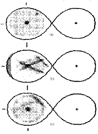
Figure 3.13: Suppression of arcs in the reconstructed image. (a) The original accretion disc image, with two Gaussian spots superimposed on a uniform background. (b) The image obtained using the uniform default map. (c) The image obtained using the default of full azimuthal smearing. Adapted from Horne (1985).

Choosing a non-uniform default map allows prior expectation of the likely disc intensity map to be included in the procedure. Baptista (2001) discusses some useful prescriptions for the default, listed in table 3.4.

The default $D_{j}$ usually takes the form of a weighted average of the intensities $I_{k}$ of the elements in the grid:

$$D_{j}=\frac{\sum_{k}\omega_{jk}I_{k}}{\sum_{k}\omega_{jk}},$$ (3.29)

where $\omega_{jk}$ is the user-defined weight function. It is ultimately via the weight function that a priori information about the disc is included in the reconstruction. The weight function is usually defined as a Gaussian point-spread function of width $\Delta$.

Table 3.4: Prescriptions for weight functions $\omega_{jk}$. $d_{jk}$ is the distance between pixels $j$ and $k$; $R_{j}$ and $R_{k}$ are the distances of pixels $j$ and $k$ from the origin, respectively; $\theta_{jk}$ is the azimuthal angle between pixels $j$ and $k$; and $s_{jk}=|R_{j}\theta_{j}-R_{k}\theta_{k}|$ is the arc length between pixels $j$ and $k$. 1–5 from Baptista (2001).

1)	Most uniform map	$\omega_{jk}=1$
2)	Smoothest map	$\omega_{jk}=\exp\left(-\frac{d^{2}_{jk}}{2\Delta^{2}}\right)$
3)	Most axi-symmetric map	$\omega_{jk}=\exp\left[-\frac{(R_{j}-R_{k})^{2}}{2\Delta^{2}_{R}}\right]$
	(full azimuthal smearing)
4)	Limited azimuthal smearing	$\omega_{jk}=\exp\left[-\frac{1}{2}\left\{\left(\frac{R_{j}-R_{k}}{\Delta_{R}}\right)^{2}+\left(\frac{\theta_{jk}}{\Delta_{\theta}}\right)^{2}\right\}\right]$
	(constant angle $\theta$)
5)	Limited azimuthal smearing	$\omega_{jk}=\exp\left[-\frac{1}{2}\left\{\left(\frac{R_{j}-R_{k}}{\Delta_{R}}\right)^{2}+\left(\frac{s_{jk}}{\Delta_{s}}\right)^{2}\right\}\right]$
	(constant arc length $s$)
6)	Limited azimuthal smearing	$\omega_{jk}=\exp\left[-\frac{1}{2}\left(\frac{\theta_{jk}}{\Delta_{\theta}}\right)^{2}\right]$
	(for disc rim)

One would expect the discs in CVs to be roughly axi-symmetric since the material in the disc is, to a first approximation at least, in Keplerian orbits. By using the prescriptions for the default map given in table 3.4 this expectation can be included in the default map. The effect of this is that the entropy becomes insensitive to structure on scales larger than $\Delta$. Structure on small scales will be suppressed by the entropy, whereas large-scale structure will be freely determined by the data. This can be seen from study of the weight functions given in table 3.4. If the numerator is much smaller than $\Delta$ then the weight will be large; if the numerator is larger than the denominator $\Delta$ then the weight will be small. Figure 3.13 shows the effect of the default of full azimuthal smearing (see table 3.4). Some remnants of the spurious arcs remain, but they are greatly reduced in amplitude.

The default of full azimuthal smearing can result in distorted reconstructions of discrete structures in the disc. For instance, the bright spot is often smeared out into a ring of the same radial distance from the white dwarf as the bright spot. In order to limit this distortion, a default map of limited azimuthal smearing can be used. Two methods of achieving this have been proposed: a weight function of constant angles (Rutten et al., 1993) and a weight function of constant arc length (Baptista et al., 1996). The default of constant angles gives better resolution in the inner parts of the disc, whereas the default of constant arc length gives better resolution in the outer parts of the disc (see Baptista (2001) and figure 3.14). For the data presented in this thesis, it was found that the difference between the maps reconstructed using the defaults of constant angles and constant arc length was negligible, and therefore the default used throughout this thesis was that of limited azimuthal smearing (constant angles).

A different default map was used for the disc rim to reflect its constant radial distance from the centre of the grid and to allow the rim intensity to be independent of the intensity distribution of the $(x,y)$ grid. In order to fulfil this latter criterion, the weight of each pixel in the disc rim with respect to each pixel in the $(x,y)$ grid was zero, and vice versa. The default chosen for the disc rim was number 6 in table 3.4, with $\Delta_{\theta}({\rm rim})=\Delta_{\theta}({\rm disc})$.

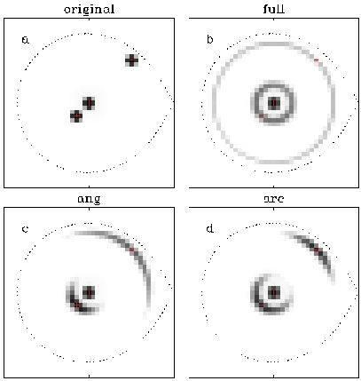
Figure 3.14: The effect of different weight functions on the default map. (a) shows the original map, with three Gaussian spots. The remaining panels show the default maps (note: not the reconstructed maps) produced from the map illustrated in panel (a) by applying the weight functions (see table 3.4) of (b) full azimuthal smearing, (c) constant angle $\theta$ and (d) constant arc length $s$. From Baptista et al. (1996).

The orbital hump

The first method I attempted to use to correct for the orbital hump followed Baptista et al. (2000), who fitted a spline function to phases outside eclipse, divided the light curve by the fitted spline and scaled the result to the value of the spline function at phase zero, in order to scale the light curve back to the original flux level (see also Horne, 1985). This technique worked well on the light curve of IP Peg in outburst to which Baptista et al. (2000) applied it, but it is not suitable for the light curves of quiescent dwarf novæ which are the subject of this thesis. This is because by fitting and dividing by a spline function we assume that all parts of the accretion disc contribute equally to the anisotropic flux (the orbital hump). This is not the case: the bright spot produces anisotropic radiation, whereas the white dwarf and accretion disc do not (Horne, 1985; Bobinger et al., 1997).

The method I eventually employed in order to model the orbital hump was to introduce a disc rim (e.g. Bobinger et al., 1997). This rim is assumed to be of negligible height (so that I still assume a flat disc) and is divided into $m$ segments. The visibility function $V(i,\phi)$ for the rim is given by

$$V(i,\phi)=\left\{\begin{array}[]{ll}0&\mbox{if eclipsed}\\ 0&\mbox{if $\sin(\theta+\phi)<0$}\\ \sin^{2}(\theta+\phi)&\mbox{otherwise}\end{array}\right.,$$ (3.30)

where $\theta$ is the angle between the position on the disc rim and the positive x-axis, measured clockwise. The intensity of each element of the disc rim was fitted along with the intensity of each of the Cartesian grid elements, and was found to model the orbital hump very effectively. The number of elements used to model the disc rim was 50 for all the reconstructions in this thesis. This number was chosen to be high enough to effectively reproduce the orbital hump and low enough so that the orbital modulation was reasonably smooth.

The contribution of the secondary star

The flux from the secondary star can have a detrimental effect on the quality of the reconstructed map. This is because the relative eclipse depth is anti-correlated with the eclipse width; any uneclipsed light breaks this anti-correlation. The additional light is placed by the maximum entropy reconstruction in the parts of the map which are constrained the least by the eclipse data, such as the parts of the accretion disc farthest from the red dwarf (the ‘back’ of the disc). This is discussed in detail by Rutten et al. (1992, 1994); Baptista et al. (1995, 1996). These authors find that the contribution from the secondary can be estimated by maximum entropy methods. First, the light curve can be offset by varying amounts and fitted using the usual eclipse mapping procedure. The offset which allows the largest entropy to be achieved is then the uneclipsed light. Second, and equivalently, an additional ‘virtual pixel’ can be introduced into the grid. If the visibility function for this pixel is unity at all phases, and its weight (refer to equation 3.29) with respect to all the other pixels is zero, and unity with respect to itself, then from the definition of the $\chi^{2}$ statistic (equation 3.6) the contribution of this pixel to the entropy measure is zero, and the iterative procedure to maximise the entropy proceeds as usual. The only effect of this virtual pixel on the intensities of all other pixels in the reconstruction is an offset, the magnitude of which is determined by the maximum entropy procedure itself. This method of determining the contribution from the secondary star fails for highly asymmetric accretion discs, as noted by Baptista et al. (1996). The spurious structure introduced in the reconstructed map by the uneclipsed component mixes with the asymmetric (bright spot) emission, forming a more azimuthally symmetric structure in the disc. Due to the choice of an azimuthally symmetric default map, this has the effect of increasing the entropy of the reconstructed map. The map with the largest entropy value is therefore not that with the correct offset due to the presence of uneclipsed light. This problem is particularly severe in the case of the faint, short-period dwarf novæ such as XZ Eri and DV UMa studied in this thesis, as the disc is effectively invisible in these objects, meaning that almost all of the emission originates from the bright spot region: the disc emission is highly asymmetric.

I have therefore subtracted the contribution to the total light from the secondary star from the light curve prior to fitting. In the cases of XZ Eri and DV UMa, the secondary contribution was determined from the lfit procedure. For all other objects, the contribution of the secondary star was first estimated from the mid-eclipse flux level, and fine-tuned by computing a series of eclipse maps with different offset values and selecting the map with the least spurious structure. These offsets are given in table  3.5.

The iterative procedure

The memsys code iteratively adjusts the intensities of each element $h_{j}$. The procedure begins with a uniform intensity distribution, in which each element has an intensity equal to the maximum value of the light curve divided by the total number of elements. This obviously gives a poor fit to the data. The code then iterates until the desired $\chi^{2}_{\rm R}$, known as $\chi^{2}_{\rm R,aim}$, is achieved, subsequent iterations serving to maximise the entropy while keeping $\chi^{2}_{\rm R}$ fixed. The exit criterion, which when satisfied signals that the final solution has been reached, is $TEST<10^{-3}$, where

$$TEST=\frac{1}{2}\left|\frac{\Delta\chi^{2}_{\rm R}}{|\Delta\chi^{2}_{\rm R}|}-\frac{\Delta S}{|\Delta S|}\right|,$$ (3.31)

provided that $|\chi^{2}_{\rm R}-\chi^{2}_{\rm R,aim}|<1$ and that the entropy during the last five iterations has not decreased by more than 0.5 per cent. When the entropy has been maximised, $TEST$ should be zero, since in this case both $\Delta\chi^{2}_{\rm R}$ and $\Delta S$ will necessarily be small. This definition of $TEST$ is equivalent to that used internally by memsys: $TEST=1-\cos\theta$, where $\theta$ is the angle between the gradients of entropy $S$ and $\chi^{2}_{\rm R}$. The reconstructed images are those that are closest to the default map from those that are consistent with the data to $\chi^{2}_{\rm R,aim}$.

The choice of $\chi^{2}_{\rm R,aim}$ affects the properties of the reconstructed map. If too large a value is chosen, the map will not be well-constrained by the data (i.e. entropy will dominate), and the features present will be smeared out by the effects of the default map adopted. On the other hand, if too small a value of $\chi^{2}_{\rm R,aim}$ is used, then the reconstructed map will be noisy, with a characteristic ‘grainy’ texture, the result of trying to fit noise in the data. Note that the optimum value $\chi^{2}_{\rm R,aim}$ is usually greater than unity due to the presence of flickering in the light curve resulting in the scatter of the data points being greater than that implied by the errors on the data points.

To perform a maximum entropy reconstruction of the accretion disc, the program was first run with $\chi^{2}_{\rm R,aim}=1$. In almost all cases this $\chi^{2}_{\rm R,aim}$ was never achieved, so the program was re-started with a value for $\chi^{2}_{\rm R,aim}$ adopted that was reached in the previous attempt. The reconstructed image was visually inspected, the value of $\chi^{2}_{\rm R,aim}$ adjusted and the code re-run until the resulting intensity map was judged to be ‘non-grainy’ and the spurious arcs were minimised.

Testing of the eclipse mapping code

The eclipse mapping code was tested using the data for XZ Eri and DV UMa described in table 2.1 and chapter 5. The positions of the white dwarf and bright spot and the absence of a significantly luminous accretion disc formed the testing criteria. The XZ Eri and DV UMa data were used instead of creating fake light curves due to their high quality (especially for XZ Eri) and the fact that the system parameters were determined to a high degree of accuracy from my previous work using lfit (see § 5.3.2). The results of the eclipse mapping experiments are presented and discussed in subsequent chapters. For ease of reference, the parameters used in each reconstruction are given in table 3.5 below.

Table 3.5: The parameters used in the maximum entropy reconstructions of the disc intensities. For each reconstruction, the default map is number 4 with $\Delta_{\theta}=0.7$ radians and $\Delta_{R}=0.01a$ (see table 3.4). The size of the grid in each case is $0.6a\times 0.6a$. The format of the quoted grid dimensions is x tiles $\times$ y tiles $+$ disc rim tiles. The tiles in the $x,y$ grid are subdivided as described in § 3.7.2. Some light curves were rebinned by the factor shown (using a weighted mean) in order to reduce flickering.

Object	Cycle	Filter	$\chi^{2}_{\rm R,aim}$	Grid	Sub-	Iterations	Phase	Secondary	Binning	Radius of
				dimensions	divisions		range	(mJy)	factor	disc rim ($a$)
XZ Eri	all	u′	1.15	$59\times 59+50$	2	33	all	0.0020	–	0.3
	all	g′	1.4	$59\times 59+50$	2	32	all	0.0029	–	0.3
	all	r′	2.5	$59\times 59+50$	2	36	all	0.0064	–	0.3
DV UMa	all	u′	1.4	$71\times 71+50$	6	60	$-0.06$ to $0.13$	0.0027	–	0.31805
	all	g′	1.3	$71\times 71+50$	6	61	$-0.06$ to $0.13$	0.00531	–	0.31805
	all	i′	7.0	$71\times 71+50$	6	87	$-0.06$ to $0.13$	0.0680	–	0.31805
HT Cas	2002 data	u′	2.8	$75\times 75+50$	7	28	$-0.09$ to $0.09$	0.15	3	0.28
	2002 data	g′	24	$75\times 75+50$	7	29	$-0.09$ to $0.09$	0.09	3	0.28
	2002 data	i′	7	$75\times 75+50$	7	31	$-0.09$ to $0.09$	0.32	0	0.28
HT Cas	2003 data	u′	1.4	$75\times 75+50$	7	71	$-0.09$ to $0.09$	0.24	3	0.26
	2003 data	g′	15	$75\times 75+50$	7	74	$-0.09$ to $0.09$	0.14	3	0.26
	2003 data	i′	6	$75\times 75+50$	7	134	$-0.09$ to $0.09$	0.42	3	0.26
OU Vir	2002 5 18	u′	1	$70\times 70+50$	2	200	$-0.06$ to $0.1$	0.06	–	0.2315
	2002 5 18	g′	4.5	$70\times 70+50$	2	30	$-0.06$ to $0.1$	0.06	–	0.2315
	2002 5 18	r′	2.5	$70\times 70+50$	2	29	$-0.06$ to $0.1$	0.11	–	0.2315
OU Vir	2003 5 22	u′	1.5	$70\times 70+50$	2	28	$-0.06$ to $0.1$	0.04	–	0.2315
	2003 5 22	g′	9	$70\times 70+50$	2	54	$-0.06$ to $0.1$	0.024	–	0.2315
	2003 5 22	i′	3.0	$70\times 70+50$	2	26	$-0.06$ to $0.1$	0.09	–	0.2315
IR Com	all	u′	15	$65\times 65+50$	5	71	$-0.06$ to $0.1$	0.27	2	0.3
	all	g′	250	$65\times 65+50$	5	73	$-0.06$ to $0.1$	0.12	2	0.3
	all	i′	120	$65\times 65+50$	5	71	$-0.06$ to $0.1$	0.35	2	0.3
GY Cnc	all	u′	8	$74\times 74+50$	9	49	all	0.35	–	0.3
	all	g′	60	$74\times 74+50$	9	51	all	0.37	–	0.3
	2003 5 23	i′	11	$74\times 74+50$	9	53	all	2.1	–	0.3
	2003 5 19	z′	4.0	$74\times 74+50$	9	56	all	2.2	–	0.3

Chapter 4 OU Vir

The contents of this chapter have been published in the Monthly Notices of the Royal Astronomical Society, 347, 1173 and 354, 1279 as ULTRACAM photometry of the eclipsing cataclysmic variable OU Vir by Feline, Dhillon, Marsh, Stevenson, Watson, & Brinkworth (2004b, c). The exceptions to this are the eclipse mapping results presented in § 4.5, and the observations of 2003 May 18, which were overlooked for publication due to an error in the hand-written observing logs. The data were analysed using the derivative technique only, and not the lfit method, as the significant night-to-night and short-term (flickering) variability meant that the modelling approach of the latter technique was found to be unsuitable in this case. The reduction and analysis of the data are all my own, as is the text below. Dr. Vik Dhillon supervised all work presented here.

OU Vir is a faint (V$\sim 18$ mag; Mason et al., 2002) eclipsing CV with a period of 1.75 hr which has been seen in outburst and probably superoutburst (Vanmunster et al., 2000), marking it as an SU UMa dwarf nova. Mason et al. (2002) presented time-resolved, multi-colour photometry and spectroscopy of OU Vir, concluding that the eclipse is of the bright spot and disc, but not the white dwarf.

The observations of OU Vir are summarised in table 2.1, and the data reduction procedure is detailed in § 2.3. The light curves of OU Vir are shown in figure 4.1. The data of 2002 May were obtained during the first night of commissioning of ultracam and hence were adversely affected by typical commissioning problems, chiefly excess noise in the u^′ band and limited time resolution due to the dead-time between exposures. The data taken in 2003 had no such problems.

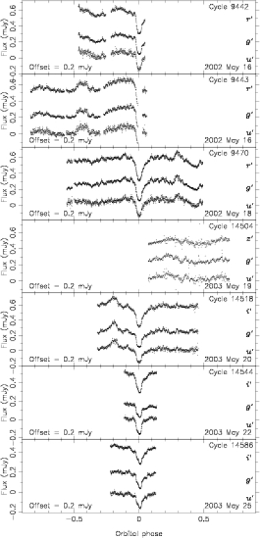
Figure 4.1: The light curve of OU Vir. The r^′, z^′ and i^′ data are offset vertically upwards and the u^′ data are offset vertically downwards.

4.1 Light curve morphology

Mason et al. (2002) found that for OU Vir out of eclipse and during quiescence, $V=18.08$ mag and $B-V=0.14$ mag, which corresponds to g${}^{\prime}\sim 0.2$ mJy (Smith et al., 2002). Vanmunster et al. (2000) quote an outburst amplitude of approximately 4 magnitudes (corresponding to a peak g^′ flux of $\sim 8.4$ mJy). OU Vir was observed at quiescence in both 2002 and 2003, as can be readily seen by inspection of figure 4.1. It is worth noting, however, that the 2003 observations took place about 18 days after a superoutburst of OU Vir was first reported, on 2003 May 2 (Kato, 2003). The light curves of 2002 May 16 (at phase $\sim-0.45$) and 18 (phase $\sim 0.3$) and 2003 May 20 (phase $\sim-0.2$) shown in figure 4.1 show a feature which strongly resembles a superhump, and suggests that the system may have recently undergone a superoutburst in 2002 as well as 2003.

Table 4.1: Mid-eclipse timings of OU Vir, accurate to $\pm 4\times 10^{-5}$ days.

Date	HJD
	u′	g′	r′	i′
2002 05 16	2452411.523977	2452411.523921	2452411.523892	–
2003 05 20	2452780.580157	2452780.580278	–	2452780.580217
2003 05 22	2452782.470534	2452782.470558	–	2452782.470509
2003 05 25	2452785.524083	2452785.524083	–	2452785.524255

Table 4.2: White dwarf contact phases, accurate to $\pm 0.0006$, and flux, accurate to $\pm 0.01$ mJy, of OU Vir.

Date	Band	$\phi_{\rm{w}1}$	$\phi_{\rm{w}2}$	$\phi_{\rm{w}3}$	$\phi_{\rm{w}4}$	$\phi_{\rm{wi}}$	$\phi_{\rm{we}}$	Flux (mJy)
2002 05 16	u′	$-0.024414$	$-0.017578$	$0.018555$	$0.025391$	$-0.020508$	$0.022461$	–
	g′	$-0.027344$	$-0.018555$	$0.016602$	$0.025391$	$-0.022461$	$0.021484$	–
	r′	$-0.028320$	$-0.013672$	$0.012695$	$0.027344$	$-0.020508$	$0.020508$	–
2003 05 20	u′	$-0.023438$	$-0.016602$	$0.018555$	$0.025491$	$-0.019531$	$0.022461$	–
	g′	$-0.025391$	$-0.017578$	$0.017578$	$0.024414$	$-0.021484$	$0.021484$	–
	i′	$-0.023438$	$-0.014648$	$0.016602$	$0.025391$	$-0.018555$	$0.021484$	–
2003 05 22	u′	$-0.024414$	$-0.016602$	$0.017578$	$0.025391$	$-0.020508$	$0.021484$	–
	g′	$-0.026367$	$-0.018555$	$0.016602$	$0.024414$	$-0.022461$	$0.020508$	–
	i′	$-0.021484$	$-0.018555$	$0.016602$	$0.020508$	$-0.019531$	$0.018555$	–
2003 05 25	u′	$-0.025391$	$-0.016602$	$0.014648$	$0.023438$	$-0.020508$	$0.019531$	$0.0537$
	g′	$-0.025391$	$-0.019531$	$0.016602$	$0.022461$	$-0.022461$	$0.019531$	$0.0519$
	i′	$-0.022461$	$-0.018555$	$0.017578$	$0.022461$	$-0.020508$	$0.020508$	$0.0146$

Table 4.3: Bright spot contact phases of OU Vir, accurate to $\pm 0.0006$. The weakness of the bright spot feature and the presence of flickering in the light curves meant that it was not possible to accurately determine the bright spot contact phases for all the light curves.

Date	Band	$\phi_{\rm{b}1}$	$\phi_{\rm{b}2}$	$\phi_{\rm{b}3}$	$\phi_{\rm{b}4}$	$\phi_{\rm{bi}}$	$\phi_{\rm{be}}$
2003 05 22	g′	$-0.002930$	$0.002930$	–	–	$0.000977$	–
2003 05 25	u′	$-0.007813$	0$.002930$	$0.060547$	$0.065430$	$-0.002930$	$0.062500$
	g′	$-0.007813$	$0.002930$	$0.058594$	$0.068359$	$-0.002930$	$0.062500$

4.2 Eclipse contact phases

The white dwarf eclipse contact phases (defined in § 3.2) given in tables 4.1 and 4.3 were determined using the techniques described in § 3.2. Once the white dwarf eclipse contact phases had been found, the white dwarf light curve was reconstructed (as discussed in § 3.2) and subtracted from the overall light curve, as illustrated in figure 4.2. The out-of-eclipse white dwarf fluxes thus found are given in table 4.3. The white dwarf flux can be used to determine its temperature and distance; see § 3.6. Once this has been done the bright spot eclipse contact phases (given in table 4.3) can be determined by a similar method (Wood et al., 1989a) and its light curve removed from that of the disc eclipse. If successful, this process can be used to determine the bright spot temperature. Unfortunately I was unsuccessful in my attempts to do this, probably because flickering hindered accurate determination of the bright spot flux and contact phases.

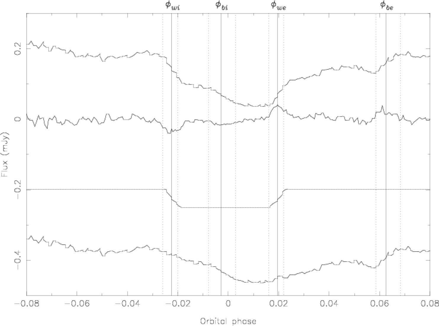
Figure 4.2: White dwarf deconvolution of the g^′ band light curve of OU Vir of 2003 May 25. Top to bottom: The data after smoothing by a median filter; the derivative after smoothing by a box car filter and subtraction of the spline fit to this, multiplied by a factor of 5 for clarity; the reconstructed white dwarf light curve, shifted downwards by 0.25 mJy; the original light curve minus the white dwarf light curve after smoothing by a median filter, shifted downwards by 0.5 mJy. The vertical lines show the contact phases of the white dwarf and bright spot eclipses (see § 3.2), the dotted lines corresponding to $\phi_{\rm{w}1}\ldots\phi_{\rm{w}4}$, $\phi_{\rm{b}1}\ldots\phi_{\rm{b}4}$ and the solid lines (labelled) to $\phi_{\rm{wi}}$, $\phi_{\rm{we}}$ and $\phi_{\rm{bi}}$, $\phi_{\rm{be}}$. The bright spot ingress and egress are plainly visible, quickly following the white dwarf ingress and egress respectively.

4.3 Orbital ephemeris

A linear least-squares fit to the times of mid-eclipse given in table 4.1 (calculated using the techniques described in § 3.2 and taking the midpoint of the white dwarf eclipse as the point of mid-eclipse) and those of Vanmunster et al. (2000, private communication) gives the following ephemeris:

$$\begin{array}[]{ccrcrl}\\ HJD&=&2451725.03283&+&0.072706113&E.\\ &&7&\pm&5&\end{array}$$

Errors of $\pm 4\times 10^{-5}$ days were used for the ultracam data, and errors of $\pm 7\times 10^{-4}$ days for the Vanmunster et al. (2000, private communication) data. This ephemeris was used to phase all of the data.

I do not present an $O-C$ (observed times of mid-eclipse minus times of mid-eclipse caluclated using an ephemeris) diagram as first, the mid-eclipse times reported by Vanmunster et al. (2000, private communication) were times predicted by their ephemeris for the cycle numbers they observed, and second, the time resolution of their data was too poor (between 30–160 seconds). Any $O-C$ diagram would therefore be meaningless.

4.4 System parameters

The derivation of the system parameters of OU Vir proceeds as discussed in § 3.2. Figure 4.3 shows the theoretical gas stream trajectory for $q=0.175$. As illustrated in figures 4.4 and 4.5, which show expanded views of the bright spot region, I constrain the light centre of the bright spot to be the point where the gas stream and outer edge of the disc intersect. The 2003 bright spot timings thus yield a mass ratio of $q=0.175\pm 0.025$ and an inclination of $i=79.2^{\circ}\pm 0.7^{\circ}$ for an eclipse phase width $\Delta\phi=0.0416\pm 0.0008$. The errors are determined by the rms variations in the measured contact phases.

Figures 4.4 and 4.5 show the eclipse constraints on the structure of the bright spot. I use these to determine upper limits on the angular size and the radial and vertical extent of the bright spot, with $\Delta\theta$, $\Delta R_{\rm{d}}$, $\Delta Z$ and $\Delta Z_{2}$ defined as in equations 3.3a–3.3d. The mean position and extent of the bright spot are given in table 4.4. From figures 4.4 and 4.5 I estimate visually that the gas stream passing through the light centre of the bright spot could just touch the phase arcs corresponding to $\phi_{\rm{b}1}$ and $\phi_{\rm{b}4}$ for a stream of circular cross-section with a radius $\varepsilon/a=0.0175\pm 0.0025$. The bright spot appears to be more extended azimuthally than radially, which can be understood by the shock front extending both up-disc and down-disc from the point of impact. The size of the stream is similar to that expected from theoretical studies (Lubow & Shu, 1975, 1976) and that obtained by studies of similar objects (Wood et al., 1986, 1989a), so the assumption that the stream passes through the light centre of the bright spot is reasonable.

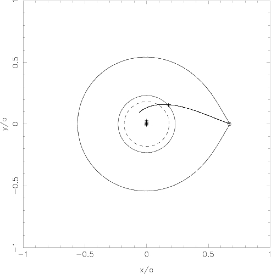
Figure 4.3: Trajectory of the gas stream from the secondary star for OU Vir, with $q=0.175$ and $i=79.2^{\circ}$. Top: The system with the primary Roche lobe, L₁ point and disc of radius $R_{\rm{d}}=0.2315a$ plotted. The positions of the white dwarf and bright spot light centres corresponding to the observed ingress and egress phases for $q$ and $i$ as above are also plotted. The circularisation radius (Verbunt & Rappaport, 1988, their equation 13) of $R_{\rm{circ}}=0.1820a$ is shown as a dashed circle. The stream passes through the bright spot points (note that the timings of 2003 May 22 are of the ingress only which prevents it from being plotted).

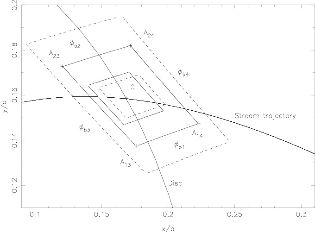
Figure 4.4: Horizontal structure of the bright spot of OU Vir for $q=0.175$, showing the region on the orbital plane within which the bright spot lies. The light centre LC is marked by a cross, surrounded by the inner solid box which corresponds to the rms variations in position. The phase arcs which correspond to the bright spot contact phases are shown as the outer solid box, with the rms variations in position shown as the two dashed boxes. As all the timings of $\phi_{\rm{b}2}$ and $\phi_{\rm{be}}$ are identical, the rms variations of $\phi_{\rm{b}1}$ and $\phi_{\rm{bi}}$, respectively, have been used instead. Intersections of the phase arcs $\phi_{{\rm b}j}$ and $\phi_{{\rm b}k}$ are marked $A_{jk}$, with crosses. The stream trajectory and disc of radius $R_{\rm{d}}=0.2315a$ are also plotted as solid curves.

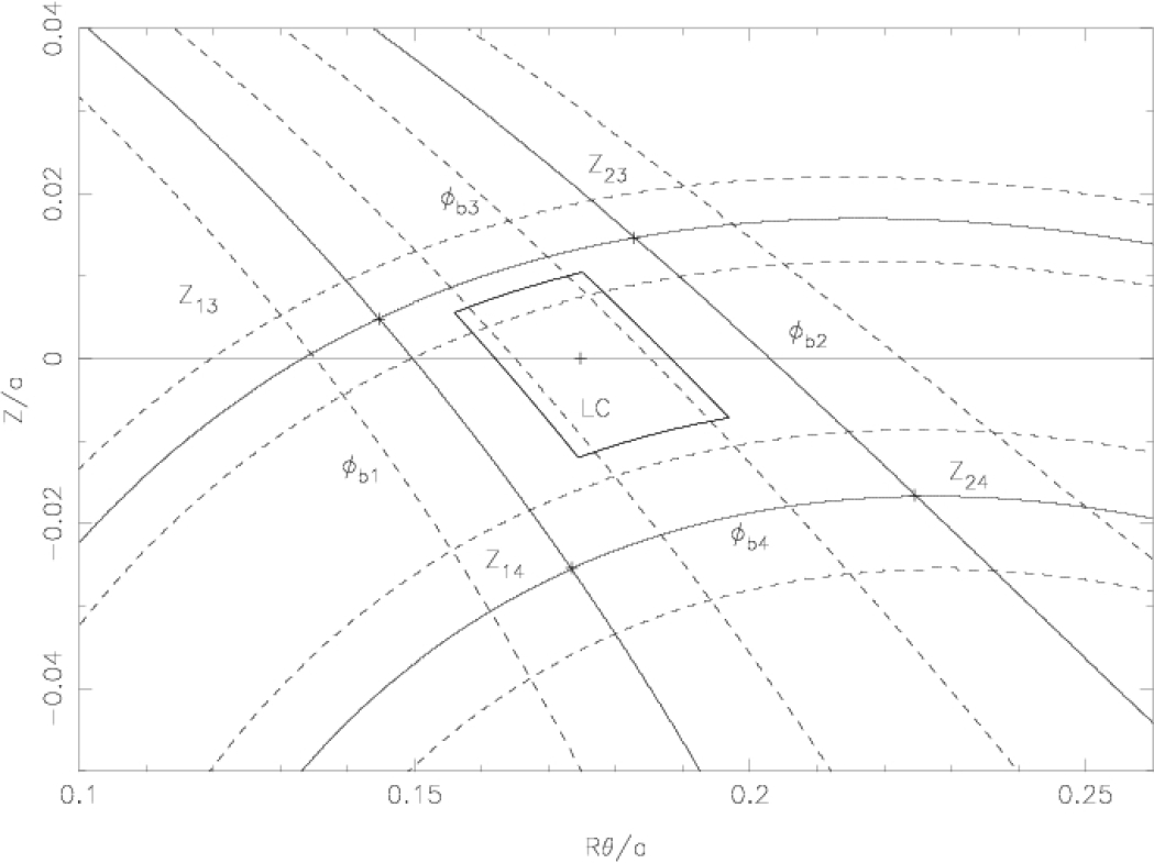
Figure 4.5: As figure 4.4, but showing the vertical structure of the bright spot. The phase arcs are projected onto a vertical cylinder of radius $0.2315a$ (equal to that of the disc), i.e. the x-axis is stepping around the edge of the disc. $\theta$ is in radians. The intersections of the phase arcs $\phi_{{\rm b}j}$ and $\phi_{{\rm b}k}$ are marked $Z_{jk}$, with crosses.

Figure 4.6 shows the eclipse constraints on the radius of the white dwarf. Using the mass ratio and orbital inclination derived earlier, I find that the white dwarf has a radius of $R_{1}=0.013\pm 0.004a$. An alternative possibility is that the sharp eclipse is caused by a bright inner disc region or boundary layer of radius $R_{\rm{belt}}=0.023\pm 0.010a$ surrounding the white dwarf like a belt. These errors are calculated using the rms variations in the measured contact phases. Another possibility is that the lower hemisphere of the white dwarf is obscured by an optically thick accretion disc, which would result in the white dwarf radius being $R_{1}\geq 0.013a$. This can be seen from inspection of figure 4.6 and considering that the phase arcs $\phi_{\rm w1}$ and $\phi_{\rm w4}$ in this case correspond to the lowest unobscured sections of the white dwarf. As discussed in § 3.2, for a symmetrical light distribution centred on the origin, as we would expect of a white dwarf, then the contact phases $\phi_{\rm{wi}}$ and $\phi_{\rm{we}}$ lie half-way through the white dwarf ingress and egress. Figure 4.6 illustrates that this is indeed the case, and so it is probable that the lower half of the white dwarf remains unobscured.

The determination of the absolute system parameters assumes that the eclipse is solely of a white dwarf. If the eclipse is actually of a belt and the white dwarf itself is not visible, then the white dwarf radius must be smaller than $R_{\rm{belt}}=0.023a$. If the white dwarf does contribute significantly to the eclipsed light, then we have the additional constraint that its radius must be $R_{1}\leq 0.013a$, so that the white dwarf mass given in table 4.5 is actually a lower limit. The only way to verify the assumption that the central light source is the white dwarf alone is to measure the semi-amplitude of the radial velocity curve of the secondary star, $K_{\rm{2}}$, and compare it to that predicted by the photometric model in table 4.5. One could also check if this assumption is true using a longer baseline of quiescent observations, as one might expect eclipse timings of an accretion belt to be much more variable than those of a white dwarf. I note, however, that the white dwarf mass given in table 4.5 is consistent with the mean white dwarf mass of $0.69\pm 0.13\;{\rm M}_{\odot}$ for CVs below the period gap (Smith & Dhillon, 1998). Also, as discussed in § 3.2, short-period dwarf novæ like OU Vir tend to accrete directly onto the white dwarf, whereas longer-period dwarf novæ usually have boundary layers. The system parameters of OU Vir, assuming that the central eclipsed object is indeed a white dwarf, are given in table 4.5.

The superhump period of OU Vir is $P_{\rm sh}=0.078\pm 0.002$ days (Vanmunster et al., 2000), which means that OU Vir lies $5\sigma$ off the superhump period excess–mass ratio relation of Patterson (1998, his equation 8), with the superhump period excess $\epsilon=(P_{\rm sh}-P_{\rm orb})/P_{\rm orb}\sim 0.073$. However, it does not lie on the superhump period excess-orbital period relation either, perhaps indicating that the current estimate of the superhump period $P_{\rm sh}$ is inaccurate.

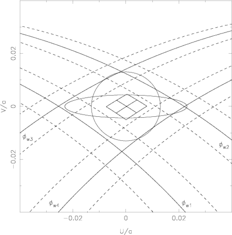
Figure 4.6: Projection of the white dwarf phase arcs of OU Vir onto the plane perpendicular to the line of sight. $U$ and $V$ are orthogonal co-ordinates perpendicular to the line of sight, $U$ being parallel to the binary plane. Solid curves correspond to the contact phases of the white dwarf, dotted curves to the rms variations of the phase arcs. The light centre is also plotted surrounded by the solid box corresponding to the rms variations in phase. The projection of the white dwarf and accretion belt centred on $U,V=0$ are shown for $R_{1}=0.013a$ and $R_{\rm{belt}}=0.023a$.

Table 4.4: Mean position and extent of the bright spot of OU Vir as defined by equations 3.3a–3.3c. $\Delta Z_{2}$ is calculated according to the definition used by Wood et al. (1986), for ease of comparison.

$\Delta R_{\rm{d}}/a$	0.0417
$\Delta\theta$	$15.17^{\circ}$
$\Delta Z/a$	0.0200
$\Delta Z_{2}/a$	0.0147
$R_{\rm{d}}/a$	0.2315
$\theta$	$43.24^{\circ}$

Table 4.5: System parameters of OU Vir. The secondary radius given is the volume radius of the secondary’s Roche lobe (Eggleton 1983), as defined by equation 1.4. Parameters left blank in the right-hand column are independent of the model used. The radial velocities quoted are estimated from the derived system parameters.

Parameter	Nauenberg (cold)	Nauenberg ($21\,700$ K)
Inclination $i$	$79.2^{\circ}\pm 0.7^{\circ}$
Mass ratio $q=M_{2}/M_{1}$	$0.175\pm 0.025$
White dwarf mass $M_{1}/{\rm M}_{\odot}$	$0.85\pm 0.20$	$0.90\pm 0.19$
Secondary mass $M_{2}/{\rm M}_{\odot}$	$0.15\pm 0.04$	$0.16\pm 0.04$
White dwarf radius $R_{1}/R_{\odot}$	$0.0095\pm 0.0030$	$0.0097\pm 0.0031$
Secondary radius $R_{2}/{\rm R}_{\odot}$	$0.177\pm 0.024$	$0.181\pm 0.024$
Separation $a/{\rm R}_{\odot}$	$0.73\pm 0.06$	$0.75\pm 0.05$
White dwarf radial velocity $K_{1}/\rm{km\,s^{-1}}$	$75\pm 12$	$76\pm 12$
Secondary radial velocity $K_{2}/\rm{km\,s^{-1}}$	$426\pm 6$	$434\pm 6$
Outer disc radius $R_{\rm{d}}/a$	$0.2315\pm 0.0150$
Distance $D/\rm{pc}$	$650\pm 210$
White dwarf temperature $T_{1}/\rm{K}$	$21\,700\pm 1200$

4.5 Eclipse mapping

The eclipse maps of OU Vir presented in figures 4.7–4.10 were produced using the parameters given in table 4.5 and derived in § 4.4. The data of 2002 May 18 and 2003 May 22 were chosen as the eclipses are complete and relatively uncontaminated by flickering. The data of different nights could not have been phase-folded since there were significant differences between them. As expected for such short-period systems, none of the reconstructed maps show evidence for disc emission. The reconstructed maps of 2002 May 18 show a white dwarf at the centre of the disc and a bright spot, which appears to be at a larger radius than that derived in the previous section (which used the 2003 data). I speculate that this is due to an enlarged disc radius because of the system being in decline from outburst. The feature near the central white dwarf is probably spurious, due to the intersection of two phase arcs at that point which intersect the white dwarf and bright spot. The reconstructed maps of 2003 May 22 also show the central white dwarf and the bright spot. The bright spot position (assuming that it is located at the intersection of the disc and the gas stream) for these data corresponds to a disc radius smaller than that of 2002 May 18, but still slightly greater than derived in § 4.4. This is possibly an effect of the entropy smearing out the intensity distribution during the reconstruction process, but is more likely indicative of the uncertainty in estimating the eclipse contact phases in § 4.4, and possibly a change in the radius of the accretion disc over the course of the 2003 observations.

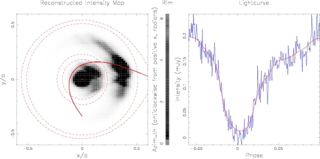
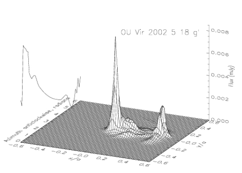
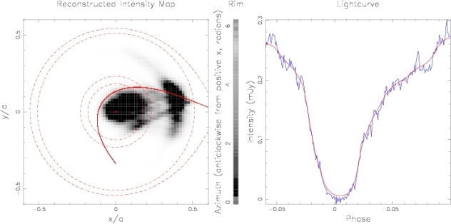
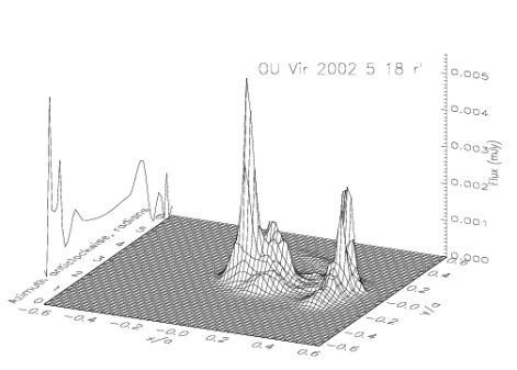
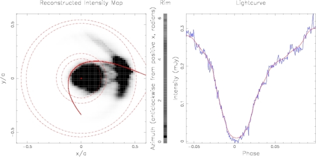
Figure 4.7: Top row. Left: a three-dimensional representation of the reconstructed accretion disc for the 2002 May 18 u^′ data of OU Vir. The white dwarf is at the origin, and the red dwarf at $(x,y)=(a,0)$. The rim intensity is shown on the edge of the grid. Centre: a two-dimensional view of the reconstructed accretion disc as before. The dot-dashed red lines are, from the centre out, the circularisation radius (Verbunt & Rappaport, 1988, their equation 13), the disc radius (the same radius as the rim), the tidal radius (Paczyński, 1977) and the primary star’s Roche lobe. The solid red line is the trajectory of the gas stream. The rim intensity is shown to the right. The scale is linear from zero to five per cent of the maximum, with areas with intensities greater than 5 per cent of the maximum shown in black. Dark regions are brighter. Right: The light curve (blue) with the fit (red) corresponding to the intensity distribution shown on the left overlaid. The middle and bottom rows are as the top, but for the g^′ and i^′ data, respectively. The system parameters adopted for the reconstruction are $q=0.175$, $i=79.2^{\circ}$ and $R_{\rm d}=0.2315a$ (the parameters given in table 4.5).

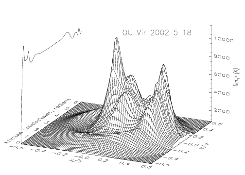
Figure 4.8: 3-dimensional plot of a blackbody fit to the reconstructed 2002 May 18 disc intensities of OU Vir shown in figure 4.7.

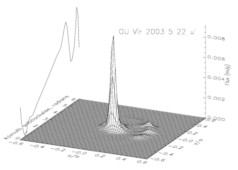
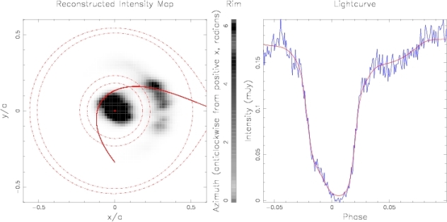
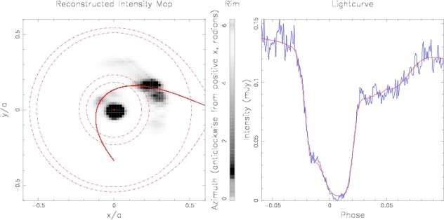
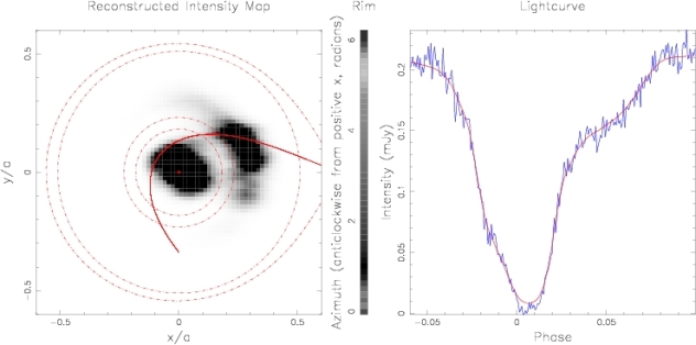
Figure 4.9: As figure 4.7, but for, from top, the u^′, g^′ and i^′ 2003 May 22 data of OU Vir. The system parameters adopted for the reconstruction are $q=0.175$, $i=79.2^{\circ}$ and $R_{\rm d}=0.2315a$ (the parameters given in table 4.5).

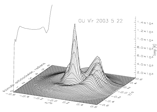
Figure 4.10: 3-dimensional plot of a blackbody fit to the reconstructed 2003 May 22 disc intensities of OU Vir shown in figure 4.9.

Chapter 5 XZ Eri and DV UMa

The contents of this chapter have been published in the Monthly Notices of the Royal Astronomical Society, 355, 1 as ULTRACAM photometry of the eclipsing cataclysmic variables XZ Eri and DV UMa by Feline, Dhillon, Marsh, & Brinkworth (2004a). The exceptions to this are the eclipse mapping results presented at the end of this chapter, in § 5.4. The system parameters were estimated using both the derivative and lfit techniques, as the light curves of both objects were largely free of flickering and were excellent candidates for model fitting. The reduction and analysis of the data are all my own, as is the text below. Dr. Vik Dhillon supervised all work presented here.

XZ Eri was first noted to be variable by Shapley & Hughes (1934). Until recently (Howell et al., 1991; Szkody & Howell, 1992), however, XZ Eri had been rather poorly studied. The presence of eclipses in the light curve of XZ Eri was discovered by Woudt & Warner (2001). More recently, Uemura et al. (2004) observed superhumps in the outburst light curve of XZ Eri, confirming its classification as an SU UMa star.

Previous observations of DV UMa are summarised by Nogami et al. (2001), who also present light curves obtained during the 1995 outburst and the 1997 superoutburst. Patterson et al. (2000) present superoutburst and quiescent photometry from which they derive the system parameters. Mukai et al. (1990) estimated the spectral type of the secondary star to be $\sim$M4.5 from spectroscopic observations.

In this chapter I present simultaneous three-colour, high-speed photometry of XZ Eri and DV UMa. I derive the system parameters via two separate methods—timings of the eclipse contact phases and fitting a parameterized model of the eclipse—and discuss the relative merits of each.

The observations of XZ Eri and DV UMa are summarised in table 2.1, and the data reduction procedure is detailed in § 2.3. The light curves of XZ Eri and DV UMa are shown in figures 5.1 and 5.2, respectively. The observations of XZ Eri began at high airmass (1.8)—this is evident in the improved quality of the second cycle, which was observed at lower airmass. Note also that the XZ Eri data of 2003 November 13 have significantly worse time-resolution than those of DV UMa, despite both objects being of similar magnitude. This is due to the higher brightness of the sky on 2003 November 13.

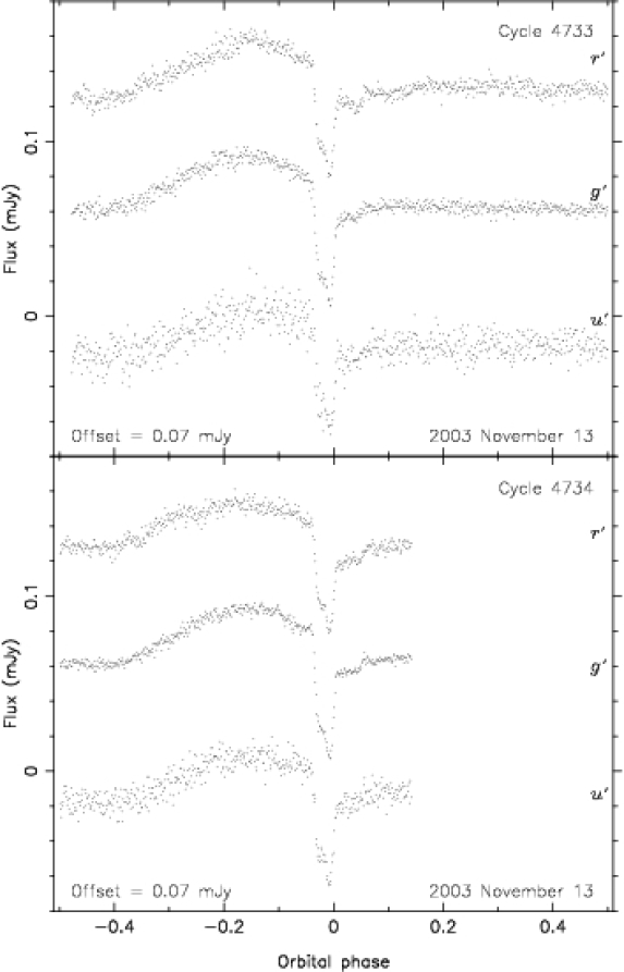
Figure 5.1: The light curve of XZ Eri. The data are contiguous. The r^′ data are offset vertically upwards and the u^′ data are offset vertically downwards.

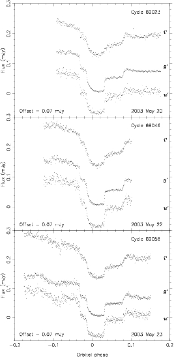
Figure 5.2: The light curve of DV UMa. The i^′ data are offset vertically upwards and the u^′ data are offset vertically downwards.

5.1 Light curve morphology

The light curve of XZ Eri shown in figure 5.1 is a classic example of an eclipsing dwarf nova. Between phase $-0.4$ and the start of eclipse, the orbital hump is clearly visible, with a brightening in g^′ flux of 0.025 mJy (0.5 mag). The light curve clearly shows separate eclipses of the white dwarf and bright spot (see figure 1.15) in all three colour bands.

During my observations XZ Eri had g${}^{\prime}\sim 19.5$ mag, falling to g${}^{\prime}\sim 21.5$ mag in mid-eclipse. Comparing this to the previous (quiescent) observations of Woudt & Warner (2001), who observed the system at $\rm{V}\sim 19.2$ mag, confirms that XZ Eri was in quiescence at the time of our observations.

The light curve of DV UMa is presented in figure 5.2. Although the phase coverage is less complete than for XZ Eri, the eclipse morphology is again typical of eclipsing short-period dwarf novæ. The white dwarf and bright spot ingress and egress are both clear and distinct. The orbital hump in DV UMa is much less pronounced than in XZ Eri.

Howell et al. (1988) quoted $\rm{V}\sim 19.2$ mag in quiescence for DV UMa. This compares to g${}^{\prime}\sim 19$ mag at the time of our observations, which fell to g${}^{\prime}\sim 22$ mag during eclipse. DV UMa was therefore in quiescence over the course of our observations.

5.2 Orbital ephemerides

The times of mid-eclipse $T_{\rm{mid}}$ given in table 5.1 were determined as described in § 3.2, taking the midpoint of the white dwarf eclipse as the the point of mid-eclipse.

To determine the orbital ephemeris of XZ Eri I used the one mid-eclipse time of Woudt & Warner (2001), the 25 eclipse timings of Uemura et al. (2004) and the six times of mid-eclipse given in table 5.1. I used errors of $\pm 5\times 10^{-4}$ days for the Woudt & Warner (2001) data, $\pm 1\times 10^{-4}$ days for the Uemura et al. (2004) timings and $\pm 4\times 10^{-5}$ days for the ULTRACAM data. A linear least-squares fit to these times gives:

$$\begin{array}[]{ccrcrl}\\ HJD&=&2452668.04099&+&0.061159491&E.\\ &&2&\pm&5&\end{array}$$

Table 5.1: Mid-eclipse timings $({\rm HJD}+2\,452\,000)$ of XZ Eri and DV UMa, accurate to $\pm 4\times 10^{-5}$ days.

XZ Eri cycle	u′	g′	r′
4733	957.508910	957.508789	957.508870
4734	957.570081	957.570000	957.570000
DV UMa cycle	u′	g′	i′
69023	780.469225	780.469225	780.469225
69046	782.443801	782.443829	782.443801
69058	783.474062	783.474040	783.474040

The orbital ephemeris of DV UMa was determined in a similar way using the 18 mid-eclipse timings of Nogami et al. (2001), the 12 timings of Howell et al. (1988), the 12 timings of Patterson et al. (2000) and the nine times of mid-eclipse given in table 5.1, with errors of $\pm 5\times 10^{-4}$ days assigned to the data of Nogami et al. (2001) and Howell et al. (1988), $\pm 1\times 10^{-4}$ days to the data of Patterson et al. (2000) and $\pm 4\times 10^{-5}$ days to the ULTRACAM data. A linear least-squares fit to these times gives:

$$\begin{array}[]{ccrcrl}\\ HJD&=&2446854.66157&+&0.0858526521&E.\\ &&9&\pm&14&\end{array}$$

These ephemerides were used to phase all of the data.

The $O-C$ diagrams for XZ Eri and DV UMa produced using the above ephemerides and times of mid-eclipse are shown in figures 5.3 and 5.4, respectively. Given the distribution of the data points for XZ Eri, it is not possible to determine if the system is undergoing period change or not. DV UMa, however, does show some evidence for period change, with a quadratic least-squares fit to the above times giving

$$\begin{array}[]{ccrcrlcll}\\ HJD&=&2446854.66283&+&0.085852592&E&+&6.2\times 10^{-13}&E^{2}.\\ &&14&\pm&5&&\pm&0.5&\end{array}$$

The $O-C$ diagram produced using the quadratic ephemeris for DV UMa is shown in figure 5.5. If accurate, the quadratic ephemeris implies a time scale for the period change of DV UMa of

$$P/\dot{P}=3.25\times 10^{7}\>{\rm yr}.$$

I believe that the period change of DV UMa is unlikely to be real in the sense that it represents the long-term evolutionary mean, and have therefore opted to use the linear ephemeris for DV UMa throughout this thesis. The reasons for this are two-fold. First, the eclipse timings of CVs often exhibit considerable ‘wander’ (e.g. IP Peg, Wood et al., 1989b), the cause of which is unclear. Second, the time resolution of the observations of Howell et al. (1988), which are the critical evidence for period change in the system, is comparable to the $O-C$ residuals for their observations shown in figure 5.4.

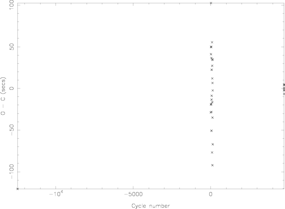
Figure 5.3: The $O-C$ diagram of XZ Eri produced using a linear ephemeris as described in the text.

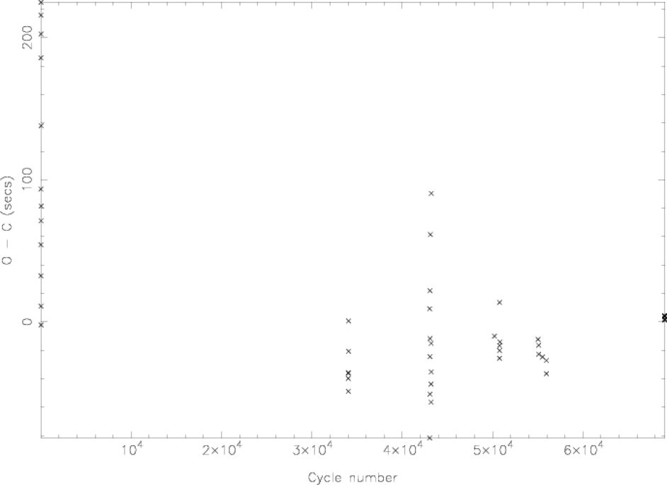
Figure 5.4: The $O-C$ diagram of DV UMa produced using a linear ephemeris as described in the text.

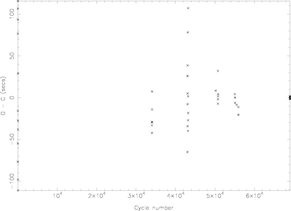
Figure 5.5: The $O-C$ diagram of DV UMa produced using a quadratic ephemeris as described in the text.

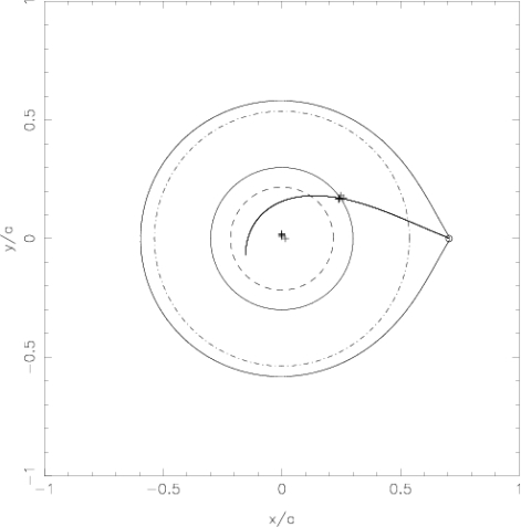
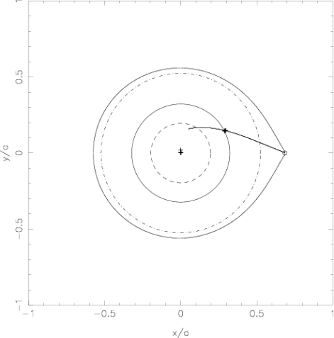
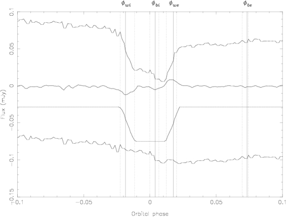
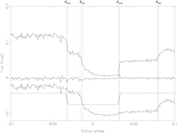
Figure 5.6: Top row: Trajectory of the gas stream from the secondary star for (left) XZ Eri ($q=0.117$, $i=80.3^{\circ}$, $R_{\rm{d}}/a=0.300$ and $R_{\rm{circ}}/a=0.217$) and (right) for DV UMa ($q=0.148$, $i=84.4^{\circ}$, $R_{\rm{d}}/a=0.322$ and $R_{\rm{circ}}/a=0.196$). The Roche lobe of the primary, the position of the inner Lagrangian point $\rm{L}_{1}$ and the disc of radius $R_{\rm{d}}$ are all plotted. The positions of the white dwarf and bright spot light centres corresponding to the observed ingress and egress phases are also plotted. The circularisation radius $R_{\rm{circ}}$ (Verbunt & Rappaport, 1988, their equation 13) is shown as a dashed circle, and the tidal radius (Paczyński, 1977) as a dot-dashed circle. Bottom row: White dwarf light curve deconvolution of (left) the g^′ band light curve of XZ Eri on 2003 November 13 (cycle 4733) and (right) the g^′ band light curve of DV UMa on 2003 May 23. Top to bottom: The data after smoothing by a median filter; the derivative after smoothing by a box-car filter and subtraction of a spline fit to this, multiplied by a factor of 1.5 for clarity; the reconstructed white dwarf light curve, shifted downwards by 0.075 mJy; the original light curve minus the white dwarf light curve after smoothing by a median filter, shifted downwards by 0.11 mJy. The vertical lines show the contact phases of the white dwarf and bright spot eclipses, the dotted lines corresponding to $\phi_{\rm{w}1},\ldots,\phi_{\rm{w}4}$, $\phi_{\rm{b}1},\ldots,\phi_{\rm{b}4}$ and the solid lines (labelled) to $\phi_{\rm{wi}}$, $\phi_{\rm{we}}$ and $\phi_{\rm{bi}}$, $\phi_{\rm{be}}$. The bright spot ingress and egress are plainly visible in the light curves of both objects, following the white dwarf ingress and egress, respectively.

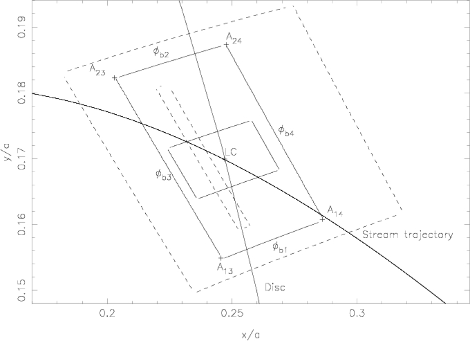
Figure 5.7: Horizontal structure of the bright spot of XZ Eri for $q=0.117$, showing the region on the orbital plane within which the bright spot lies. As figure 4.4, except that the disc radius is $R_{\rm{d}}=0.3a$.

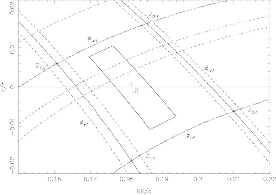
Figure 5.8: Vertical structure of the bright spot of XZ Eri for $q=0.117$. The phase arcs are projected onto a vertical cylinder of radius $0.3a$ (equal to that of the disc). Otherwise as figure 4.5.

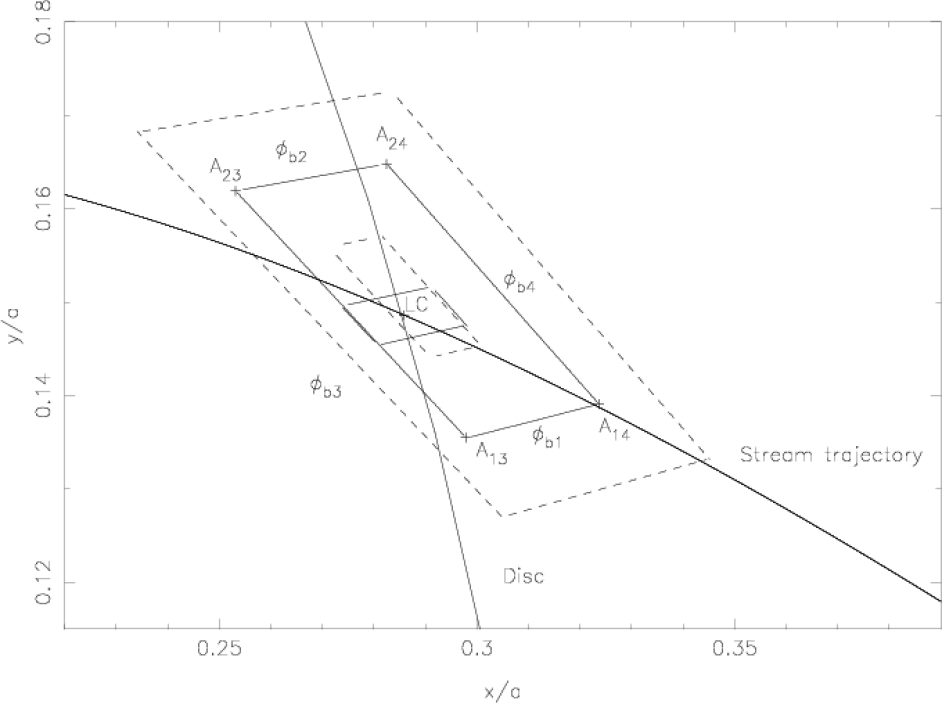
Figure 5.9: Horizontal structure of the bright spot of DV UMa for $q=0.148$, showing the region on the orbital plane within which the bright spot lies. As figure 4.4, except that the disc radius is $R_{\rm{d}}=0.322a$.

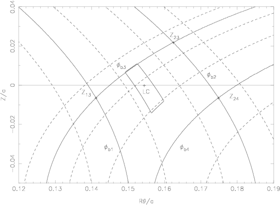
Figure 5.10: Vertical structure of the bright spot of DV UMa for $q=0.148$. The phase arcs are projected onto a vertical cylinder of radius $0.322a$ (equal to that of the disc). Otherwise as figure 4.5.

5.3 Light curve decomposition

5.3.1 The derivative method

The eclipse contact phases given in tables 5.2 and 5.3 were determined using the derivative of the light curve, as described in § 3.2. In the following analysis I have combined the timings of all three colour bands for each target in order to increase the accuracy of the results.

Using the techniques described in § 3.2, for the mean eclipse phase width of $\Delta\phi=0.0359\pm 0.0008$, the eclipse timings of XZ Eri (tables 5.2 and 5.3) yield the mass ratio, inclination and relative disc radius given in table 5.7. The results for DV UMa for the mean eclipse phase width of $\Delta\phi=0.0636\pm 0.0007$ are also given in table 5.7. The errors on these parameters are determined by the rms variations in the measured contact phases. I use the bright spot eclipse timings to determine upper limits on the angular size and the radial and vertical extent of the bright spots, defining $\Delta\theta$, $\Delta R_{\rm{d}}$, $\Delta Z$ and $\Delta Z_{2}$ as in equations 3.3a–3.3d. The mean position and extent of the bright spots thus derived are given in table 5.4. The eclipse constraints on the horizontal and vertical extent of the bright spots of XZ Eri and DV UMa are given in figures 5.7–5.10.

Using the mass ratio and orbital inclination given in table 5.7 and the eclipse constraints on the radius of the white dwarf (table 5.2), I find that the white dwarf in XZ Eri has a radius of $R_{1}/a=0.012\pm 0.002$. For DV UMa I obtain $R_{1}/a=0.0075\pm 0.0020$. I will continue under the assumption that the eclipsed central object is a bare white dwarf. This assumption and its consequences are discussed in more detail in § 3.2 and § 7.1.2.

The fluxes given in table 5.2 were fitted to the hydrogen-rich, $\log g=8$ white dwarf model atmospheres of Bergeron et al. (1995), as discussed in § 3.6. The colour indices quoted therein were converted to the SDSS system using the observed transformations of Smith et al. (2002). The white dwarf temperatures $T_{\rm{1}}$ thus calculated are given in table 5.7.

To determine the remaining system parameters of XZ Eri and DV UMa I used the Nauenberg mass–radius relation (equation 1.15) and approximated the secondary radius by its volume radius, as described in § 3.5. Because the Nauenberg mass-radius relation assumes a cold white dwarf, I have attempted to correct this to a temperature of $T_{\rm{1}}\sim 15\,000$ K for XZ Eri and to $T_{\rm{1}}\sim 20\,000$ K for DV UMa, the approximate temperatures given by the model atmosphere fit. The radius of the white dwarf at $10\,000$ K is about 5 per cent larger than for a cold ($0$ K) white dwarf (Koester & Schönberner, 1986). To correct from $10\,000$ K to the appropriate temperature, the white dwarf cooling curves of Wood (1995) for $M_{1}/{\rm M}_{\odot}=1.0$, the approximate masses given by the Nauenberg relation, were used. This gave total radial corrections of $6.0$ and $7.0$ per cent for XZ Eri and DV UMa, respectively.

Table 5.2: White dwarf contact phases, accurate to $\pm 0.0006$ (XZ Eri) and $\pm 0.0005$ (DV UMa), and out-of-eclipse white dwarf fluxes of XZ Eri and DV UMa. The errors on the fluxes are $\pm 0.001$ mJy.

Cycle	Band	$\phi_{\rm{w}1}$	$\phi_{\rm{w}2}$	$\phi_{\rm{w}3}$	$\phi_{\rm{w}4}$	$\phi_{\rm{wi}}$	$\phi_{\rm{we}}$	Flux (mJy)
XZ Eri
4733	u′	–0.020996	–0.015625	0.016113	0.022461	–0.018555	0.018555	0.0434
	g′	–0.022461	–0.011719	0.012207	0.020020	–0.018555	0.017578	0.0466
	r′	–0.022461	–0.013184	0.013184	0.020020	–0.019531	0.016113	0.0441
4734	u′	–0.018066	–0.014160	0.010742	0.020020	–0.017090	0.017578	0.0341
	g′	–0.022461	–0.013184	0.013672	0.021484	–0.019531	0.017578	0.0531
	r′	–0.022461	–0.013184	0.015137	0.020020	–0.017090	0.017578	0.0375
DV UMa
69023	u′	–0.033850	–0.030644	0.030276	0.033482	–0.031445	0.032680	0.0465
	g′	–0.033850	–0.030644	0.030276	0.033482	–0.031445	0.032680	0.0373
	i′	–0.033048	–0.029842	0.030276	0.033482	–0.030644	0.031879	0.0245
69046	u′	–0.032798	–0.030132	0.031210	0.033210	–0.031465	0.031877	0.0451
	g′	–0.033467	–0.030132	0.031210	0.033879	–0.032132	0.032543	0.0435
	i′	–0.032798	–0.030132	0.030544	0.033210	–0.030799	0.031877	0.0239
69058	u′	–0.032691	–0.030564	0.030612	0.032206	–0.030564	0.032206	0.0356
	g′	–0.033224	–0.030564	0.030612	0.032739	–0.031097	0.032206	0.0318
	i′	–0.033755	–0.030564	0.031142	0.033270	–0.032161	0.032739	0.0312

Table 5.3: Bright spot contact phases of XZ Eri and DV UMa, accurate to $\pm 0.0006$ (XZ Eri) and $\pm 0.0005$ (DV UMa).

Cycle	Band	$\phi_{\rm{b}1}$	$\phi_{\rm{b}2}$	$\phi_{\rm{b}3}$	$\phi_{\rm{b}4}$	$\phi_{\rm{bi}}$	$\phi_{\rm{be}}$
XZ Eri
4733	u′	–0.000977	0.006836	0.064941	0.067871	0.002930	0.066406
	g′	0.000000	0.006836	0.069336	0.074219	0.003906	0.073242
	r′	–0.000977	0.006836	0.069336	0.073242	0.001465	0.070313
4734	u′	–0.000977	0.006836	0.063965	0.081055	0.002930	0.070801
	g′	–0.000977	0.006836	0.065430	0.070801	0.001465	0.067871
	r′	0.000488	0.005859	0.065430	0.069336	0.002930	0.067871
DV UMa
69023	u′	–0.018620	–0.009803	0.079171	0.083179	–0.013811	0.082378
	g′	–0.016215	–0.011406	0.079171	0.083179	–0.013811	0.080775
	i′	–0.017017	–0.009001	0.078370	0.085584	–0.013009	0.079973
69046	u′	–0.016797	–0.012129	0.079884	0.085885	–0.014131	0.080553
	g′	–0.018130	–0.010129	0.079884	0.084552	–0.014131	0.081886
	i′	–0.022131	–0.006127	0.081220	0.083219	–0.014797	0.081886
69058	u′	–0.015671	–0.009819	0.079019	0.080613	–0.014074	0.079550
	g′	–0.015671	–0.010883	0.079019	0.081680	–0.013541	0.079550
	i′	–0.014604	–0.010883	0.077955	0.083274	–0.013010	0.078486

5.3.2 A parameterized model of the eclipse

The system parameters of XZ Eri and DV UMa were also determined by fitting the phase-folded light curves using a parameterized model of the eclipse. The lfit code, developed by Horne et al. (1994) and described in detail in § 3.3, was used.

The data were not good enough to determine the limb-darkening coefficient $U_{\rm{1}}$ accurately, so this was held at a typical value of 0.5 for each fit. The disc parameter for DV UMa was held fixed at $b=1.0$ as it was too faint to be well constrained.

The procedure discussed in § 3.3 failed to find the likely error for the disc exponent $b$ of the u^′ band of XZ Eri, as the disc flux is small in this case and the light curve noisy, so perturbation of the parameter made virtually no difference to the $\chi^{2}$ of the fit.

The results of the model fitting are given in tables 5.5 and 5.6, and are shown in figure 5.11. Each passband was fitted independently, as there were found to be significant differences between many of the optimum parameters for each band. This is to be expected for parameters such as the bright spot scale $SB$, where one would anticipate that the cooler regions are more extended than the hotter ones (as seen for DV UMa). We would, of course, expect the mass ratio to remain constant in all three passbands for each object, which it indeed does.

The results of a white dwarf model atmosphere fit (Bergeron et al., 1995) to the fluxes fit by the model in each passband are given in table 5.7. I have used the white dwarf cooling curves of Wood (1995) for $M_{1}/{\rm M}_{\odot}=0.75$ (interpolating between 0.7 and 0.8) and $M_{1}/{\rm M}_{\odot}=1.0$, the approximate masses found using the Nauenberg relation for XZ Eri and DV UMa, to give radial corrections of 7.6 and 7.0 per cent, respectively. These were used to determine the absolute system parameters given in table 5.7.

I note that the higher signal-to-noise light curves of the i^′, r^′ and g^′ bands have $\chi^{2}/\nu\gg 1$ (see tables 5.5 and 5.6). This is because these data are dominated by flickering, not photon noise, unlike the u^′ data. If we had enough cycles to completely remove the effects of flickering we would expect, for an accurate model, to achieve $\chi^{2}/\nu=1$.

The quality of the light curve fits (figure 5.11 and tables 5.5 and 5.6) are generally excellent. Apart from longer-term variations not allowed for by the model (for example, an overall brightening of the accretion disc), the only feature not satisfactorily reproduced is the bright spot egress of DV UMa. I suspect that this is due to the presence of ellipsoidal variations of the secondary star, which has the greatest contribution in this filter. Since the amplitude of the ellipsoidal modulation is at a minimum at phase zero, this will tend to enhance the amplitude of the orbital hump and shift the peak of the orbital hump towards the peak of the ellipsoidal modulation, at phase $-0.5$. In the case of the i^′ data of DV UMa shown in figure 5.11 the result of the algorithm trying to fit the increased flux at phases $\lesssim-0.1$ is to worsen the fit to the part of the orbital hump immediately following the egress of the bright spot. The contribution of the (M4.5; Mukai et al., 1990) secondary star in the i^′ band of DV UMa is comparable to that of the (M5.4; Marsh, 1990) secondary star of HT Cas (see also chapter 6). Due to the reason outlined above, and since not all of the orbital cycle of DV UMa was observed, the parameters that are constrained by the orbital hump are rather more uncertain for DV UMa than they are for XZ Eri. This may introduce some systematic errors into the estimation of the bright spot orientation $\theta_{\rm{B}}$, the isotropic flux fraction of the bright spot $f_{\rm iso}$ and the bright spot flux.

Table 5.4: Mean position and extent of the bright spots of XZ Eri and DV UMa, as defined in § 3.2.

	XZ Eri	DV UMa
$\Delta R_{\rm{d}}/a$	0.0378	0.0258
$\Delta\theta$	$8.73^{\circ}$	$7.57^{\circ}$
$\Delta Z/a$	0.0174	0.0399
$\Delta Z_{2}/a$	0.0161	0.0217
$R_{\rm{d}}/a$	0.300	0.322
$\theta$	$34.53^{\circ}$	$27.47^{\circ}$

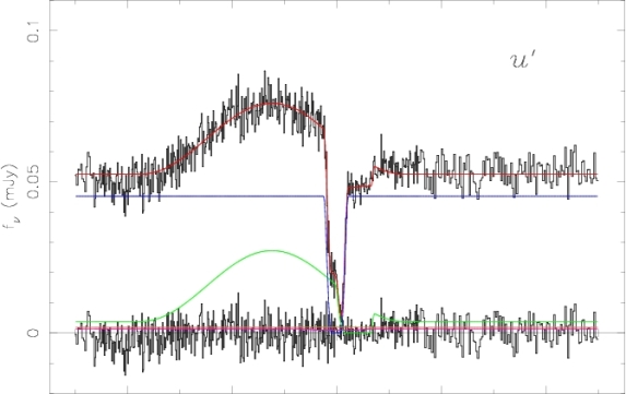
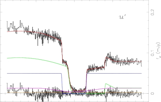
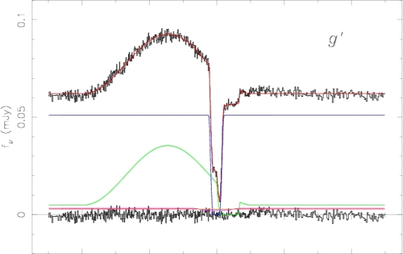
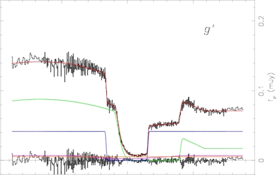
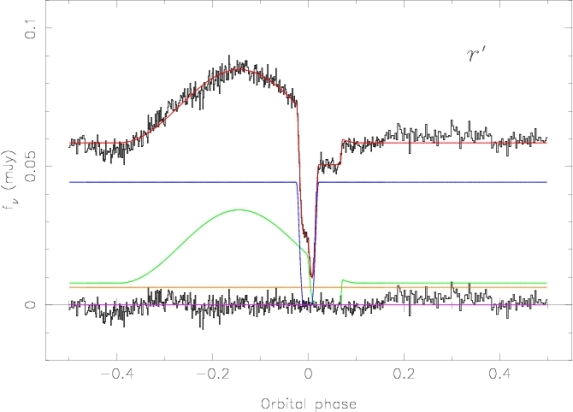
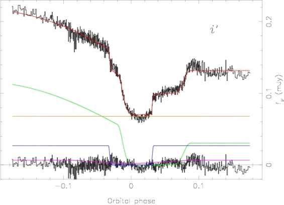
Figure 5.11: Left: the phase-folded u^′, g^′ and r^′ light curves of XZ Eri, fitted separately using the model described in Section 5.3.2. Right: the phase-folded u^′, g^′ and i^′ light curves of DV UMa. The data (black) are shown with the fit (red) overlaid and the residuals plotted below (black). Below are the separate light curves of the white dwarf (blue), bright spot (green), accretion disc (purple) and the secondary star (orange). Note that the disc in both objects is very faint, as is the secondary (except for the i^′ band of DV UMa). The differing phase coverage of each night’s observations of DV UMa accounts for the uneven appearance of the data.

Table 5.5: Parameters of XZ Eri fitted using a modified version of the lfit model of Horne et al. (1994) described in § 3.3. The fluxes of each component are also shown. XZ Eri has been fitted by phase-folding the two eclipses and binning by two data points. Note that the orbital inclination $i$ is not a fit parameter but is calculated using $q$ and $\Delta\phi$.

Parameter	XZ Eri
	u′	g′	r′
Inclination $i$	$80.4^{\circ}\pm 0.8^{\circ}$	$80.1^{\circ}\pm 0.1^{\circ}$	$80.4^{\circ}\pm 0.2^{\circ}$
Mass ratio $q$	$0.11\pm 0.02$	$0.116\pm 0.003$	$0.107\pm 0.002$
Eclipse phase	$0.0342$	$0.03362$	$0.0333$
width $\Delta\phi$	$\pm 0.0007$	$\pm 0.00021$	$\pm 0.0003$
Outer disc
radius $R_{\rm{d}}/a$	$0.307\pm 0.011$	$0.295\pm 0.003$	$0.316\pm 0.005$
White dwarf
limb	0.5	0.5	0.5
darkening $U_{\rm{1}}$
White dwarf
radius $R_{1}/a$	$0.019\pm 0.002$	$0.0175\pm 0.0006$	$0.0195\pm 0.0010$
Bright spot
scale $SB/a$	$0.014\pm 0.010$	$0.013\pm 0.002$	$0.0147\pm 0.0008$
Bright spot
orientation $\theta_{\rm{B}}$	$134.1^{\circ}\pm 1.0^{\circ}$	$141.9^{\circ}\pm 0.3^{\circ}$	$141.4^{\circ}\pm 0.3^{\circ}$
Isotropic flux
fraction $f_{\rm iso}$	$0.14\pm 0.03$	$0.140\pm 0.008$	$0.2294\pm 0.0015$
Disc exponent $b$	0.74965	$0.4\pm 2.1$	$0.3\pm 0.3$
Phase offset $\phi_{0}$	$16\times 10^{-4}$	$16.3\times 10^{-4}$	$17.0\times 10^{-4}$
	$\pm 3\times 10^{-4}$	$\pm 0.8\times 10^{-4}$	$\pm 1.2\times 10^{-4}$
$\chi^{2}$ of fit	656	897	1554
Number of
datapoints $\nu$	611	611	611
Flux (mJy)
White dwarf	$0.0453\pm 0.0011$	$0.0510\pm 0.0004$	$0.0443\pm 0.0004$
Accretion disc	$0.001\pm 0.003$	$0.0033\pm 0.0009$	$0.0000\pm 0.0010$
Secondary	$0.0020\pm 0.0019$	$0.0029\pm 0.0006$	$0.0064\pm 0.0007$
Bright spot	$0.0273\pm 0.0005$	$0.03545\pm 0.00018$	$0.0343\pm 0.0002$

Table 5.6: Parameters of DV UMa fitted using lfit. DV UMa has been fitted by phase-folding all three eclipses and binning by two data points. Otherwise as table 5.5.

Parameter	DV UMa
	u′	g′	i′
Inclination $i$	$83.8^{\circ}\pm 0.2^{\circ}$	$84.3^{\circ}\pm 0.1^{\circ}$	$84.3^{\circ}\pm 0.1^{\circ}$
Mass ratio $q$	$0.159\pm 0.003$	$0.1488\pm 0.0011$	$0.153\pm 0.002$
Eclipse phase	$0.06346$	$0.06352$	$0.06307$
width $\Delta\phi$	$\pm 0.00017$	$\pm 0.00007$	$\pm 0.00015$
Outer disc
radius $R_{\rm{d}}/a$	$0.317\pm 0.004$	$0.32278\pm 0.00016$	$0.31272\pm 0.00017$
White dwarf
limb	0.5	0.5	0.5
darkening $U_{\rm{1}}$
White dwarf
radius $R_{1}/a$	$0.0091\pm 0.0016$	$0.0092\pm 0.0004$	$0.0082\pm 0.0014$
Bright spot
scale $SB/a$	$0.0150\pm 0.0010$	$0.0211\pm 0.0002$	$0.049\pm 0.003$
Bright spot
orientation $\theta_{\rm{B}}$	$142.0^{\circ}\pm 0.8^{\circ}$	$137.75^{\circ}\pm 0.09^{\circ}$	$169.4^{\circ}\pm 0.6^{\circ}$
Isotropic flux
fraction $f_{\rm iso}$	$0.157\pm 0.009$	$0.1989\pm 0.0019$	$0.262\pm 0.004$
Disc exponent $b$	1.	1.	1.
Phase offset $\phi_{0}$	$2.5\times 10^{-4}$	$5.48\times 10^{-4}$	$1.7\times 10^{-4}$
	$\pm 0.9\times 10^{-4}$	$\pm 0.10\times 10^{-4}$	$\pm 0.7\times 10^{-4}$
$\chi^{2}$ of fit	1059	6873	4332
Number of
datapoints $\nu$	636	636	636
Flux (mJy)
White dwarf	$0.0496\pm 0.0008$	$0.0415\pm 0.0002$	$0.0269\pm 0.0004$
Accretion disc	$0.0131\pm 0.0015$	$0.0069\pm 0.0004$	$0.0065\pm 0.0007$
Secondary	$0.0027\pm 0.0007$	$0.00531\pm 0.00018$	$0.0680\pm 0.0003$
Bright spot	$0.0882\pm 0.0005$	$0.0879\pm 0.00014$	$0.1157\pm 0.0004$

5.3.3 Comparison of methods

I have determined the system parameters of the eclipsing dwarf novæXZ Eri and DV UMa through two methods: the derivative method of Wood et al. (1986) and the parameterized model technique of Horne et al. (1994). I now proceed to compare these two techniques, first noting that the system parameters determined by each (given in table 5.7) are generally in good agreement.

Given data with an excellent signal-to-noise ratio (S/N) and covering many phase-folded cycles, the measurement of the contact phases from the light curve derivative is capable of producing accurate and reliable results (e.g. Wood et al., 1989a). It is less dependable with only a few cycles, however, even if they are individually of high S/N. This is due to flickering having the effect of partially masking the exact location of the contact phases $\phi_{1},\ldots,\phi_{4}$. This problem will affect the values for the deconvolved fluxes of each component and the constraints on the size of the white dwarf and bright spot, which are used to determine the individual component masses. The mid-points of ingress and egress, especially those of the white dwarf, are generally still well determined, since the signal (a peak in the derivative of the light curve) is large due to the rapid ingress and egress of the eclipsed body. This makes the determination of the mass ratio and the orbital inclination relatively simple and reliable. It also means that this technique is well suited to determining the times of mid-eclipse in order to calculate the ephemeris.

I believe that the differences between the component masses and radii of XZ Eri determined by each technique (table 5.7) are due to the above effect of flickering. The mass ratios quoted are consistent with each other, but the relative white dwarf radius estimated from the derivative method is somewhat smaller than that determined from the parameterized model ($R_{1}/a=0.012\pm 0.002$ and $R_{1}/a=0.0181\pm 0.0005$, respectively). This also affects the estimates of the absolute radii and masses.

For the purpose of determining the system parameters I prefer the parameterized model technique over the derivative method. This is because the former constrains the parameters using all the points in the light curve to minimise $\chi^{2}$. This procedure has several advantages:

1. The value of $\chi^{2}$ provides a reliable estimate of the goodness of fit which is used to optimise the parameter estimates. The measurement of the contact phases and subsequent deconvolution of the light curves in the derivative method is not unique (it is affected by the choice of box-car and median filters, for instance), and this technique lacks a comparable merit function.

2. Rapid flickering and photon noise during the ingress and/or egress phases are less problematic for the parameterized model as the light curves are evaluated using all the data points, not just the few during ingress and egress.

3. The above points indicate that the parameterized model technique requires fewer cycles to obtain accurate results. This is indeed what I found in practice, meaning that this method could be applied to each passband separately to investigate the temperature dependence of each parameter, if any.

4. The bright spot egress in particular is often faint (due to foreshortening) and difficult to reconstruct using the derivative method. The parameterized model method is also likely to be easier to apply to cases where the ingress of the white dwarf and bright spot are merged, as seen in IP Peg (Wood et al., 1986) and EX Dra (Baptista et al., 2000).

For these reasons, I believe that the results given by the parameterized model of the eclipse are better determined than those of the derivative technique. However, the former method does have some disadvantages. Ideally, it requires observations of most of the orbital cycle, as the orbital hump is needed to fit some parameters reliably, particularly the bright spot orientation $\theta_{\rm B}$, the isotropic flux fraction $f_{\rm iso}$ of the bright spot and the bright spot flux. Longer time-scale flickering can also cause some problems if only a few cycles are available. As with any such technique, the key weakness of the parameterized model method is the need for an accurate model. However, as figure 5.11 shows, apart from the i^′ band of DV UMa, the residual from the fit shows no large peaks in areas such as the ingress and egress of the white dwarf or bright spot. Such peaks would be expected if the model were not adequately fitting the data.

I note that that the system parameters derived for DV UMa (table 5.7) are consistent with the superhump period-mass ratio relation of Patterson (1998, his equation 8). XZ Eri, however, lies $5\sigma$ off this relation. Here I have used the superhump periods $P_{\rm sh}=0.062808\pm 0.000017$ days for XZ Eri (Uemura et al., 2004) and $P_{\rm sh}=0.08870\pm 0.00008$ days for DV UMa (Patterson, 1998).

Table 5.7: System parameters of XZ Eri and DV UMa derived using the Nauenberg mass–radius relation corrected to the appropriate $T_{\rm{1}}$. $R_{2}$ is the volume radius of the secondary’s Roche lobe (Eggleton, 1983), and $R_{\rm{min}}$ is as defined by Verbunt & Rappaport (1988, their equation 13). The weighted means of the appropriate values from tables 5.5 and 5.6 are used for the model parameters. One column of parameters is calculated using the derivative method, the other derived using the parameterized model technique.

	XZ Eri		DV UMa
Parameter	Derivative	Model	Derivative	Model
Inclination $i$	$80.3^{\circ}\pm 0.6^{\circ}$	$80.16^{\circ}\pm 0.09^{\circ}$	$84.4^{\circ}\pm 0.8^{\circ}$	$84.24^{\circ}\pm 0.07^{\circ}$
Mass ratio $q=M_{2}/M_{1}$	$0.117\pm 0.015$	$0.1098\pm 0.0017$	$0.148\pm 0.013$	$0.1506\pm 0.0009$
White dwarf mass $M_{1}/{\rm M}_{\odot}$	$1.01\pm 0.09$	$0.767\pm 0.018$	$1.14\pm 0.12$	$1.041\pm 0.024$
Secondary mass $M_{2}/{\rm M}_{\odot}$	$0.119\pm 0.019$	$0.0842\pm 0.0024$	$0.169\pm 0.023$	$0.157\pm 0.004$
White dwarf radius $R_{1}/{\rm R}_{\odot}$	$0.0082\pm 0.0014$	$0.0112\pm 0.0003$	$0.0067\pm 0.0018$	$0.0079\pm 0.0004$
Secondary radius $R_{2}/{\rm R}_{\odot}$	$0.147\pm 0.015$	$0.1315\pm 0.0019$	$0.207\pm 0.016$	$0.2022\pm 0.0018$
Separation $a/{\rm R}_{\odot}$	$0.680\pm 0.021$	$0.619\pm 0.005$	$0.90\pm 0.03$	$0.869\pm 0.007$
White dwarf radial velocity $K_{\rm{1}}/\rm{km\,s^{-1}}$	$58\pm 8$	$49.9\pm 0.9$	$68\pm 6$	$66.7\pm 0.7$
Secondary radial velocity $K_{\rm{2}}/\rm{km\,s^{-1}}$	$496.9\pm 2.0$	$454.7\pm 0.4$	$457.5\pm 2.6$	$443.2\pm 0.5$
Outer disc radius $R_{\rm{d}}/a$	$0.300\pm 0.017$	$0.3009\pm 0.0025$	$0.322\pm 0.011$	$0.31805\pm 0.00012$
Minimum circularisation radius $R_{\rm{min}}/a$	$0.217\pm 0.013$	$0.2229\pm 0.0014$	$0.196\pm 0.008$	$0.1948\pm 0.0005$
White dwarf temperature $T_{\rm{1}}/\rm{K}$	$15\,000\pm 500$	$17\,000\pm 500$	$20\,000\pm 1500$	$20\,000\pm 1500$

5.4 Eclipse mapping

The eclipse mapping results for XZ Eri are shown in figure 5.12. The main features of the reconstructed disc are as follows. The white dwarf and bright spot are evident, with the white dwarf peak flux much greater than that of the bright spot in all three passbands. The disc itself is effectively invisible (the numerous small-scale features are most likely spurious remnants of the arcs discussed in § 3.7). The intensity distribution along the disc rim (of radius $0.3a$; see tables 5.4, 5.5 and 5.6) shows a peak at the location of the bright spot, with smaller features probably due to flickering in the light curve. The bright spot is clearly visible in the g^′ and r^′ band reconstructions, but is severely distorted in the u^′ map. This is due to the relative faintness of the bright spot coupled with the increased noise in the latter filter.

The temperature map of the disc of XZ Eri shown in figure 5.13 was produced by fitting a blackbody function convolved through the filter response functions to each point in the relevant reconstructed maps. The orbital separation and distance to the system adopted were those derived in § 5.3.2.

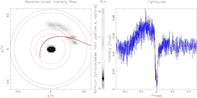
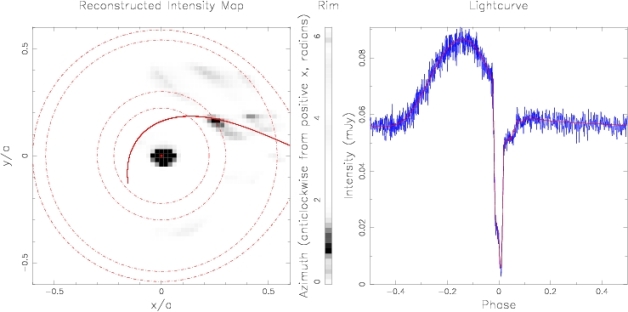
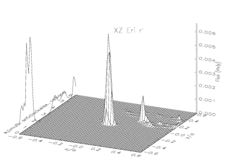
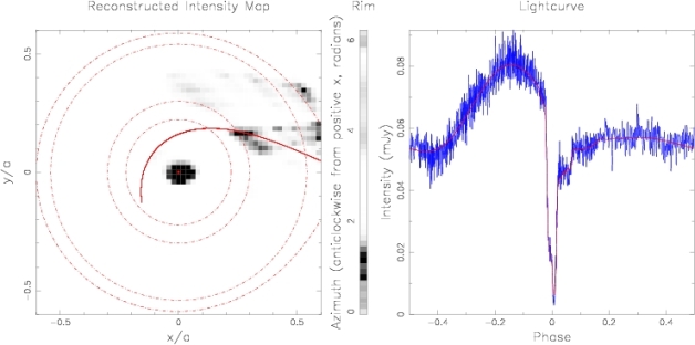
Figure 5.12: As figure 4.7, but for, from top, the u^′, g^′ and r^′ data of XZ Eri. The system parameters adopted for the reconstruction are $q=0.1098$, $i=80.16^{\circ}$ and $R_{\rm d}=0.3a$

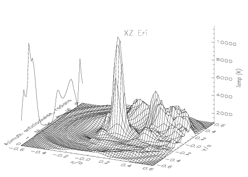
Figure 5.13: 3-dimensional plot of a blackbody fit to the reconstructed disc intensities of XZ Eri shown in figure 5.12.

The eclipse mapping results for DV UMa are shown in figures 5.14. The main features of the reconstructed disc are as follows. The white dwarf and bright spot are evident, with the white dwarf being significantly the brighter of the two. The disc itself is effectively invisible (the numerous small-scale features are most likely spurious remnants of the arcs discussed in § 3.7). The intensity distribution along the disc rim (of radius $0.31805a$; see tables 5.4, 5.5 and 5.6) shows a peak at the location of the bright spot, with smaller features probably due to flickering in the light curve.

The temperature map of the disc of DV UMa shown in figure 5.15 was produced by fitting a blackbody function convolved through the filter response functions to each point in the relevant reconstructed maps. The orbital separation and distance to the system adopted were those derived in § 5.3.2.

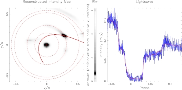
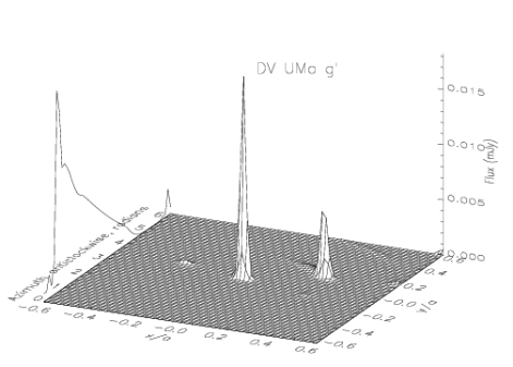
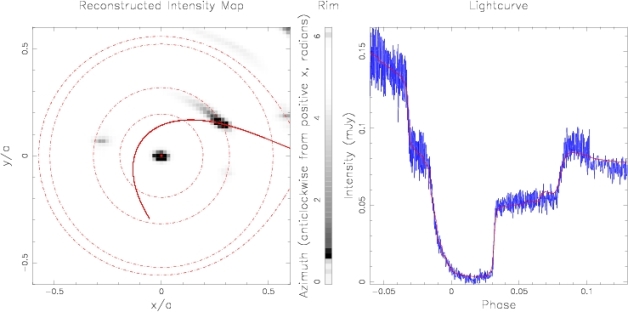
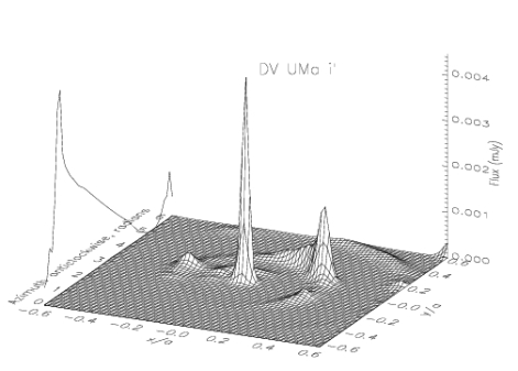
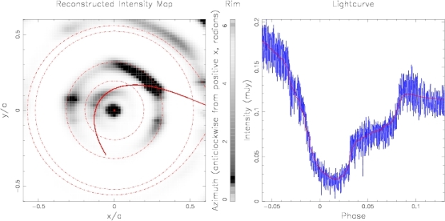
Figure 5.14: As figure 5.12, but for, from top, the u^′, g^′ and i^′ data of DV UMa. The system parameters adopted for the reconstruction are $q=0.1506$, $i=84.24^{\circ}$ and $R_{\rm d}=0.31805a$

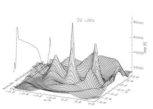
Figure 5.15: 3-dimensional plot of a blackbody fit to the reconstructed disc intensities of DV UMa shown in figure 5.14.

Chapter 6 GY Cnc, IR Com and HT Cas

The contents of this chapter have been accepted for publication in the Monthly Notices of the Royal Astronomical Society as ULTRACAM photometry of the eclipsing cataclysmic variables GY Cnc, IR Com and HT Cas by Feline, Dhillon, Marsh, Watson, & Littlefair (2005). The exceptions to this are the eclipse mapping results for GY Cnc and IR Com presented at the end of this chapter in § 6.4.2. The reduction and analysis of the data are all my own, as is the text below. Dr. Vik Dhillon supervised all work presented here.

GY Cnc (= RX J0909.8+1849 = HS 0907+1902) is a $V\sim 16$ mag eclipsing dwarf nova with an orbital period $P_{{\rm orb}}=4.2$ hr. GY Cnc was detected in both the Hamburg Schmidt objective prism survey (Hagen et al., 1995) and the ROSAT Bright Source catalogue (Voges et al., 1999), and identified as a possible CV by Bade et al. (1998). Spectroscopic and photometric follow-up observations by Gänsicke et al. (2000) confirmed the status of GY Cnc as an eclipsing dwarf nova by detecting it in both outburst and quiescence. Shafter et al. (2000) used multi-colour photometric observations of GY Cnc to determine the temperatures of the white dwarf, bright spot and accretion disc and the disc power-law temperature exponent, which they found to be largely independent of the mass ratio assumed. Spectroscopic and photometric observations obtained by Thorstensen (2000) constrain the mass ratio $q=0.41\pm 0.04$ and the orbital inclination $i=77.0^{\circ}\pm 0.9^{\circ}$ (after applying corrections to the radial velocity of the secondary star $K_{2}$). The spectral type of the secondary star has been estimated as M$3\pm 1.5$ (Gänsicke et al., 2000; Thorstensen, 2000). GY Cnc was observed during decline from outburst in 2001 November by Kato et al. (2002b), who suggest that GY Cnc is an “above-the-gap counterpart” to the dwarf nova HT Cas.

IR Com (= S 10932 Com) was discovered as the optical counterpart to the ROSAT X-ray source RX J1239.5 (Richter & Greiner, 1995). IR Com exhibits high (photographic magnitude ${\rm m}_{\rm ph}=16.5$ mag) and low (${\rm m}_{\rm ph}=18.5$ mag) brightness states (Richter & Greiner, 1995; Richter et al., 1997), with outburst amplitudes of ${\rm m}_{\rm ph}\sim 4.5$ mag (Richter et al., 1997; Kato et al., 2002a). Wenzel et al. (1995) detected eclipses in the light curve of IR Com and determined an orbital period of 2.1 hr, just below the period gap. Richter et al. (1997) present photometric and spectroscopic observations of IR Com, which illustrate the highly variable nature of the target. Kato et al. (2002a) reported observations of IR Com in, and during the decline from, outburst. None of the published light curves of IR Com show much evidence for the presence of an orbital hump before eclipse, or for asymmetry of the eclipse itself (although the limited time-resolution of the observations may mask such asymmetries to an extent). Kato et al. (2002a) again suggest that IR Com is a twin of HT Cas.

HT Cas is a well-known and well-studied eclipsing dwarf nova. It has a quiescent magnitude of $V\sim 16.4$ mag and an orbital period of 1.77 hr. The literature on HT Cas is extensive; here I only discuss a selection of relevant work. The system parameters of HT Cas have been well-determined by Horne et al. (1991) using simultaneous U, B, V and R observations in conjunction with those of Patterson (1981): $q=0.15\pm 0.03$ and $i=81.0^{\circ}\pm 1.0^{\circ}$. In a companion paper, Wood et al. (1992) determined the temperature of the white dwarf ($T=14\,000\pm 1000$ K) and estimated the distance to the system ($D=125\pm 8$ pc). They also eclipse-mapped the accretion disc, illustrating the flat radial temperature profile typical of quiescent dwarf novæ. Vrielmann et al. (2002) have recently reconstructed the temperatures and surface densities of the quiescent accretion disc of HT Cas using physical parameter eclipse mapping. This method also yields an estimate of the distance, $D=207\pm 10$ pc. Marsh (1990) detected the secondary star in HT Cas using low-resolution spectra, estimating the spectral type as M$5.4\pm 0.3$. Marsh (1990) found the secondary star to be consistent with main-sequence values for the mass, radius and luminosity. Robertson & Honeycutt (1996) discuss the long-term quiescent light curve of HT Cas, with particular regard to the (unusual) presence of high- and low-states (at 16.4 and 17.7 mag, respectively). Wood et al. (1995) detected an X-ray eclipse of HT Cas using ROSAT observations during one of the system’s low-luminosity states. The X-rays are believed to originate in a boundary layer between the white dwarf and inner accretion disc.

In this chapter, I present light curves of GY Cnc, IR Com and HT Cas, obtained with ultracam. The data for GY Cnc and IR Com are of the highest time-resolution yet obtained, and are the first simultaneous, three-colour light curves for these objects. I present eclipse maps of HT Cas in quiescence in 2002 and 2003, which show distinct changes in the structure of the accretion disc which are related to the overall brightness of the system.

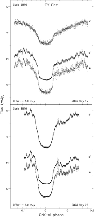
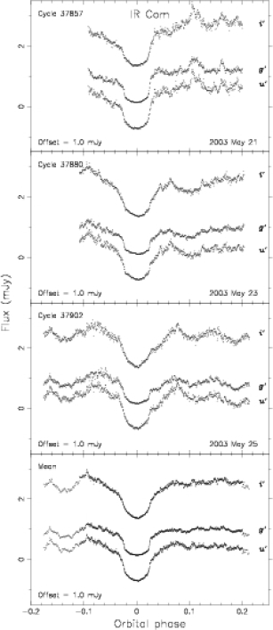
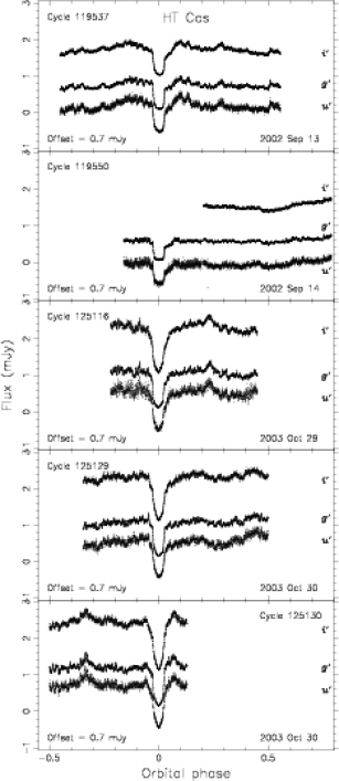
Figure 6.1: Left. The light curves of GY Cnc. Centre. The light curves of IR Com. Right. The light curves of HT Cas. The i^′ and z^′ data are offset vertically upwards and the u^′ data are offset vertically downwards by the amount specified in the relevant plot. Note that the i^′ HT Cas data of 2002 September 14 were lost due to a technical problem with this CCD. The mean light curve of IR Com is also shown.

The observations of GY Cnc, IR Com and HT Cas are summarised in table 2.1, and the data reduction procedure is detailed in § 2.3. The light curves of GY Cnc, IR Com and HT Cas are shown in figure 6.1. A technical problem with the i^′ band CCD destroyed the data in this band on 2002 September 14 (HT Cas). Note also that the timing data of 2003 October 29 (HT Cas) were corrupted. The relative timings remained precise, however, enabling the accurate phasing of the data (see § 6.1).

6.1 Orbital ephemerides

The times of mid-eclipse $T_{{\rm mid}}$ given in table 6.1 were determined as decribed in § 3.2, taking the midpoint of the white dwarf eclipse as the point of mid-eclipse. If the sharp eclipse is caused by the obscuration of the bright spot rather than the white dwarf, then phase zero, as defined by the ephemerides below, may not necessarily correspond to the conjunction of the white and red dwarf components. As discussed in § 6.2–6.4, however, it is probable that the sharp eclipse in all three objects (and certainly HT Cas) is of the white dwarf.

The orbital ephemeris of GY Cnc was determined using the seven eclipse timings of Gänsicke et al. (2000), the eight timings of Shafter et al. (2000), the seven timings of Kato et al. (2000), the two timings of Vanmunster (2000), the four timings of Kato et al. (2002b) and the six ultracam timings determined in this chapter and given in table 6.1. Errors adopted were $\pm 1\times 10^{-4}$ days for the data of Gänsicke et al. (2000) and Shafter et al. (2000), $\pm 5\times 10^{-5}$ days for the data of Kato et al. (2000), Vanmunster (2000) and Kato et al. (2002b) and $\pm 1\times 10^{-5}$ days for the ultracam data. A linear least squares fit to these times gives the following orbital ephemeris for GY Cnc:

$$\begin{array}[]{ccrcrl}\\ HJD&=&2451581.826653&+&0.1754424988&E.\\ &&14&\pm&21&\end{array}$$

Table 6.1: Mid-eclipse timings of GY Cnc, IR Com and HT Cas. The cycle numbers were determined from the ephemerides described in § 6.1. Note that a technical problem with the i^′ CCD corrupted the data during eclipse in this band on 2002 September 14. The timings are accurate to $\pm 1\times 10^{-5}$ days (GY Cnc), $\pm 2\times 10^{-5}$ days (IR Com) and $\pm 5\times 10^{-6}$ days (HT Cas).

Target	UT date at	Cycle	${\rm HJD}+2\,452\,530$
	start of night		u′	g′	i′	z′
GY Cnc	2003 5 19	6826	249.397235	249.397223	–	249.397248
GY Cnc	2003 5 23	6849	253.432215	253.432254	253.432254	–
IR Com	2003 5 21	37857	251.503269	251.503250	251.503194	–
IR Com	2003 5 23	37880	253.505096	253.505153	253.505153	–
IR Com	2003 5 25	37902	255.419890	255.419966	255.419909	–
HT Cas	2002 9 13	119537	1.503015	1.503035	1.502995	–
HT Cas	2002 9 14	119550	2.460443	2.460477	–	–
HT Cas	2003 10 30	125129	413.338089	413.338159	413.338199	–
HT Cas	2003 10 30	125130	413.411832	413.411792	413.411769	–

To determine the orbital ephemeris of IR Com, I used the 24 timings of Richter et al. (1997, as listed in , ), the 14 eclipse timings of Kato et al. (2002a) and those nine, given in table 6.1, determined from the ultracam data. The errors adopted for the data of Richter et al. (1997) and Kato et al. (2002a) were $\pm 1\times 10^{-3}$ days for cycles $-134516$, $-51035$, $-42189$, $-29597$ and $-21531$ and $\pm 5\times 10^{-5}$ days for subsequent cycles, except where stated otherwise by Kato et al. (2002a). Those adopted for the ultracam timings were $\pm 2\times 10^{-5}$ days. The orbital ephemeris of IR Com was determined by a linear least squares fit to the above timings, and is

$$\begin{array}[]{ccrcrl}\\ HJD&=&2449486.4818691&+&0.08703862787&E.\\ &&26&\pm&20&\end{array}$$

To determine the orbital ephemeris of HT Cas I used the 11 mid-eclipse times of Patterson (1981), the 23 times of Zhang et al. (1986), the 15 times of Horne et al. (1991) and the 11 ultracam times given in table 6.1. The times of Patterson (1981), Zhang et al. (1986) and Horne et al. (1991) were assigned errors of $\pm 5\times 10^{-5}$ days and the times in table 6.1 assigned errors of $\pm 5\times 10^{-6}$ days. A linear least squares fit to these times gives the following orbital ephemeris for HT Cas:

$$\begin{array}[]{ccrcrl}\\ HJD&=&2443727.937290&+&0.07364720309&E.\\ &&8&\pm&7&\end{array}$$

The loss of accurate timings for the 2003 October 29 HT Cas data meant that these data were phased according to the orbital period derived above, but with a different zero-point. The zero-point used instead was the mid-point of the observed eclipse. Note that the relative timings for this data remained accurate; the times were merely out by a constant, unknown, offset. The cycle number was accurately determined from the times in the hand-written observing log. This may result in a slight fixed time offset for these data due to the uncertainty in determining the point of mid-eclipse.

These ephemerides were used to phase all of the data.

The $O-C$ diagrams for GY Cnc, IR Com and HT Cas produced using the above ephemerides and times of mid-eclipse are shown in figures 6.2, 6.3 and 6.4, respectively. None shows any convincing evidence for period change.

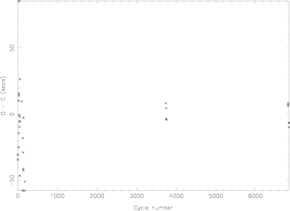
Figure 6.2: The $O-C$ diagram of GY Cnc produced using a linear ephemeris as described in the text.

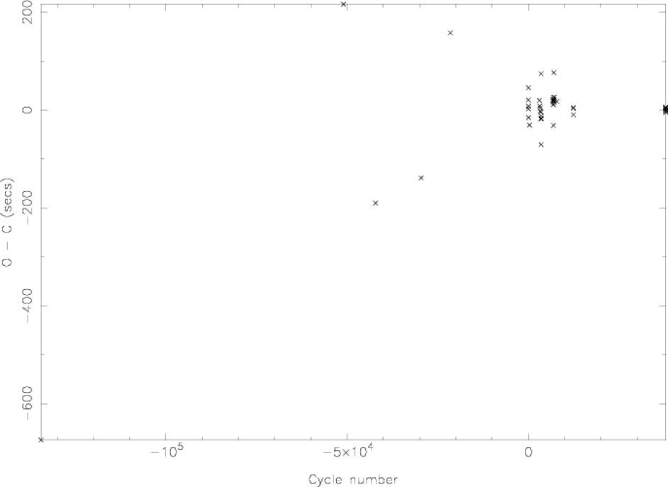
Figure 6.3: The $O-C$ diagram of IR Com produced using a linear ephemeris as described in the text.

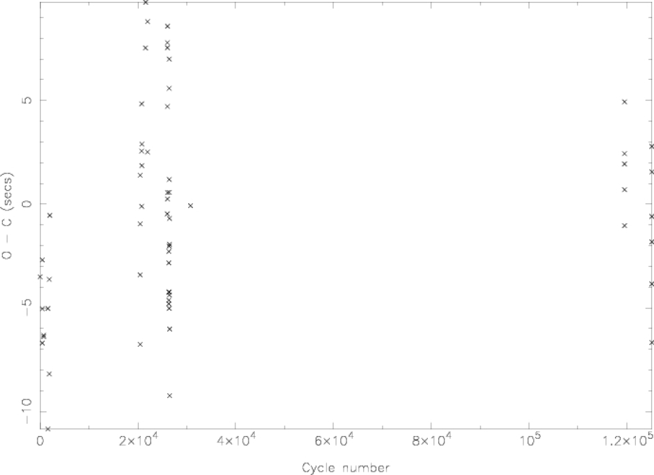
Figure 6.4: The $O-C$ diagram of HT Cas produced using a linear ephemeris as described in the text.

6.2 GY Cnc

In keeping with previous observations (summarised in the introduction to this chapter), the light curve of GY Cnc shown in figure 6.1 shows a deep primary eclipse, with the g^′ flux dropping from a peak value of approximately 3 mJy (15.2 mag) to about 0.6 mJy (17.0 mag) at mid-eclipse. This places the system slightly above its quiescent brightness of $V=16$ mag, shortly after an outburst which reached twelfth-magnitude on 2003 May 13 (Waagen, private communication; observed by the amateur organisation the American Association of Variable Star Observers, AAVSO). The system was therefore likely to still be in decline from outburst. The eclipse morphology appears to be that of a gradual disc eclipse with a sharp eclipse of the white dwarf or bright spot superimposed thereon. The sharp eclipse is most probably that of a white dwarf, not the bright spot, as in both cycles the ingress and egress are of the same order in terms of both duration and depth. The eclipse is flat-bottomed, suggesting that the disc and white dwarf are completely obscured at these phases. The eclipse of the disc appears to be asymmetric, with the ingress being rather sharper than the more gradual egress. This is indicative of asymmetry in the disc structure, possibly due to an extended bright spot at the disc rim. The changing foreshortening of the bright spot, the cause of the orbital hump often observed in other dwarf novæ, would also account for the rather greater flux before eclipse than after. Indeed, the ingress observed on 2003 May 23 appears to show two steps, which I attribute to first the bright spot and then the white dwarf entering eclipse. The likely presence of an extended bright spot is another reason why I suspect that the sharp, discrete eclipse visible in both nights’ data is that of the white dwarf. The light curve of figure 6.1 is morphologically similar to quiescent light curves in the literature (Gänsicke et al., 2000; Shafter et al., 2000; Thorstensen, 2000). These data were not suitable to use for determining the system parameters via either the derivative or lfit techniques. In the first case, the bright spot egress is contaminated by flickering and is too gradual to produce a clear peak in the derivative of the light curve. In the second case, the presence of large-scale flickering prevented the program from locating the ingress and egress points reliably.

Table 6.2: White dwarf contact phases of IR Com, as defined in the text, accurate to $\pm 0.00023$.

Date	Band	$\phi_{{\rm w}1}$	$\phi_{{\rm w}2}$	$\phi_{{\rm w}3}$	$\phi_{{\rm w}4}$	$\phi_{{\rm wi}}$	$\phi_{{\rm we}}$
2003 5 21	u′	–0.031748	–0.020917	0.022841	0.028474	–0.025249	0.024575
	g′	–0.026983	–0.021351	0.021108	0.027174	–0.023517	0.025440
	i′	–0.030015	–0.018318	0.019808	0.028907	–0.025249	0.024575
2003 5 23	u′	–0.027904	–0.021404	0.021487	0.026686	–0.026170	0.025388
	g′	–0.026603	–0.021837	0.021487	0.026253	–0.024003	0.025388
	i′	–0.028770	–0.020971	0.023221	0.025820	–0.021837	0.025388
2003 5 25	u′	–0.027680	–0.020744	0.020848	0.027346	–0.026376	0.024311
	g′	–0.026376	–0.021610	0.022579	0.026913	–0.024645	0.025176
	i′	–0.029844	–0.016411	0.020415	0.026047	–0.022914	0.022579
Mean	u′	–0.027811	–0.022901	0.022448	0.027358	–0.025788	0.025046
light	g′	–0.026077	–0.021744	0.021292	0.027069	–0.023478	0.024758
curve	i′	–0.028965	–0.019722	0.021003	0.027358	–0.027231	0.025625

6.3 IR Com

The light curve of IR Com, shown in figure 6.1, also exhibits a deep primary eclipse. The light curve is highly variable outside of eclipse, with a maximum g^′ flux of about 1.6 mJy (15.9 mag) and a minimum during eclipse of approximately 0.16 mJy (18.4 mag). The average out-of-eclipse g^′ flux level of IR Com during my observations was 1.0 mJy (16.4 mag), consistent with the system being in quiescence. From the light curve of IR Com shown in figure 6.1 it is clear that the light curve of this object is highly variable outside of eclipse. There is a clear eclipse of a compact structure, either the white dwarf or bright spot, as evidenced by the sharpness of the ingress and egress. The highly variable nature of the light curve of IR Com makes it difficult to determine whether the sharp eclipse is of the white dwarf or bright spot. The mean light curve of IR Com shown in figure 6.1 shows the main features of the light curve much more clearly, as flickering is much reduced. The sharp eclipse is revealed to be nearly symmetric, with evidence for an eclipse of the disc in the V-shaped eclipse bottom and the slopes before and after the sharp eclipse. No sign of the eclipse of another compact object is seen, so the sharp eclipse must be of the white dwarf (in which case the bright spot is extremely faint) or an eclipse of the bright spot (in which case the white dwarf remains visible at all phases).

Contact phases of the sharp eclipse of IR Com were determined using the derivative of the light curve, as described in § 3.2. These timings, given in table 6.2, do not show any evidence for asymmetry in the duration of ingress and egress (as is frequently the case with the eclipse of a bright spot, where the ingress is of a longer duration than the egress). Additionally, using the Nauenberg (1972) mass–radius relation for a cold, rotating white dwarf with Kepler’s third law (as described in § 3.5) for reasonable values of $q$ shows that the eclipse contact phases are entirely consistent with the eclipsed object being of the correct size for a white dwarf. As Kato et al. (2002a) point out, their mid-eclipse timings show no significant differences between outburst and quiescence, implying that in both quiescence and outburst the brightness distribution is centred on the white dwarf. These points lead me to believe that the primary eclipse is of the white dwarf, rather than of the bright spot.

No unambiguous bright spot feature is visible in either the individual or mean light curves of IR Com shown in figure 6.1. The absence of a bright spot eclipse prevented the determination of the system parameters via either the derivative or lfit techniques. From the absence of flickering during primary eclipse, it appears that the flickering is confined to the inner regions of the accretion disc or the white dwarf itself. The origin of the flickering in IR Com is most likely the boundary layer between the white dwarf and accretion disc (eclipse mapping of the flickering sources in CVs is discussed in, for example, Bruch, 2000; Baptista & Bortoletto, 2004; Baptista, 2004). The absence of a bright spot eclipse prevented the determination of the system parameters via either the derivative or lfit techniques.

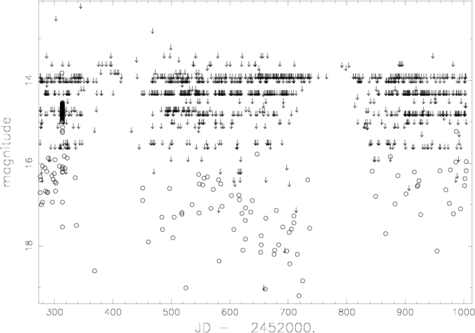
Figure 6.5: The long-term light curve of HT Cas, courtesy of the AAVSO (Waagen, private communication). Open circles are V band observations; arrows mark upper limits on the magnitude of the system. The Julian date scale corresponds to calendar dates from 2002 January 1 to 2004 January 1. Note the outburst in 2002 February, which peaked on 2002 February 6 ($={\rm JD}\;2\,452\,312$).

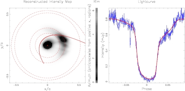
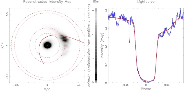
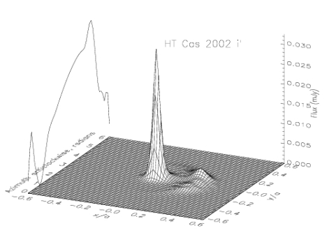
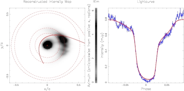
Figure 6.6: As figure 5.12, but for, from top, the u^′, g^′ and i^′ 2002 September 13–14 light curves of HT Cas. The parameters adopted for these reconstructions were those derived by Horne et al. (1991), $q=0.15$ and $i=81.0^{\circ}$. The disc radius was estimated from the position of the reconstructed bright spot, and is $R_{\rm d}=0.28a$. Prior to fitting, a (constant) offset was subtracted from the light curves. This offset was 0.15, 0.09 and 0.32 mJy for the u^′, g^′ and i^′ data, respectively. This offset was 0.15, 0.09 and 0.32 mJy for the u^′, g^′ and i^′ data, respectively. The sharp dip visible at about phase $-0.04$ in the u^′ and g^′ light curves is due to a short gap between observing runs on 2003 September 13 coinciding with a dip in the 2003 September 14 light curve.

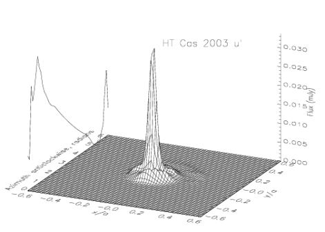
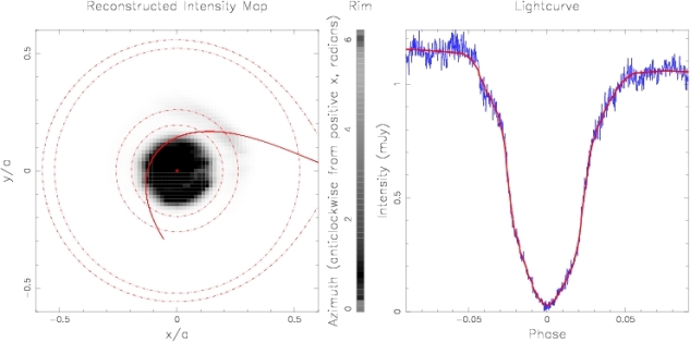
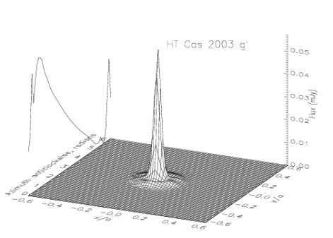
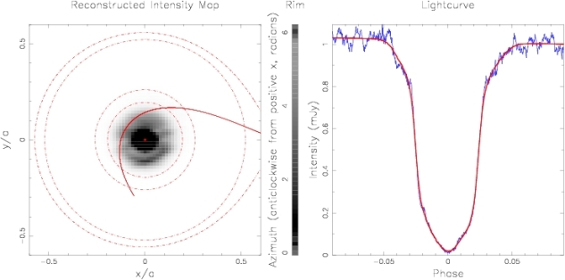
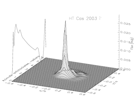
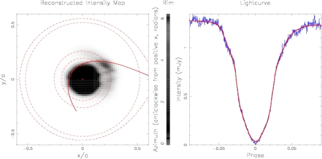
Figure 6.7: As figure 5.12, but for the u^′ (top), g^′ (middle) and i^′ (bottom) 2003 October 29–30 light curves of HT Cas. The radius of the disc (the same as that of the disc rim) was estimated from the position of the bright spot in the eclipse maps, and is $0.26a$. The u^′, g^′ and i^′ light curves were offset vertically by 0.24, 0.14 and 0.42 mJy, respectively.

6.4 HT Cas

6.4.1 Light curve morphology

The light curves of HT Cas shown in figure 6.1 are typical of those found in the literature (e.g. Patterson, 1981; Horne et al., 1991). The typical out-of-eclipse g^′ flux for the 2002 data is 0.7 mJy (16.8 mag), and the typical mid-eclipse g^′ flux is 0.1 mJy (18.9 mag; see also figure 6.6). The peak g^′ flux in the 2002 dataset is approximately 1.0 mJy (16.4 mag). HT Cas is slightly brighter in the 2003 data: the typical out-of-eclipse g^′ flux is 1.2 mJy (16.2 mag), and the mid-eclipse g^′ flux is again about 0.1 mJy (18.9 mag; see also figure 6.7). The 2003 data set is entirely consistent with HT Cas being in its high (brighter) quiescent state (HT Cas exhibits much variability in its quiescent magnitude; see Robertson & Honeycutt, 1996), but the 2002 data appears to be somewhere between the high and low states described therein. The data from 2002 show other clear differences from the data of 2003. First, the eclipse bottoms in 2002 were much flatter than those of 2003, implying that the brightness distribution in 2002 was more centrally concentrated than in 2003. Second, the eclipse depth in 2003 was greater than in 2002, which, as we shall see, is due to increased disc emission and not an increase in the brightness of the white dwarf. There is also visible in the 2002 data a clear shoulder during egress. This appears to be the egress of the bright spot, similar in appearance to the feature seen in the light curves of Patterson (1981). Unfortunately for the aim of determining the system parameters from the eclipse contact phases, no bright spot ingress is visible. This variability of the light curve is typical of HT Cas (e.g. Patterson, 1981; Horne et al., 1991; Robertson & Honeycutt, 1996). The fact that the flux increase between 2002 and 2003 is slight illustrates that these brightness and morphological variations are not due to an overwhelming increase in the disc flux ‘drowning out’ the bright spot, as occurs during outburst. Observations of HT Cas by the AAVSO (Waagen, private communication; figure 6.5) show no evidence for an outburst of HT Cas before the 2003 October observations—the change in the light curve is not due to the system being on the way up or down from an outburst. I term the 2003 and 2002 data the ‘high’ and ‘low’ quiescent states, respectively (although I caution that these probably differ in both underlying cause and detailed observational properties from the various high and low quiescent states discussed in the literature).

6.4.2 Eclipse mapping

The accretion disc of HT Cas was mapped using the techniques described in detail in § 3.7. The data of 2002 and 2003 were mapped independently, since subsequent analysis showed there to be significant differences, discussed below, between the two data epochs.

I have estimated the radius of the disc rim from the position of the reconstructed bright spot, since the disc radius, of $0.28a$ in 2002 and $0.26a$ in 2003, is larger than that derived by Horne et al. (1991) of $0.23a$. I have chosen not to deconvolve and remove the white dwarf from the light curves as the presence of flickering and the lack of a clear distinction between the eclipses of the white dwarf, bright spot and accretion disc make this difficult to do so reliably (see, for example, chapter 5). Besides, clear evidence for the features reproduced in the eclipse maps and discussed below can be seen directly in the light curves themselves.

As only a few light curves were used, the noise in the light curves is dominated by flickering rather than by photon noise. Iterating to a reduced $\chi^{2}=1$ is therefore inappropriate in this case and leads to the noise in the light curves (flickering) being transposed to the eclipse maps. Consequently, the eclipse maps were computed by progressively relaxing the $\chi^{2}$ constraint until the noise in the eclipse maps was satisfactorily ameliorated (as judged by visual inspection).

The reconstructed eclipse maps of HT Cas shown in figures 6.6 and 6.7 show distinct morphological changes from 2002 to 2003. In both 2002 and 2003 the flux comes primarily from the white dwarf, but in 2002 there is clear evidence for a faint bright spot in the outer regions of the accretion disc. The 2003 eclipse maps show a very weak bright spot in the u^′ and i^′ passbands only. The absence of a bright spot in the 2003 g^′ band may, however, be a contrast effect, as the white dwarf is approximately twice as bright in g^′ as in the other bands. Not only is the bright spot much fainter/absent in the 2003 reconstructed maps, but there is evidence for emission from the inner portions of the accretion disc. This is best illustrated by the radial flux profiles shown in figure 6.8. Comparing the two radial profiles to the light curves shown in figure 6.1 demonstrates that the increased emission from the inner disc corresponds to a higher overall brightness state. The greater flux in 2003 is not, upon inspection of the eclipse maps, due to increased emission from the white dwarf, which is actually fainter in 2003 than in 2002, but due to a brighter inner disc.

By summing the flux from each element of each eclipse map whose centre lies within $0.03a$ of the centre of the white dwarf and fitting the resulting colours to the hydrogen-rich, $\log g=8$ white dwarf model atmospheres of Bergeron et al. (1995), converted to the SDSS system using the observed transformations of Smith et al. (2002), the temperature of the white dwarf was determined to be $T_{\rm 1}=15\,000\pm 1000$ K in 2002 and $T_{\rm 1}=14\,000\pm 1000$ K in 2003. Varying the distance from the white dwarf over which the summation took place between $0.01a$–$0.07a$ did not significantly affect the colours and therefore did not significantly affect these temperature estimates. These temperatures are consistent with those found by Wood et al. (1992, $T_{\rm 1}=14\,000\pm 1000$ K) and by Vrielmann et al. (2002, $T_{\rm 1}=15\,500$ K) from the same set of quiescent photometric observations. The effect of the variable nature of the accretion disc of HT Cas is evident in the white dwarf temperatures of HT Cas derived by Wood et al. (1995), of $T_{\rm 1}=13\,200\pm 1200$ K during a low state (which is consistent with these results) and $T_{\rm 1}=18\,700\pm 1800$ K during a normal state (which differs from these results by $\sim 2\sigma$).

In figure 6.9 I present the colour-colour diagrams for the 2002 and 2003 eclipse maps of HT Cas. In both 2002 and 2003 the scatter of the data points from the central regions of the disc ($R/a<0.03$), comprising the white dwarf and boundary layer, is consistent with an increase in the g^′ flux over that expected from a lone white dwarf shifting the position of the data point down and to the left on figure 6.9. This suggests a contribution to this flux from the boundary layer surrounding the white dwarf. This excess g^′ flux is (marginally) more pronounced in 2003 than in 2002, as might be expected given the differences between the distribution of the disc flux for these dates. The emission from both the inner ($0.03\leq R/a<0.18$) and outer ($R/a\geq 0.18$) regions of the disc are concentrated to the right of the blackbody relation in figure 6.9, possibly due to Balmer emission in the u^′ band, suggesting that the disc is optically thin (e.g. Horne & Cook, 1985; Wood et al., 1992; Baptista et al., 1996). There seems to be no significant difference between the colours of the inner and outer discs of 2002 (in 2003 the outer disc was too faint to be plotted on figure 6.9). Interestingly, in both 2002 and 2003, the offset colours (the colours of the flux subtracted from the light curves prior to fitting) lie on the blackbody relation rather than being on the main-sequence curve. A blackbody fit to the 2002 and 2003 offset colours gave $T\sim 11\,000$ K and $T\sim 11\,200$ K, respectively.

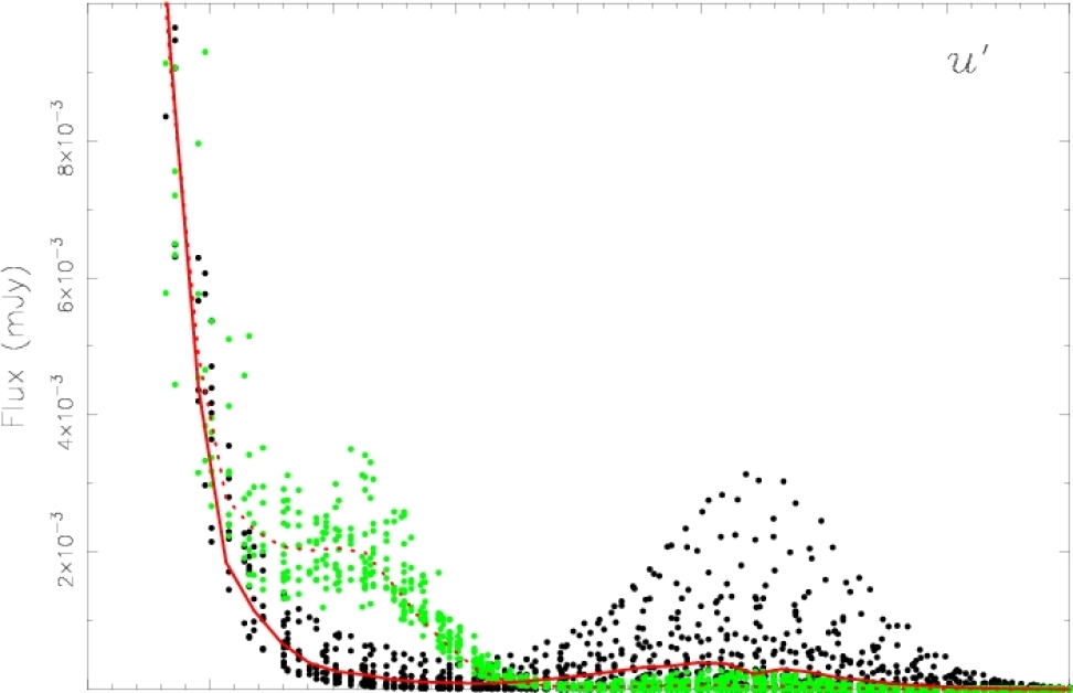
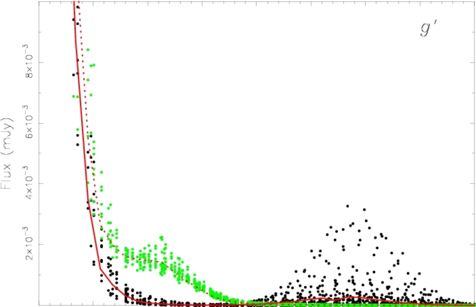
Figure 6.8: The radial flux distribution of the reconstructed accretion disc of HT Cas for the 2002 data (black dots and solid red line) and the 2003 data (green dots and dotted red line). The dots represent the flux and radius of the individual grid elements; the red lines represent the mean flux in concentric annuli. The u^′ and g^′ flux distributions were determined using the data of 2002 September 13–14 and 2003 October 29–30, whereas the i^′ distributions were determined using the data of 2002 September 13 and 2003 October 29–30 (due to a loss of sensitivity in the i^′ chip on 2002 September 14.)

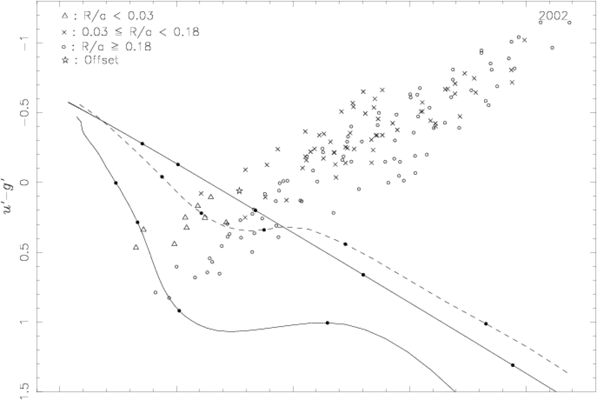
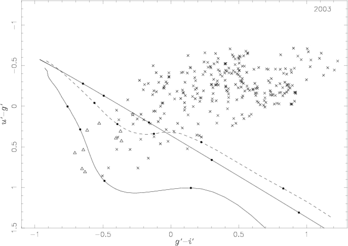
Figure 6.9: Colour-colour diagrams of the accretion disc of HT Cas in (top) 2002 and (bottom) 2003. The solid straight line is a blackbody relationship, the solid curve is the main-sequence relationship of Girardi et al. (2004) and the dashed curve is the white dwarf model atmosphere relation of Bergeron et al. (1995) described in section 3.6. The filled circles superimposed upon each of these lines indicate temperatures of $20\,000$, $15\,000$, $10\,000$, $7000$ and $5000$ K, with the hotter temperatures located at the upper left of the plots (the $5000$ K point for the main-sequence curve lies off the plot). Each of the other points represents one element of the eclipse map. Elements at different radial distances $R$ from the centre of the white dwarf are plotted using different markers, as indicated in the figure. The position of the mid-eclipse (offset) flux is also plotted. In the interests of clarity, only points where the flux in all three passbands was greater than $5\times 10^{-4}$ mJy were plotted.

GY Cnc was eclipse mapped using the system parameters of $q=0.421$ and $i=77.4^{\circ}$. These were calculated from the secondary mass-orbital period relation of Smith & Dhillon (1998), given in equation 1.36, assuming a primary mass of $M_{1}/{\rm M}_{\odot}=1.0$. The orbital inclination was then determined from the eclipse phase width of $\Delta\phi=0.06364\pm 0.00008$ determined from the eclipse timings. For the purposes of modelling the orbital hump using the disc rim, the radius of the accretion disc was assumed to be $R_{{\rm d}}=0.3a$. This value was, arbitrarily, chosen on the basis that it is similar to those of the other dwarf novæ discussed in this thesis, OU Vir, XZ Eri, DV UMa and HT Cas.

As the light curves of IR Com are highly variable, IR Com was eclipse mapped using the mean light curve. The system parameters adopted were $q=0.153$ and $i=81.1^{\circ}$. These were again calculated from the secondary mass-orbital period relation of Smith & Dhillon (1998), assuming a primary mass of $M_{1}/{\rm M}_{\odot}=1.0$. The orbital inclination was then determined from the eclipse phase width of $\Delta\phi=0.0506\pm 0.0003$ determined from the eclipse timings. The radius of the accretion disc was assumed to be $R_{{\rm d}}=0.3a$.

The resulting eclipse maps of GY Cnc and IR Com are shown in figures 6.10 and 6.11, respectively. They show that in both systems the white dwarf dominates the emission from the system, with the accretion disc virtually invisible.

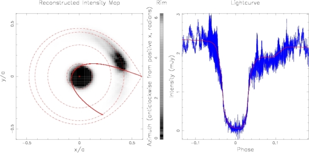
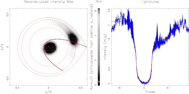
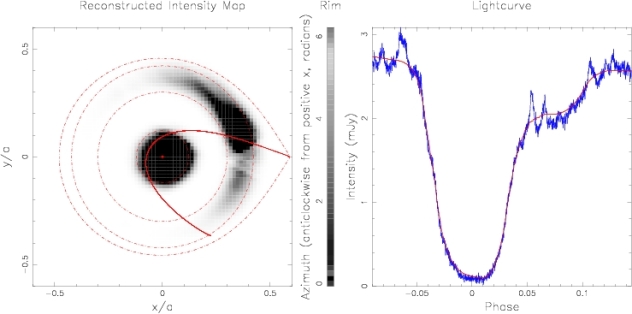
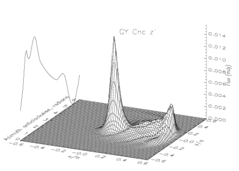
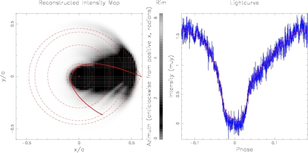
Figure 6.10: As figure 5.12, but for, from top, the u^′, g^′, i^′ and z^′ light curves of GY Cnc. The u^′ and g^′ light curves are of 2003 May 19 and 23 combined, whereas the i^′ and z^′ light curves are of 2003 May 23 and 19, respectively. The system parameters adopted for the reconstruction are $q=0.421$, $i=77.4^{\circ}$ and $R_{\rm d}=0.3a$ (see text for details).

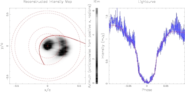
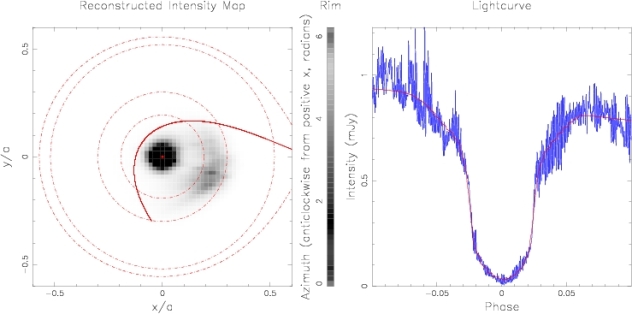
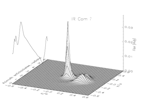
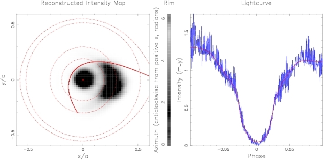
Figure 6.11: As figure 5.12, but for, from top, the u^′, g^′ and i^′ mean light curves of IR Com. The system parameters adopted for the reconstruction are $q=0.153$, $i=81.1^{\circ}$ and $R_{\rm d}=0.3a$ (see text for details).

6.4.3 Temperature maps

The temperature maps of HT Cas shown in figures 6.12 and 6.13 were produced by fitting a blackbody function convolved through the filter response functions to each point in the relevant reconstructed maps. The orbital separation adopted was that derived by Horne et al. (1991), $a/{\rm R_{\odot}}=0.670\pm 0.019$, and the distance to the system was that derived by Wood et al. (1992), $D=125\pm 8{\rm pc}$. Note that, as figure 6.9 illustrates, the disc of HT Cas is not a good approximation to a blackbody in many regions, so the temperature scale in figures 6.12 and 6.13 should be regarded cautiously.

It was not possible to produce meaningful temperature maps of the accretion discs of GY Cnc and IR Com because both the orbital separations and the distances to the systems are currently unknown.

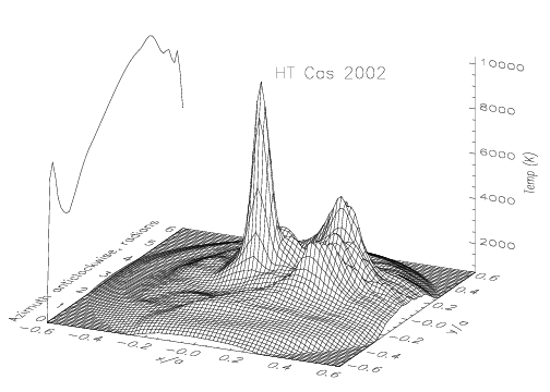
Figure 6.12: 3-dimensional plot of a blackbody fit to the reconstructed 2002 disc intensities of HT Cas shown in figure 6.6.

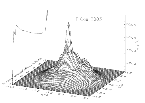
Figure 6.13: 3-dimensional plot of a blackbody fit to the reconstructed 2003 disc intensities of HT Cas shown in figure 6.7.

Chapter 7 Discussion, conclusions and future work

7.1 Discussion and conclusions

7.1.1 OU Vir

I have presented an analysis of 5 eclipses of OU Vir. These eclipses have been used to make the first determination of the system parameters, given in table 4.5. My main conclusions are as follows:

1. Eclipses of both the white dwarf and bright spot were observed during quiescence. The identification of the bright spot ingress and egress appears unambiguous.

2. By requiring the gas stream to pass directly through the light centre of the bright spot the mass ratio and orbital inclination were found to be $q=0.175\pm 0.025$ and $i=79.2^{\circ}\pm 0.7^{\circ}$.

3. Assuming that the central eclipsed object is circular, that its size accurately reflects that of the white dwarf and that it obeys the Nauenberg (1972) approximation to the Hamada & Salpeter (1961) mass-radius relationship, adjusted to $T=21\,700$ K, I find that the white dwarf radius is $R_{1}=0.0097\pm 0.0031\;{\rm R}_{\odot}$ and its mass is $M_{1}=0.90\pm 0.19\;{\rm M}_{\odot}$. This is in good agreement with the mean mass of CV white dwarfs found by Smith & Dhillon (1998) of $\bar{M_{1}}=0.69\pm 0.13\;{\rm M}_{\odot}$.

4. With the same assumptions, I find that the volume radius of the secondary star is $R_{2}=0.181\pm 0.024\;{\rm R}_{\odot}$ and that its mass is $M_{2}=0.16\pm 0.04\;{\rm M}_{\odot}$. The secondary star is therefore consistent with the empirical mass-radius relation for the main-sequence secondary stars in CVs of Smith & Dhillon (1998).

5. A blackbody fit to the white dwarf flux gives a temperature $T_{1}=21\,700\pm 1200$ K and a distance $D=650\pm 210$ pc with the same assumptions as above. These are purely formal errors from the least-squares fit using estimated errors of $\pm 0.01$ mJy for each flux measurement. Given that I use data from only one eclipse, with a single measurement of the flux from each passband, the actual uncertainties are likely to be significantly larger.

6. The accretion disc radius of $R_{{\rm d}}/a=0.2315\pm 0.0150$ is similar in size to that of HT Cas, for which Horne et al. (1991) derived $R_{{\rm d}}/a=0.23\pm 0.03$. This is an unusually small disc radius compared to many other dwarf novæ (e.g. Z Cha, which has $R_{{\rm d}}/a=0.334$; Wood et al., 1989a), but larger than the circularisation radius (Verbunt & Rappaport, 1988, their equation 13) of $R_{{\rm circ}}=0.1820a$. This small disc radius is especially surprising as it was determined from observations obtained only 20 days after the superoutburst was first reported (Kato, 2003).

7. The superhump period of OU Vir is $P_{{\rm sh}}=0.078\pm 0.002$ days (Vanmunster et al., 2000), which means OU Vir lies $5\sigma$ off the superhump period excess-mass ratio relation of Patterson (1998, his equation 8), with the superhump period excess $\epsilon=(P_{{\rm sh}}-P_{{\rm orb}})/P_{{\rm orb}}\sim 0.073$. However, it does not lie on the superhump period excess-orbital period relation either, perhaps indicating that the current estimate of the superhump period $P_{{\rm sh}}$ is inaccurate.

8. The eclipse maps of OU Vir shown in figures 4.7–4.10 show the white dwarf and bright spot to be the main sources of luminosity in the system, and no evidence for the presence of accretion disc emission. They also illustrate the difficulties present in eclipse mapping discrete sources of emission using the maximum entropy technique, especially when combined with the presence of flickering in a single cycle.

7.1.2 XZ Eri and DV UMa

I have presented an analysis of two quiescent eclipses of XZ Eri and three quiescent eclipses of DV UMa. These eclipses have been used to determine the system parameters, given in table 5.7, via two independent methods. The first of these is through analysis of the light curve derivative (Wood et al., 1985, 1986) and the second by fitting a parameterized model of the eclipse (Horne et al., 1994). This is the first determination of the system parameters of XZ Eri. My main conclusions follow:

1. For both objects, separate eclipses of the white dwarf and bright spot were observed. The identification of the bright spot ingress and egress is unambiguous in each case. The eclipse maps of XZ Eri and DV UMa shown in figures 5.12–5.15 show the white dwarf and bright spot to be the main sources of luminosity in these systems, and there is no evidence for the presence of accretion disc emission. Compared to the eclipse maps of OU Vir (figures 4.7–4.10), they also demonstrate the advantages of reducing flickering by phase-folding multiple (similar) cycles.

2. By requiring the gas stream to pass directly through the light centre of the bright spot the mass ratio and orbital inclination were found to be $q=0.117\pm 0.015$ and $i=80.3^{\circ}\pm 0.6^{\circ}$ for XZ Eri and $q=0.148\pm 0.013$ and $i=84.4^{\circ}\pm 0.8^{\circ}$ for DV UMa. The parameterized model of the eclipse yielded $q=0.1098\pm 0.0017$ and $i=80.16^{\circ}\pm 0.09^{\circ}$ for XZ Eri and $q=0.1506\pm 0.0009$ and $i=84.24^{\circ}\pm 0.07^{\circ}$ for DV UMa. The two techniques therefore produce results that are in good agreement with each other. The system parameters of DV UMa have also been estimated by Patterson et al. (2000) using eclipse deconvolution. My analysis is consistent with their findings. The mass ratio I derive for XZ Eri, $q=0.1098\pm 0.0017$, is consistent with XZ Eri being an SU UMa star (Whitehurst, 1988; Whitehurst & King, 1991), as indicated by its (super)outburst history (Woudt & Warner, 2001; Uemura et al., 2004). DV UMa is already confirmed as an SU UMa star after the observation of superhumps in its outburst light curve by Nogami et al. (2001).

3. The empirical mass-radius and mass-period relations for the secondary stars of CVs of Smith & Dhillon (1998) are in good agreement with the values determined here. The results from the parameterized model of XZ Eri give a very low secondary star mass of $M_{2}/{\rm M}_{\odot}=0.0842\pm 0.0024$. This is close to the upper limit on the mass of a brown dwarf, which is $0.072\;{\rm M}_{\odot}$ for objects with solar composition, but can be up to $0.086\;{\rm M}_{\odot}$ for objects with zero metallicity (Basri, 2000). The only dwarf nova with an accurately determined secondary star mass that is less than this is the well-studied system OY Car, which has $M_{2}/{\rm M}_{\odot}=0.070\pm 0.002$ (Wood et al., 1989a). I note also that the orbital period and mass ratio of XZ Eri are similar to those of OY Car (Wood et al., 1989a). As Patterson et al. (2000) note, the spectral type of the secondary star in DV UMa (M4.5; Mukai et al., 1990) implies $M_{2}/{\rm M}_{\odot}=0.12-0.18$ for a main-sequence star of solar metallicity (Chabrier & Baraffe, 1997; Henry et al., 1999), consistent with my results of $0.169\pm 0.023\;{\rm M}_{\odot}$ and $0.157\pm 0.009\;{\rm M}_{\odot}$ for the derivative and model techniques, respectively.

4. Mukai et al. (1990) derive the primary temperature and radius of DV UMa from spectroscopic observations by assuming that the white dwarf emits a blackbody spectrum. The temperature they derive, $T_{1}=22\,000\pm 1500$ K, is consistent with my result of $20\,000\pm 1500$ K. The primary radius ($R_{1}=26\,000-7700$ km) Mukai et al. (1990) calculate is only marginally consistent with my results for the derivative technique ($R_{1}=0.0067\pm 0.0018\;{\rm R}_{\odot}$) and not consistent with the results of the parameterized model ($R_{1}=0.0079\pm 0.0004\;{\rm R}_{\odot}$). This is probably due to the limitation of assuming a blackbody spectrum (Mukai et al., 1990). The white dwarf in DV UMa is unusually massive. My assumption that we are observing a bare white dwarf and not a boundary layer around the primary cannot explain this, as the white dwarf mass derived would in this case be a lower limit (e.g. Feline et al., 2004b). The mass of the white dwarf in XZ Eri is, however, consistent with the mean mass of white dwarfs in dwarf novæ below the period gap derived by Smith & Dhillon (1998).

5. The bright spot scale $SB$ of XZ Eri is constant over all three colour bands. In DV UMa, however, it increases in size as the colour becomes redder. The latter result can be interpreted as follows: the material cools as it moves farther from the impact region between the accretion disc and the gas stream. These results imply that either the time-scale for cooling of the bright spot material is greater for DV UMa than for XZ Eri or that the post-impact material spreads more quickly into the surrounding disc of DV UMa than of XZ Eri. The time-scale for cooling and/or migration of shock-heated material in the bright spot is likely to be affected by factors such as the density and composition of the disc material, the mass ratio of the system and the disc radius.

6. Finally, I note that the system parameters I derive for DV UMa are consistent with the superhump period-mass ratio relation of Patterson (1998, his equation 8). XZ Eri, however, lies $5\sigma$ off this relation. I use here the superhump periods $P_{\rm{sh}}=0.062808\pm 0.000017$ days for XZ Eri (Uemura et al., 2004) and $P_{\rm{sh}}=0.08870\pm 0.00008$ days for DV UMa (Patterson et al., 2000).

7.1.3 GY Cnc, IR Com and HT Cas

I have found that the dwarf novæ GY Cnc and IR Com both exhibit eclipses of the white dwarf, and have a bright spot which is faint (GY Cnc) or undetected (IR Com). I have determined updated ephemerides for both of these objects. IR Com, with its short orbital period, significant flickering, high/low quiescent states (Richter & Greiner, 1995; Richter et al., 1997) and lack of orbital hump or bright spot strongly resembles HT Cas in terms of its photometric behaviour (see also Kato et al., 2002a).

The colours of the offset flux of HT Cas shown in figure 6.9, which is estimated from the flux at mid-eclipse, suggest that it does not originate solely from the secondary star. Marsh (1990) detected the secondary star in HT Cas, and found it to be indistinguishable from a main-sequence star of spectral type M$5.4\pm 0.25$, which lies off to the bottom right of the plot of figure 6.9 on the main-sequence relation. It is unlikely that the mid-eclipse flux is from outer regions of the accretion disc at the back of the disc which remain uneclipsed at phase zero, since examination of the eclipse maps shown in figures 6.6 and 6.7 reveals that the emission from the rest of the disc is restricted to either the bright spot (in 2002) or the inner disc (in 2003). Given this, my preferred explanation for the mid-eclipse colours of HT Cas is that they are a combination of flux from the secondary star (which dominates in the i^′ band) and flux from a vertically extended, optically thin disc wind, whose Balmer emission causes it to dominate in the u^′ band. I note that the offset flux level seems to be correlated with the flux from the inner regions of the accretion disc, which supports the hypothesis of a disc wind originating from the inner disc region or boundary layer of HT Cas. I caution, however, that systematic errors may affect the offset fluxes due to the technique used to determine them, and that this conclusion is therefore tentative. (As the offset flux is a small fraction of the total light, except in the i^′ band, any systematic errors present in the offset fluxes will not significantly affect the rest of these results.)

The eclipse maps of HT Cas shown in figures 6.6 and 6.7 and the radial flux profiles shown in figure 6.8 clearly demonstrate that the accretion disc of HT Cas was in two distinct states during the 2002 and 2003 observations. In the 2002 data the disc provided a negligible contribution to the total light, except for the presence of a bright spot in its outer regions. In 2003 the bright spot was much fainter, but the inner disc was luminous, causing the overall system brightness to be $\sim 0.6$ mJy brighter than in 2002. The uneclipsed component was also slightly brighter in 2003 than 2002 (probably due to variability of the secondary star; see captions to figures 6.6 and 6.7), but was not the major cause of the differences in the flux. I proceed to review previous observations and to discuss various possible explanations for this behaviour.

The most likely reasons for the observed changes in the intensity distribution of the quiescent accretion disc of HT Cas lie in variability of the secondary star (which supplies the disc with material) or some property of the accretion disc itself. We can exclude the white dwarf as the cause of the variability since the only plausible way that this could affect the majority of the disc is via a magnetic field. HT Cas is a confirmed dwarf nova, whose white dwarfs do not have magnetic fields strong enough to significantly influence the motion of gas in the disc (e.g. Warner, 1995).

The most obvious mechanism for the accretion disc to produce the observed behaviour of HT Cas is via some relationship to the outburst cycle. Baptista & Catalán (2001) reported changes in the structure of the accretion disc of EX Dra (a dwarf nova above the period gap) through its outburst cycle, specifically the presence of a low-brightness state immediately after outburst during which the disc and bright spot were exceptionally faint. In EX Dra, the low-brightness state is due to reduced emission from all parts of the disc and white dwarf; the eclipse maps of HT Cas presented in figures 6.6–6.8, however, demonstrate that the quiescent luminosity of HT Cas is affected by which areas of the disc are luminous. Robertson & Honeycutt (1996) find that both the transition between the quiescent high and low states and the duration of the low state in HT Cas occur on time-scales of days to months compared to the outburst cycle length of $\sim 400$ days (Wenzel, 1987). Truss, Wynn, & Wheatley (2004) proposed a (slowly cooling) hot inner region of the disc in order to explain the constant quiescent brightness observed in (most) dwarf novæ, which is contrary to the increase of 1–3 magnitudes predicted by most disc instability models (see Lasota, 2001 for a review). This fails to account for the observed changes in the outer accretion disc of HT Cas, but does provide a plausible explanation for the variability of the inner regions of the disc. This model, however, necessitates an outburst between the two sets of observations reported here, which amateur observations (figure 6.5) can neither confirm nor refute. I conclude that this latter scenario is the only plausible way in which the changes in the accretion disc of HT Cas could be related to its position in the outburst cycle.

The secondary star can also induce changes in the accretion disc. For example, variability of the rate of mass transfer from the secondary star is often (plausibly) cited as a mechanism to explain the quiescent variability of dwarf novæ (and other CVs). Baptista & Bortoletto (2004) observed the short-period dwarf nova V2051 Oph in high and low quiescent states. Eclipse maps showed that the increased emission in the high state was due to greater emission from the bright spot and gas stream region, implying a higher mass transfer rate from the secondary star. Interestingly, this is the opposite to what I find for HT Cas.

Variability of the secondary star is in fact the mechanism usually proposed to explain the well-documented presence of high/low quiescence states in HT Cas (e.g. Berriman et al., 1987, Wood, 1995; Robertson & Honeycutt, 1996). The most frequently cited explanation is that suggested by Livio & Pringle (1994), of star spots passing over the inner Lagrangian point temporarily lowering the mass transfer rate from the secondary star. Another possible causal process is magnetic variability of the secondary star. Ak et al. (2001) found cyclical variations in the quiescent magnitudes and outburst intervals of 22 CVs, which they attributed to solar-type magnetic activity cycles of the secondary stars. This can result in an increased mass transfer rate from the secondary star as well as the removal of angular momentum from the outer regions of the disc, causing material to accumulate in the inner regions of the disc rather than in the outer regions. The magnetic activity cycle of the secondary stars derived by Ak et al. (2001) is, however, on the wrong time-scale (years) to explain the frequency of the high/low state transitions and durations (days/months) observed by Robertson & Honeycutt (1996).

In summary, variations in the rate of mass transfer from the secondary star can explain the variability of the bright spot, but fail to account for the changes in the inner disc. These can be explained by a larger mass transfer rate through the accretion disc (possibly due to a rise in the disc viscosity and/or the scenario proposed by Truss et al., 2004) increasing the emission from the inner disc via viscous dissipation.

I conclude that the variability of the quiescent accretion disc of HT Cas is caused by variations both in the rate of mass transfer from the secondary star and through the accretion disc. An increase in the viscosity of the accretion disc leading to an increase in the rate of mass transfer through the disc cannot explain these results alone. Such a viscosity increment would spread material both inwards and outwards, meaning that, although this scenario could explain the rise in the 2003 inner disc flux, one would still expect to observe a bright spot at the intersection of the outer disc and gas stream. In the 2002 observations then, the rate of mass transfer through the disc was lower and the rate of mass transfer from the secondary star greater than in 2003. It is clearly desirable to undertake long-term monitoring of HT Cas (or a similar object, e.g. IR Com) with the aim of eclipse mapping the changes that occur in the disc during quiescence and especially during a transition between the high and low states in order to determine the triggers and physical mechanisms underlying this behaviour.

7.2 Overview

The work contained in this thesis has increased the number of accurately known CV masses by three. As of 1998, there were only 14 reliable mass determinations of CV secondary stars (Smith & Dhillon, 1998). This work forms part of a long term project at Sheffield that aims to increase this number (e.g. Smith & Dhillon, 1998; Thoroughgood et al., 2001, 2004, 2005; Thoroughgood, 2005; Feline et al., 2004a, b, c). Since the review of Smith & Dhillon (1998), there have been at least eleven accurate mass determinations of CVs, to whit: OU Vir (Feline et al., 2004b, c); XZ Eri and DV UMa (Feline et al., 2004a); U Sco (Thoroughgood et al., 2001); AC Cnc and V363 Aur (Thoroughgood et al., 2004); V347 Pup (Thoroughgood et al., 2005); WZ Sge (Skidmore et al., 2002); IY UMa (Steeghs et al., 2003); HS 0907+1902 (Thorstensen, 2000); EX Dra (Baptista et al., 2000); and U Gem (Long & Gilliland, 1999; Naylor et al., 2005). Figure 7.1 shows the results from the work contained in this thesis for the secondary star masses and orbital periods of OU Vir, XZ Eri and DV UMa compared to the empirical mass-period relations given in equation 1.35 and obtained by Smith & Dhillon (1998, equation 1.36).

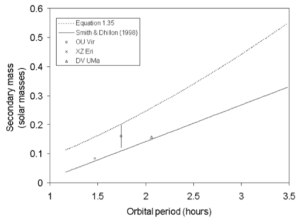
Figure 7.1: The secondary star masses and orbital periods for OU Vir, XZ Eri and DV UMa determined in this thesis, compared to the empirical mass-period relations given in equation 1.35 and obtained by Smith & Dhillon (1998, equation 1.36). The error bars on the orbital periods of OU Vir, XZ Eri and DV UMa and on the secondary star masses of XZ Eri and DV UMa are of the order of the size of the symbols used to plot the points, and so are not plotted.

As discussed in § 1.6, accurate measurements of the masses of CVs are important for many reasons.

The common envelope theory of stellar evolution (see § 1.4.3 and Iben & Livio, 1993), for example, requires reliable endpoint masses—those of CVs—in order to test computational models. Kolb (1993) finds that 70 per cent of all CVs should be systems that have evolved to contain brown dwarfs, whereas the models of Politano (2004) predict that $\sim 18$ per cent of the zero-age CV population will contain a brown dwarf secondary star. The models may differ in their predictions of the exact fraction of systems with brown dwarf secondary stars, but they agree that the number is significant. This figure is highly dependent on the efficiency of the common envelope in removing the orbital energy of the pre-CV, the initial mass ratio distribution of the CV population and the details of the disrupted magnetic braking model. The detection of a brown dwarf secondary star would be a crucial step in understanding the evolutionary processes that have formed the current CV population. Unfortunately, searches for CVs with brown dwarf secondaries (e.g Mennickent et al., 2004) have yet to find direct evidence for such systems, although several candidates exist for which there is “significant indirect evidence” for a brown dwarf secondary star (Littlefair et al., 2003). The secondary stars in CVs are often faint and undetectable spectroscopically (see Littlefair et al., 2003), rendering unlikely the measurement of the radial velocity of the secondary star. One would expect systems that have evolved to near the minimum period to have a low mass-transfer rate and hence a faint accretion disc, allowing the bright spot and white dwarf eclipses to be clearly observed. The results contained in this thesis (especially those for XZ Eri) demonstrate that the photometric technique works well for systems near the period minimum where we expect to find these objects. The photometric method of mass determination described in this thesis is the only unambiguous method of detecting a brown dwarf secondary star in a CV.

The disrupted magnetic braking model (discussed in § 1.4.7), the currently favoured mechanism for the origin of the period gap, also needs accurate secondary star masses for observational confirmation. In this model, the secondary stars in CVs change from being out of thermal equilibrium and hence under-massive for their radii above the period gap to thermally relaxed (i.e. in thermal equilibrium) below the period gap. This should produce a ‘kink’ in the mass–radius plot for the secondary stars of CVs (see figure 7.2 and Smith & Dhillon, 1998), which cannot currently be seen due to two reasons: first, the scarcity of mass measurements, and second, the inaccuracy of many of these measurements. The three mass determinations contained within this thesis are consistent with the secondary star mass-radius relation of Smith & Dhillon (1998, see also figure 7.2).

7.3 Future work

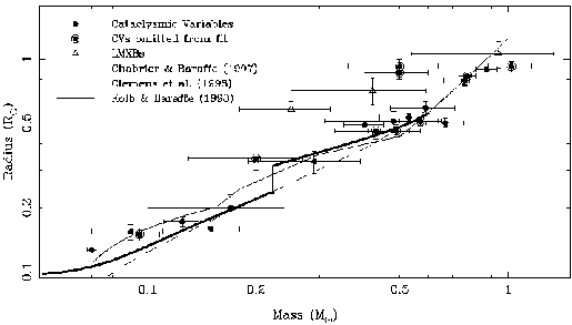
Figure 7.2: The masses and radii of the secondary stars in CVs and LMXBs. The filled circles are data for CVs; those which are ringed were excluded from the fit. The open triangles are data for low mass X-ray binaries (LMXBs). The theoretical models of Chabrier & Baraffe (1997, the dashed line) and the empirical relation derived by Clemens et al. (1998, the thin solid line) are plotted. The thick solid line shows the secular evolution of the mass and radius of the secondary star computed by Kolb & Baraffe (1999, described in the figure as Kolb & Baraffe 1998). From Smith & Dhillon (1998). The secondary star masses and radii determined in this thesis are, for comparison: OU Vir, $M_{2}/{\rm M}_{\odot}=0.16\pm 0.04$ and $R_{2}/{\rm R}_{\odot}=0.177\pm 0.024$; XZ Eri, $M_{2}/{\rm M}_{\odot}=0.0842\pm 0.0024$ and $R_{2}/{\rm R}_{\odot}=0.1315\pm 0.0019$; DV UMa, $M_{2}/{\rm M}_{\odot}=0.157\pm 0.004$ and $R_{2}/{\rm R}_{\odot}=0.2022\pm 0.0018$. All three lie within the scatter of the points.

More candidate systems for photometric mass determinations are constantly being discovered. The Sloan Digital Sky Survey (SDSS) has already uncovered many excellent candidates (Szkody et al., 2002, 2003, 2004). The number of previously unknown CVs discovered by the SDSS is expected to number about 400 systems, most of which will be faint, low mass transfer rate systems, ideal for the above purposes. Candidate systems are also being uncovered by the Hamburg Quasar Survey (Hagen et al., 1995; Araujo-Betancor et al., 2005). This thesis has demonstrated that the photometric method is an essential tool for accurate mass determinations of the many faint, short period, eclipsing dwarf novæ that will be uncovered by surveys such as these.

An attractive future project with ultracam is the long-term monitoring of dwarf novæ. Future plans for ultracam include mounting it on the 2-m class Aristarchos and Isaac Newton (INT) telescopes in Greece and La Palma, respectively. The combination of ultracam with either of these telescopes would be ideal for such long-term monitoring. Observing time for such a long-term project would be difficult to obtain on larger telescopes, and the above combinations of ultracam and either Aristarchos or the INT would in any case be able to achieve sufficient signal-to-noise and time resolution to map the accretion discs of bright CVs in detail. Of particular interest are changes in the accretion disc through the outburst cycle (e.g. Baptista & Catalán, 2001) and the physical mechanisms underlying the existence of high and low quiescent states in several short-period dwarf novæ (see chapter 6 and Feline et al., 2005). It might be hoped that detailed eclipse mapping through the outburst cycle of a dwarf nova would reveal heating/cooling fronts running from the outer to the inner regions of the accretion disc or vice versa (see Warner, 1995, and references therein for a detailed discussion). Doppler tomography, a technique which produces Doppler maps of the system, also holds promise in this regard. For example, Steeghs (2004) observed WZ Sge through its 2001 outburst, producing movies of the evolving accretion flow. The detection of such heating and cooling fronts would provide an invaluable observational framework in which to hang improved theory of the underlying physics of accretion discs.

References

- Ak et al. (2001) Ak, T., Ozkan, M. T., & Mattei, J. A. 2001, A&A, 369, 882
- Allan et al. (1996) Allan, A., Hellier, C., & Ramseyer, T. F. 1996, MNRAS, 282, 699
- Andronov & Pinsonneault (2004) Andronov, N. & Pinsonneault, M. 2004, ApJ, 614, 326
- Andronov et al. (2003) Andronov, N., Pinsonneault, M., & Sills, A. 2003, ApJ, 582, 358
- Araujo-Betancor et al. (2005) Araujo-Betancor, S., Gänsicke, B. T., Hagen, H.-J., Marsh, T. R., Harlaftis, E. T., Thorstensen, J., Fried, R. E., Schmeer, P., & Engels, D. 2005, A&A, 430, 629
- Baba et al. (2002) Baba, H., Sadakane, K., Norimoto, Y., Ayani, K., Ioroi, M., Matsumoto, K., Nogami, D., Makita, M., & Taichi, K. 2002, PASJ, 54, L7
- Bade et al. (1998) Bade, N., Engels, D., Voges, W., Beckmann, V., Boller, T., Cordis, L., Dahlem, M., Englhauser, J., Molthagen, K., Nass, P.and Studt, J., & Reimers, D. 1998, A&AS, 127, 145
- Bailey (1979) Bailey, J. A. 1979, MNRAS, 187, 645
- Balbus & Hawley (1991) Balbus, S. A. & Hawley, J. F. 1991, AJ, 376, 214
- Baptista (2001) Baptista, R. 2001, in Astrotomography: Indirect Imaging Methods in Observational Astronomy, ed. H. M. J. Boffin, D. Steeghs, & J. Cuypers (Berlin: Springer-Verlag Lecture Notes in Physics), 307
- Baptista (2004) Baptista, R. 2004, 325, 181
- Baptista & Bortoletto (2004) Baptista, R. & Bortoletto, A. 2004, AJ, 128, 411
- Baptista & Catalán (2001) Baptista, R. & Catalán, M. S. 2001, MNRAS, 324, 599
- Baptista et al. (2000) Baptista, R., Catalán, M. S., & Costa, L. 2000, MNRAS, 316, 529
- Baptista et al. (1998) Baptista, R., Catalán, M. S., Horne, K., & Zilli, D. 1998, MNRAS, 300, 233
- Baptista et al. (1995) Baptista, R., Horne, K., Hilditch, R. W., Mason, K. O., & Drew, J. E. 1995, ApJ, 448, 395
- Baptista & Steiner (1993) Baptista, R. & Steiner, J. E. 1993, A&A, 277, 331
- Baptista et al. (1996) Baptista, R., Steiner, J. E., & Horne, K. 1996, MNRAS, 282, 99
- Basri (1987) Basri, G. 1987, ApJ, 316, 377
- Basri (2000) —. 2000, ARA&A, 38, 485
- Bath & Pringle (1981) Bath, G. T. & Pringle, J. E. 1981, MNRAS, 194, 967
- Beard et al. (2002) Beard, S., Vick, A., Atkinson, D., Dhillon, V., Marsh, T., McLay, S., Stevenson, M., & Tierney, C. 2002, in Proc. SPIE 4848, Advanced Telescope and Instrumentation Control Software II
- Beekman et al. (2000) Beekman, G., Somers, M., Naylor, T., & Hellier, C. 2000, MNRAS, 318, 9
- Bergeron et al. (1995) Bergeron, P., Wesemael, F., & Beauchamp, A. 1995, PASP, 107, 1047
- Berriman et al. (1983) Berriman, G., Beattie, D. H., Gatley, I., Lee, T. J., Mochnacki, S. W., & Szkody, P. 1983, MNRAS, 204, 1105
- Berriman et al. (1987) Berriman, G., Kenyon, S., & Boyle, C. 1987, AJ, 94, 1291
- Bobinger et al. (1997) Bobinger, A., Horne, K., Mantel, K.-H., & Wolf, S. 1997, A&A, 327, 1023
- Bruch (2000) Bruch, A. 2000, A&A, 359, 998
- Caillault & Patterson (1990) Caillault, J.-P. & Patterson, J. 1990, AJ, 100, 825
- Cannizzo et al. (1988) Cannizzo, J. K., Shafter, A. W., & Wheeler, J. C. 1988, ApJ, 333, 227
- Chabrier & Baraffe (1997) Chabrier, G. & Baraffe, Y. 1997, A&A, 327, 1039
- Claret & Hauschildt (2003) Claret, A. & Hauschildt, P. H. 2003, A&A, 412, 241
- Clemens et al. (1998) Clemens, J. C., Reid, I. N., Gizis, J. E., & O’Brien, M. 1998, ApJ, 496, 352
- de Kool (1992) de Kool, M. 1992, A&A, 261, 188
- Dhillon (1990) Dhillon, V. S. 1990, PhD thesis, University of Sussex
- Dhillon & Marsh (2001) Dhillon, V. S. & Marsh, T. R. 2001, New Ast. Rev., 45, Issue 1-2, 91
- Dhillon et al. (2005) Dhillon, V. S., Marsh, T. R., & et al. 2005, MNRAS, in preparation
- Dhillon et al. (1991) Dhillon, V. S., Marsh, T. R., & Jones, D. H. P. 1991, MNRAS, 252, 342
- Duerbeck (1992) Duerbeck, H. W. 1992, MNRAS, 258, 629
- Eggleton (1983) Eggleton, P. P. 1983, ApJ, 268, 368
- Feline et al. (2004a) Feline, W. J., Dhillon, V. S., Marsh, T. R., & Brinkworth, C. S. 2004a, MNRAS, 355, 1
- Feline et al. (2004b) Feline, W. J., Dhillon, V. S., Marsh, T. R., Stevenson, M. J., Watson, C. A., & Brinkworth, C. S. 2004b, MNRAS, 347, 1173
- Feline et al. (2004c) —. 2004c, MNRAS, 354, 1279
- Feline et al. (2005) Feline, W. J., Dhillon, V. S., Marsh, T. R., Watson, C. A., & Littlefair, S. P. 2005, MNRAS, in press
- Fiedler et al. (1997) Fiedler, H., Barwig, H., & Mantel, K. H. 1997, A&A, 327, 173
- Flannery (1975) Flannery, B. P. 1975, MNRAS, 170, 325
- Frank et al. (1985) Frank, J., King, A. R., & Raine, D. J. 1985, Accretion Power in Astrophysics (Cambridge: Cambridge University Press)
- Friend et al. (1990) Friend, M. T., Martin, J. S., Smith, R. C., & Jones, D. H. P. 1990, MNRAS, 246, 637
- Fukugita et al. (1996) Fukugita, M., Ichikawa, T., Gunn, J. E., Doi, M., Shimasaku, K., & Schneider, D. P. 1996, AJ, 111, 1748
- Gänsicke et al. (2000) Gänsicke, B. T., Fried, R. E., Hagen, H.-J., Beuermann, K., Engels, D., Hessman, F. V., Nogami, D., & Reinsch, K. 2000, A&A, 356, L79
- Girardi et al. (2004) Girardi, L., Grebel, E. K., Odenkirchen, M., & Chiosi, C. 2004, A&A, 422, 205
- Groot (2001) Groot, P. J. 2001, ApJ, 551, L89
- Gull & Skilling (1989) Gull, S. F. & Skilling, J. 1989, Quantified Maximum Entropy MEMSYS 3 Users’ Manual, User manual, Maximum Entropy Data Consultants Ltd
- Gull & Skilling (1991) —. 1991, Quantified Maximum Entropy MEMSYS 5 Users’ Manual, User manual, Maximum Entropy Data Consultants Ltd
- Hagen et al. (1995) Hagen, H.-J., Groote, D., Engels, D., & Reimers, D. 1995, A&AS, 111, 195
- Hamada & Salpeter (1961) Hamada, T. & Salpeter, E. E. 1961, ApJ, 134, 683
- Hawley & Balbus (1991) Hawley, J. F. & Balbus, S. A. 1991, AJ, 376, 223
- Hellier (2001) Hellier, C. 2001, Cataclysmic Variable Stars: How and Why They Vary (UK: Springer-Verlag)
- Henry et al. (1999) Henry, T. J., Franz, O. G., Wasserman, L. H., Benedict, G. F., Shelus, P. J., Ianna, P. A., Kirkpatrick, J. D., & McCarthy, D. W. 1999, ApJ, 512, 864
- Hind (1856) Hind, J. R. 1856, MNRAS, 16, 56
- Horne (1985) Horne, K. 1985, MNRAS, 213, 129
- Horne & Cook (1985) Horne, K. & Cook, M. C. 1985, MNRAS, 214, 307
- Horne et al. (1994) Horne, K., Marsh, T. R., Cheng, F. H., Hubeny, I., & Lanz, T. 1994, ApJ, 426, 294
- Horne & Stiening (1985) Horne, K. & Stiening, R. F. 1985, MNRAS, 216, 933
- Horne et al. (1986) Horne, K., Wade, R. A., & Szkody, P. 1986, MNRAS, 219, 791
- Horne et al. (1993) Horne, K., Welsh, W. F., & Wade, R. A. 1993, ApJ, 410, 357
- Horne et al. (1991) Horne, K., Wood, J. H., & Steining, R. F. 1991, ApJ, 378, 271
- Howell et al. (1988) Howell, S. B., Mason, K. O., Reichart, G. A., Warnock, A., & Kreidl, T. J. 1988, MNRAS, 233, 79
- Howell et al. (1991) Howell, S. B., Szkody, P., Kreidl, T. J., & Dobrzycka, D. 1991, PASP, 103, 300
- Iben & Livio (1993) Iben, I. & Livio, M. 1993, PASP, 105, 1373
- Joergens et al. (2000) Joergens, V., Spruit, H. C., & Rutten, R. G. M. 2000, A&A, 356, L33
- Kato (2003) Kato, T. 2003, vsnet-alert, No. 7733
- Kato et al. (2002a) Kato, T., Baba, H., & Nogami, D. 2002a, PASJ, 54, 79
- Kato et al. (2002b) Kato, T., Ishioka, R., & Uemura, M. 2002b, PASJ, 54, 1023
- Kato et al. (2000) Kato, T., Uemura, M., Schmeer, P., Garradd, G., Martin, B., Maehara, H., Kinnunen, T., & Watanabe, T. 2000, Inf. Bull. var. Stars, 4873
- King (1988) King, A. R. 1988, QJRAS, 29, 1
- King (1985) King, D. L. 1985, Atmospheric Extinction at the Roque de los Muchachos Observatory, La Palma, RGO/La Palma Technical Note 31
- Knigge et al. (2000) Knigge, C., Long, K. S., Hoard, D. W., Szkody, P., & Dhillon, V. S. 2000, ApJ, 539, L49
- Koester & Schönberner (1986) Koester, D. & Schönberner, D. 1986, A&A, 154, 125
- Kolb (1993) Kolb, U. 1993, A&A, 271, 149
- Kolb & Baraffe (1999) Kolb, U. & Baraffe, I. 1999, MNRAS, 309, 1034
- Kraft (1959) Kraft, R. P. 1959, ApJ, 130, 110
- Kraft (1962) —. 1962, ApJ, 135, 408
- Kristensen (1998) Kristensen, L. K. 1998, Astron. Nachr., 3, 193
- Kruszewski (1966) Kruszewski, A. 1966, Adv. Astr. Astrophys., 4, 233
- Lampton et al. (1976) Lampton, M., Margon, B., & Bowyer, S. 1976, ApJ, 208, 177
- Landau & Lifschitz (1958) Landau, L. & Lifschitz, E. 1958, The Classical Theory of Fields (Oxford: Pergamon)
- Lasota (2001) Lasota, J. P. 2001, New Ast. Rev., 45, 449
- Littlefair (2001) Littlefair, S. P. 2001, PhD thesis, University of Sheffield
- Littlefair et al. (2003) Littlefair, S. P., Dhillon, V. S., & Martín, E. L. 2003, MNRAS, 340, 264
- Livio & Pringle (1994) Livio, M. & Pringle, J. E. 1994, ApJ, 427, 956
- Long & Gilliland (1999) Long, K. S. & Gilliland, R. L. 1999, ApJ, 511, 916
- Lubow & Shu (1975) Lubow, S. H. & Shu, F. H. 1975, ApJ, 198, 383
- Lubow & Shu (1976) —. 1976, ApJ, 207, L53
- Lucy (1967) Lucy, L. B. 1967, Z. Astrophysik, 65, 89
- Lynden-Bell & Pringle (1974) Lynden-Bell, D. & Pringle, J. E. 1974, MNRAS, 168, 603
- Marsh (1990) Marsh, T. R. 1990, ApJ, 357, 621
- Marsh et al. (1987) Marsh, T. R., Horne, K., & Shipman, H. L. 1987, MNRAS, 225, 551
- Mason et al. (2002) Mason, E., Howell, S. B., Szkody, P., Harrison, T. E., Holtzman, J. A., & Hoard, D. W. 2002, A&A, 396, 633
- McClintock et al. (1983) McClintock, J. E., Petro, L. D., Remillard, R. A., & Ricker, G. R. 1983, ApJ, 266, L27
- Mennickent et al. (2004) Mennickent, R. E., Diaz, M. P., & Tappert, C. 2004, MNRAS, 347, 1180
- Mineshige & Wood (1989) Mineshige, S. & Wood, J. H. 1989, MNRAS, 241, 259
- Moffat (1969) Moffat, A. F. J. 1969, A&A, 3, 455
- Morales-Rueda (2004) Morales-Rueda, L. 2004, Astron. Nachr., 325, 193
- Mukai et al. (1990) Mukai, K., Mason, K. O., Howell, S. B., Allington-Smith, J., Callanan, P. J., Charles, P. A., Hassall, B. J. M., Machin, G., Naylor, T., Smale, A. P., & van Paradijs, J. 1990, MNRAS, 245, 385
- Nauenberg (1972) Nauenberg, M. 1972, ApJ, 175, 417
- Naylor (1998) Naylor, T. 1998, MNRAS, 296, 339
- Naylor et al. (2005) Naylor, T., Allan, A., & Long, K. S. 2005, MNRAS, in press
- Neustroev et al. (2002) Neustroev, V. V., Borisov, N. V., Barwig, H., Bobinger, A., Mantel, K. H., S̆imić, D., & Wolf, S. 2002, A&A, 393, 239
- Nogami et al. (2001) Nogami, D., Kato, T., Baba, H., Novák, R., Lockley, J., & Somers, M. 2001, MNRAS, 322, 79
- O’Donoghue (1990) O’Donoghue, D. 1990, MNRAS, 246, 29
- Oke & Gunn (1983) Oke, J. B. & Gunn, J. E. 1983, ApJ, 266, 713
- Osaki (1974) Osaki, Y. 1974, PASJ, 26, 429
- Paczyński (1965) Paczyński, B. 1965, Acta Astron., 15, 89
- Paczyński (1971) —. 1971, ARA&A, 9, 183
- Paczyński (1977) —. 1977, ApJ, 216, 822
- Pantazis & Niarchos (1998) Pantazis, G. & Niarchos, P. G. 1998, A&A, 335, 199
- Parkhurst (1897) Parkhurst, J. A. 1897, Pop. Astr., 5, 164
- Patterson (1981) Patterson, J. 1981, ApJS, 45, 517
- Patterson (1998) —. 1998, PASP, 110, 1132
- Patterson et al. (2000) Patterson, J., Vanmunster, T., Skillman, D. R., Jensen, L., Stull, J., Martin, B., Cook, L. M., Kemp, J., & Knigge, C. 2000, PASJ, 112, 1584
- Payne-Gaposchkin & Gaposchkin (1938) Payne-Gaposchkin, C. & Gaposchkin, S. 1938, in Variable Stars (Cambridge, Mass.: Harv. Obs. Mono. No. 5)
- Penny & Dickens (1986) Penny, A. J. & Dickens, R. J. 1986, MNRAS, 220, 845
- Politano (2004) Politano, M. 2004, ApJ, 604, 817
- Press et al. (1986) Press, W. H., Flannery, B. P., Teukolsky, S. A., & Vetterling, W. T. 1986, Numerical Recipes in Fortran (Cambridge: Cambridge University Press)
- Pringle (1985) Pringle, J. E. 1985, in Interacting Binary Stars, ed. J. E. Pringle & R. A. Wade (Cambridge: Cambridge University Press), 1
- Pylyser & Savonije (1988a) Pylyser, R. E. & Savonije, G. J. 1988a, A&A, 191, 57
- Pylyser & Savonije (1988b) —. 1988b, A&A, 208, 52
- Rappaport et al. (1983) Rappaport, S., Verbunt, F., & Joss, P. C. 1983, ApJ, 275, 713
- Richter & Greiner (1995) Richter, G. A. & Greiner, J. 1995, in Proc. Abano-Padova Conf. on Cataclysmic Variables, ed. A. Bianchini, M. Della Valle, & M. Orio, 205, 177
- Richter et al. (1997) Richter, G. A., Kroll, P., Greiner, J., Wenzel, W., Luthardt, R., & Schwarz, R. 1997, A&A, 325, 994
- Ritter & Kolb (1998) Ritter, H. & Kolb, U. 1998, A&AS, 129, 83
- Robertson & Honeycutt (1996) Robertson, J. W. & Honeycutt, R. K. 1996, AJ, 112, 2248
- Robinson (1973) Robinson, E. L. 1973, ApJ, 180, 121
- Robinson (1976) —. 1976, ApJ, 203, 485
- Robinson et al. (1981) Robinson, E. L., Barker, E. S., Cochran, A. L., Cochran, W. D., & Nather, R. E. 1981, ApJ, 251, 611
- Russell (1945) Russell, H. N. 1945, ApJ, 102, 1
- Rutten (1998) Rutten, R. G. M. 1998, A&AS, 127, 581
- Rutten et al. (1994) Rutten, R. G. M., Dhillon, V. S., Horne, K., & Kuulkers, E. 1994, A&A, 283, 441
- Rutten et al. (1993) Rutten, R. G. M., Dhillon, V. S., Horne, K., Kuulkers, E., & van Paradijs, J. 1993, Nat, 362, 518
- Rutten et al. (1992) Rutten, R. G. M., van Paradijs, J., & Tinbergen, J. 1992, A&A, 260, 213
- Sawada et al. (1986a) Sawada, K., Matsuda, T., & Hachisu, I. 1986a, MNRAS, 219, 75
- Sawada et al. (1986b) —. 1986b, MNRAS, 221, 679
- Schneider & Young (1980) Schneider, D. P. & Young, P. J. 1980, ApJ, 238, 946
- Schoembs & Hartmann (1983) Schoembs, R. & Hartmann, K. 1983, A&A, 128, 37
- Schreiber et al. (2003) Schreiber, M. R., Hameury, J.-M., & Lasota, J.-P. 2003, MNRAS, 410, 239
- Shafter et al. (2000) Shafter, A. W., Clark, L. L., Holland, J., & Williams, S. J. 2000, PASP, 112, 1467
- Shahbaz et al. (1994) Shahbaz, T., Naylor, T., & Charles, P. A. 1994, MNRAS, 268, 756
- Shakura & Sunyaev (1973) Shakura, N. I. & Sunyaev, R. A. 1973, A&A, 24, 337
- Shapley & Hughes (1934) Shapley, H. & Hughes, E. M. 1934, Ann. Harvard Coll. Obser., 90, 163
- Sherrington et al. (1982) Sherrington, M. R., Jameson, R. F., Bailey, J., & Giles, A. B. 1982, MNRAS, 200, 861
- Sion et al. (1998) Sion, E. M., Cheng, F. H., Szkody, P., Sparks, W., Gänsicke, B., Huang, M., & Mattei, J. 1998, ApJ, 496, 449
- Sisan et al. (2004) Sisan, D. R., Mujica, N., Tillotson, W. A., Huang, Y.-M., Dorland, W., Hassam, A. B., Antonsen, T. M., & Lathrop, D. P. 2004, Phys. Rev. Lett., 93, 114502
- Skidmore et al. (2002) Skidmore, W., Wynn, G. A., Leach, R., & Jameson, R. F. 2002, MNRAS, 336, 1223
- Skilling & Bryan (1984) Skilling, J. & Bryan, R. K. 1984, MNRAS, 211, 111
- Smak (1971) Smak, J. 1971, Acta Astronomica, 21, 15
- Smith & Dhillon (1998) Smith, D. A. & Dhillon, V. S. 1998, MNRAS, 301, 767
- Smith et al. (2002) Smith, J. A., Tucker, D. L., & et al. 2002, AJ, 123, 2121
- Steeghs (2004) Steeghs, D. 2004, Astron. Nachr., 325, 185
- Steeghs et al. (1997) Steeghs, D., Harlaftis, E. T., & Horne, K. 1997, MNRAS, 290, L28
- Steeghs et al. (1998) —. 1998, MNRAS, 296, 463
- Steeghs et al. (2003) Steeghs, D., Perryman, M. A. C., Reynolds, A., de Bruijne, J. H. J., Marsh, T., Dhillon, V. S., & Peacock, A. 2003, MNRAS, 339, 810
- Stetson (1987) Stetson, P. B. 1987, PASP, 99, 191
- Stevenson (2005) Stevenson, M. J. 2005, PhD thesis, University of Sheffield
- Still et al. (1998) Still, M. D., Buckley, D. A. H., & Garlick, M. A. 1998, MNRAS, 299, 545
- Stover (1981) Stover, R. J. 1981, ApJ, 249, 673
- Stover et al. (1980) Stover, R. J., Robinson, E. L., Nather, R. E., & Montemayor, T. J. 1980, ApJ, 240, 597
- Szkody et al. (2002) Szkody, P., Anderson, S. F., & et al. 2002, AJ, 123, 430
- Szkody et al. (2003) Szkody, P., Fraser, O., & et al. 2003, AJ, 126, 1499
- Szkody et al. (2004) Szkody, P., Henden, A., & et al. 2004, AJ, 128, 1882
- Szkody & Howell (1992) Szkody, P. & Howell, S. B. 1992, ApJS, 78, 537
- Taylor & Weisberg (1982) Taylor, J. H. & Weisberg, J. M. 1982, ApJ, 253, 908
- Thoroughgood (2005) Thoroughgood, T. D. 2005, PhD thesis, University of Sheffield
- Thoroughgood et al. (2001) Thoroughgood, T. D., Dhillon, V. S., Littlefair, S. P., Marsh, T. R., & Smith, D. A. 2001, MNRAS, 327, 1323
- Thoroughgood et al. (2005) Thoroughgood, T. D., Dhillon, V. S., Steeghs, D., Watson, C. A., Buckley, D. A. H., Littlefair, S. P., Smith, D. A., Still, M., van der Heyden, K. J., & Warner, B. 2005, MNRAS, 357, 881
- Thoroughgood et al. (2004) Thoroughgood, T. D., Dhillon, V. S., Watson, C. A., Buckley, D. A. H., Steeghs, D., & Stevenson, M. J. 2004, MNRAS, 353, 1135
- Thorstensen (2000) Thorstensen, J. R. 2000, PASP, 112, 1269
- Truss et al. (2004) Truss, M. R., Wynn, G. A., & Wheatley, P. J. 2004, MNRAS, 347, 569
- Uemura et al. (2004) Uemura, M., Kato, T., Ishioka, R., Bolt, G., Cook, L., Monard, B., Stubbings, R., Torii, K., Kiyota, S., Nogami, D., Tanabe, K., Starkey, D., & Miyashita, A. 2004, PASJ, 56, S141
- Unda-Sanzana (2005) Unda-Sanzana, E. 2005, PhD thesis, University of Southampton
- Vande Putte et al. (2003) Vande Putte, D., Smith, R. C., Hawkins, N. A., & Martin, J. S. 2003, MNRAS, 342, 151
- Vanmunster (2000) Vanmunster, T. 2000, vsnet-alert, No. 4210
- Vanmunster et al. (2000) Vanmunster, T., Velthuis, F., & McCormick, J. 2000, Inf. Bull. var. Stars, 4955
- Verbunt (1984) Verbunt, F. 1984, MNRAS, 209, 227
- Verbunt & Rappaport (1988) Verbunt, F. & Rappaport, S. 1988, ApJ, 332, 193
- Voges et al. (1999) Voges, W., Aschenbach, B., Boller, T., Bräuninger, H., Briel, U., Burkert, W., Dennerl, K., Englhauser, J., Gruber, R., Haberl, F., Hartner, G., Hasinger, G., Kürster, M., Pfeffermann, E., Pietsch, W., Predehl, P., Rosso, C., Schmitt, J. H. M. M., Trümper, J., & U., Z. H. 1999, A&A, 349, 389
- Vogt (1982) Vogt, N. 1982, ApJ, 252, 653
- Vrielmann et al. (2002) Vrielmann, S., Hessman, F. V., & Horne, K. 2002, MNRAS, 332, 176
- Warner (1995) Warner, B. 1995, Cataclysmic Variable Stars (Cambridge: Cambridge University Press)
- Warner & Nather (1971) Warner, B. & Nather, R. E. 1971, MNRAS, 152, 219
- Warner & Peters (1972) Warner, B. & Peters, W. L. 1972, MNRAS, 160, 15
- Watson (2002) Watson, C. A. 2002, PhD thesis, University of Sheffield
- Watson et al. (2003) Watson, C. A., Dhillon, V. S., Rutten, R. G. M., & Schwope, A. D. 2003, MNRAS, 341, 129
- Watts et al. (1986) Watts, D. J., Bailey, J., Hill, P. W., Greenhill, J. G., McCowage, C., & Carty, T. 1986, A&A, 154, 197
- Welsh & Wood (1995) Welsh, W. F. & Wood, J. H. 1995, in Flares and Flashes, Proc. IAU Coll. 151., ed. J. Greiner, H. W. Deuerback, & G. R. E. (Berlin: Springer-Verlag Lecture Notes in Physics), 300
- Wenzel (1987) Wenzel, W. 1987, 308, 75
- Wenzel et al. (1995) Wenzel, W., Richter, G. A., & Luthardt, R. 1995, Inf. Bull. var. Stars, 4182
- Whitehurst (1988) Whitehurst, R. 1988, MNRAS, 232, 35
- Whitehurst & King (1991) Whitehurst, R. & King, A. 1991, MNRAS, 249, 25
- Wood & Crawford (1986) Wood, J. H. & Crawford, C. S. 1986, MNRAS, 222, 645
- Wood & Horne (1990) Wood, J. H. & Horne, K. 1990, MNRAS, 242, 606
- Wood et al. (1989a) Wood, J. H., Horne, K., Berriman, G., & Wade. 1989a, ApJ, 314, 974
- Wood et al. (1986) Wood, J. H., Horne, K., Berriman, G., Wade, R., O’Donoghue, D., & Warner, B. 1986, MNRAS, 219, 629
- Wood et al. (1992) Wood, J. H., Horne, K., & Vennes, S. 1992, ApJ, 385, 294
- Wood et al. (1985) Wood, J. H., Irwin, M. J., & Pringle, J. E. 1985, MNRAS, 214, 475
- Wood et al. (1989b) Wood, J. H., Marsh, T. R., Robinson, E. L., Stiening, R. F., Horne, K., Stover, R. J., Schoembs, R., Allen, S. L., Bond, H. E., Jones, D. H. P., Grauer, A. D., & Ciardullo, R. 1989b, MNRAS, 239, 809
- Wood et al. (1995) Wood, J. H., Naylor, T., Hassall, B. J. M., & Ramseyer, T. F. 1995, MNRAS, 273, 772
- Wood (1995) Wood, M. A. 1995, in European Workshop on White Dwarfs,, ed. D. Koester & K. Werner (Volume 443: Lecture Notes in Physics), 41
- Woudt & Warner (2001) Woudt, P. A. & Warner, B. 2001, MNRAS, 328, 159
- Zhang et al. (1986) Zhang, E.-H., Robinson, E. L., & Nather, R. E. 1986, ApJ, 305, 740