Landau-Zener Probability Reviewed

Abstract

We examine the survival probability for neutrino propagation through matter with variable density. We present a new method to calculate the level-crossing probability that differs from Landau’s method by constant factor, which is relevant in the interpretation of neutrino flux from supernova explosion.

PACS numbers: 14.60.Pq, 13.15.+g

I Introduction

The study of neutrino masses and mixing is one of the most interesting issues in particle physics which has also considerable impact on astrophysical and cosmological problem. Looking for evidence of mixing neutrino flavors during its propagation is one method to detect massive neutrinos. If neutrinos propagate through matter, mixing effects can be enhanced. The electrons in the background matter induce the mass to the electron neutrino trough a charged current. In non-uniform medium density changes on the way of neutrinos therefore the mixing angle changes during propagation and the eigenstates of the Hamiltonian are no more eigenstates of propagation. Transitions between mass eigenstates can occur. The level crossing probability is known as the Landau-Zener probability 1 . If density changes slowly enough those transition can be neglected so the mass eigenstates propagates independently, as it does in the vacuum or in a uniform medium. This is called the adiabatic condition. The solar neutrino conversion is correctly described with the adiabatic condition with accuracy of $10^{-7}$ smir . If the density changes rapidly like inside supernovas the adiabatic condition is not satisfied, then the probability of transition between the mass eigenstates becomes relevant.

In this paper we focus our attention in the deduction of the level crossing probability expanding the temporal evolution operator, we found an general expression for this probability and we arrived to the usual one taking the first term in the perturbation expansion. In section II we briefly review the basic elements for describing neutrino oscillations in a medium, the standard classic probability is derived from a geometrical picture. In section III We develop a perturbation method to find the temporal evolution which allow us to find the level crossing probability. We found that it differs from Landau-Zener probability by a factor $\pi^{2}/4$.

II Formalism

In the standard model of neutrinos smir2 with $\theta_{13}\sim 0$ a neutrino state propagating in the matter is assumed to be a linear combination of the flavor states $|\nu_{e}\rangle$ and $|\nu_{\alpha}\rangle$

$$|\nu(t)\rangle=\nu_{e}(t)|\nu_{e}\rangle+\nu_{\alpha}(t)|\nu_{\alpha}\rangle$$

with $|\nu_{\alpha}\rangle$ being a determined linear combination of $|\nu_{\mu}\rangle$ and $|\nu_{\tau}\rangle$.

The two-neutrino system propagating in matter obeys the Schrodinger equation

$$i\frac{d}{dt}\nu=H\nu,$$ (1)

with $\nu=(\nu_{e},\nu_{\alpha})^{T}$. Using the Pauli spin matrices $\sigma_{i}$ in the ultra relativistic approximation the Hamiltonian can be written as kim

$$H=(\overline{m}+\Delta_{0}a)\sigma_{0}-\Delta_{0}(e^{-2i\sigma_{2}\theta}+a)\sigma_{3},$$ (2)

where $2\Delta_{0}a=\sqrt{2}\,n_{e}G_{F}$, $\overline{m}=(m^{2}_{2}+m^{2}_{1})/4E$ and $\Delta_{0}=(m_{2}^{2}-m_{1}^{2})/4E>0$.

In the matter basis, $\nu_{m}=e^{-i\phi\sigma_{2}}\nu$, the Hamiltonian is diagonalized to

$$e^{-i\phi\sigma_{2}}He^{i\phi\sigma_{2}}=(\overline{m}+\Delta_{0}a)\sigma_{0}-\Delta\sigma_{3}$$ (3)

where

$$\Delta=\Delta_{0}\sqrt{1-2\cos 2\theta a+a^{2}},$$ (4)

and

$${\cot 2\phi=\frac{\cos 2\theta-a}{\sin 2\theta}}$$ (5)

which give us two eigenvalues

$$E_{\pm}=\overline{m}+\Delta_{0}\left(a\pm\sqrt{1-2\cos 2\theta a+a^{2}}\right)$$ (6)

associated with the effective masses $m_{\pm}=\sqrt{4EE_{\pm}}$.

III Semi-classic Probability

Plotting $E_{\pm}$ with respect to $a$ we find two hyperbolas with the asymptotic behavior

$$\omega_{\pm}=\overline{m}+\Delta_{0}\Big{(}a\pm(a-\cos 2\theta)\Big{)}.$$ (7)

The differences between the curves and the asymptotes satisfy

$$\frac{|E_{+}-\omega_{+}|}{|E_{-}-\omega_{+}|}=\frac{1-\cos 2\phi}{1+\cos 2\phi}=\frac{\sin^{2}\phi}{\cos^{2}\phi}$$ (8)

so the asymptotes $\omega_{\pm}=\cos^{2}\phi E_{\pm}+\sin^{2}\phi E_{\mp}$ represent the mean value of the squared mass in the flavor states.

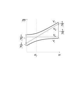
Figure 1: Evolution of the probability

Furthermore the probability of finding the eigenstate in some flavor is given by how close the hyperboles are from the asymptotes. We can interpret FIG. 1 in the classical way. Let us suppose that $N$ electronic neutrinos are produced inside matter, classically there is $N_{1}=NP_{1}$ neutrinos of mass $m_{+}$ and $N_{2}=NP_{2}$ neutrinos of mass $m_{-}$. When they go into the vacuum they are going detected like $N_{e}=P^{0}_{1}N_{1}+P^{0}_{2}N_{2}$ neutrinos of electronic type. Then the survival probability is

$$P_{\nu_{e}\rightarrow\nu_{e}}=\frac{N_{e}}{N}=P^{0}_{1}P_{1}+P^{0}_{2}P_{2}=\frac{1}{2}(1+\cos 2\theta\cos 2\phi).$$ (9)

Actually the neutrinos of mass $m_{+}$ travelling trough matter can be converted into neutrinos of mass $m_{-}$ and vice-versa because a quantum tunneling effect. The number of conversions must be proportional to the difference $N_{1}-N_{2}$, so when they travel in the vacuum there will be $N^{0}_{1}=N_{1}+P(N_{2}-N_{1})$ neutrinos of mass $m_{+}$ and $N^{0}_{2}=N_{2}+P(N_{1}-N_{2})$ neutrinos of mass $m_{-}$, where $P$ is the conversion probability. The number of detected electronic neutrinos is $N_{e}=P^{0}_{1}N^{0}_{1}+P^{0}_{2}N^{0}_{2}$ and the probability for detecting a neutrino electronic is now

$$P_{\nu_{e}\rightarrow\nu_{e}} = P^{0}_{1}P_{1}+P^{0}_{2}P_{2}-P(P_{1}-P_{2})(P^{0}_{1}-P^{0}_{2})$$ (10)

$$= \frac{1}{2}\Big{(}1+(1-2P)\cos 2\theta\cos 2\phi\Big{)}.$$

The conversion probability $P$ is known the Landau-Zener probability

IV Quantum probability

Now let us calculate the Landau-Zener probability from the Schrodinger equation for the neutrino system. Terms proportional to $\sigma_{0}$ in (3) contribute only with an overall phase physically meaningless, so we can drop it. When neutrinos are produced inside matter the mixing angle changes if the density is a function of the position. The angle $\phi$ depends on time while the neutrino traveling in matter. The Schrodinger equation in the matter eigenstates now read

$$ie^{-i\phi\sigma_{2}}\frac{d}{dt}e^{i\phi\sigma_{2}}\nu_{m}=-\Delta\sigma_{3}\nu_{m}$$ (11)

that is

$$i\frac{d}{dt}\nu_{m}=(\dot{\phi}\sigma_{2}-\Delta\sigma_{3})\nu_{m}\equiv H_{e}\nu_{m}.$$ (12)

From (12) $|\dot{\phi}|$ determine the energy transition between the two eigenstates and $\Delta$ give the gap between levels. If

$$\frac{|\dot{\phi}|}{\Delta}\ll 1,$$ (13)

the off-diagonal terms of the effective Hamiltonian $H_{e}$ can be neglected and the system of equations for the eigenstates decouple. This is the condition of adiabaticity. For non-adiabatic limit we can not decouple the neutrino system.

The survival probability for electronic neutrino is

$$P_{\nu_{e}\rightarrow\nu_{e}}(t)=\left|\chi_{\theta}^{\dagger}U(t)\chi_{\phi}\right|^{2}$$ (14)

where $\chi_{\alpha}=(\cos\alpha,\sin\alpha)^{T}$ are the components of the neutrino electronic in the basis of the Hamiltonian eigenstates. $U(t)$ is the temporal evolution operator which satisfy the Schrodinger equation

$$i\frac{d}{dt}U(t)=H_{e}(t)U(t).$$ (15)

Because of unitary $U(t)$ can be written as

$$U(t)=a_{0}(t)\sigma_{0}+i\vec{a}(t)\cdot\vec{\sigma},$$ (16)

where the $a_{i}$ are real and $\sum_{i}a_{i}=1$. The probability (26) in function of this parameters is written asPark

$$P_{\nu_{e}\rightarrow\nu_{e}}(t)=\frac{1}{2}\Big{(}1+\cos{2\theta}\cos{2\phi}(a_{0}^{2}-a_{1}^{2}-a_{2}^{2}+a_{3}^{2})+\cos{2\theta}\sin{2\phi}(a_{1}a_{3}-a_{0}a_{2})$$

$$+\sin{2\theta}\sin{2\phi}(a_{0}^{2}+a_{1}^{2}-a_{2}^{2}-a_{3}^{2})+\sin{2\theta}\cos{2\phi}(a_{1}a_{3}+a_{0}a_{2})\Big{)}.$$ (17)

The $a_{i}$ coefficients can be found solving equation (15) which can be written in a differential form

$$U(t+dt)=\Big{(}1-iH_{e}(t)dt\Big{)}U(t),$$ (18)

with the condition $U(0)=1$. From (18) it is straightforward to find that

$$U(t)=\lim_{N\rightarrow\infty}\prod_{k=0}^{N}\Big{(}1-iH_{e}(kt/N)dt\Big{)}\equiv\Pi\int_{0}^{t}e^{-iH_{e}(t)dt}.$$ (19)

If $[H(t_{1}),H(t_{2})]=0$ for any pair $(t_{1},t_{2})$ trivially

$$\Pi\int_{0}^{t}e^{-iHdt}=e^{-i\int_{0}^{t}H(t)dt}.$$ (20)

If the Hamiltonian does not commute for different times we can do perturbation theory splitting the effective Hamiltonian in a no perturbed and perturbation parts, $H_{e}=H_{0}+H_{1}$, in our case

$$H_{0}=-\Delta\sigma_{3},\;\;H_{1}=\dot{\phi}\sigma_{2}.$$ (21)

Assuming $\langle H_{0}\rangle\gg\langle H_{1}\rangle$ we expand (19) as

$$U(t) = ..\Big{(}e^{-iH_{0}(t-dt)dt}-iH_{1}(t-dt)dt\Big{)}\Big{(}e^{-iH_{0}(t)dt}-iH_{1}(t)dt\Big{)}\Big{(}e^{-iH_{0}(t+dt)dt}-iH_{1}(t+dt)dt\Big{)}..$$

$$= e^{-i\int_{0}^{t}H_{0}dt}$$

$$-i\int_{0}^{t}dt_{1}e^{-i\int_{0}^{t_{1}}H_{0}dt}H_{1}(t_{1})e^{-i\int_{t_{1}}^{t}H_{0}dt}$$

$$-\int_{0}^{t}dt_{2}\int_{0}^{t_{2}}dt_{1}e^{-i\int_{0}^{t_{1}}H_{0}dt}H_{1}(t_{1})e^{-i\int_{t_{1}}^{t_{2}}H_{0}dt}H_{1}(t_{2})e^{-i\int_{t_{2}}^{t}H_{0}dt}.$$

This equation can be graphically represented as

with the Feynman rules

Using (21) the time evolution operator can be expressed as

$$U(t)=\left(\sum_{n=0}^{\infty}(-i\sigma_{2})^{n}\int\prod_{j=1}^{n}dt_{j}\dot{\phi}(t_{j})e^{2i\sigma_{3}\int_{0}^{t_{j}}\Delta dt(-)^{n+j}}\right)$$

$$\times e^{-i\sigma_{3}\int_{0}^{t}\Delta dt}\;\;\;$$ (22)

which can be parametrized as

$$U(t)=(\cos\lambda+i\sigma_{2}\sin\lambda e^{i\beta\sigma_{3}})e^{i\alpha\sigma_{3}},$$ (23)

where $\alpha$ is a monotonous function of time and $\beta$ depends on the time to reach the vacuum. Comparing with (16) we find for the fully averaged probability (17), over the time of production and detection, is

$$\langle P_{\nu_{e}\rightarrow\nu_{e}}\rangle=\frac{1}{2}\Big{(}1+\cos{2\theta}\cos{2\phi}(1-2\sin^{2}\lambda)\Big{)}.$$ (24)

Comparing with (10) we can see that the probability conversion is given by $P=\sin^{2}\lambda$, which is the modulo squared of the $\sigma_{2}$ coefficient in (22), that is

$$P=\left|\sum_{n=0}^{\infty}(-1)^{n}\int\prod_{j=1}^{2n+1}dt_{j}\dot{\phi}(t_{j})e^{-2i\int_{0}^{t_{j}}\Delta dt(-)^{j}}\right|^{2}.$$ (25)

This is an exact expression for the Landau-Zener probability. At lowest order in $\dot{\phi}$, the Landau-Zener probability is

$$P_{LZ}=\left|\int_{0}^{t}dt_{1}\dot{\phi}(t_{1})e^{2i\int_{0}^{t_{1}}\Delta dt}\right|^{2}.$$ (26)

From (5) we obtain

$$\dot{\phi}=\frac{\dot{a}\sin 2\theta}{2(1-2a\cos 2\theta+a^{2})}.$$ (27)

Considering that the main contribution is near the resonance region, $a=\cos 2\theta$ and assuming the neutrinos are produced above this region we can extend the limits of the integral in (26) over all $\tilde{a}=a-\cos 2\theta$,

$$\int_{0}^{t}dt_{1}\dot{\phi}(t_{1})e^{2i\int_{0}^{t_{1}}\Delta dt}\simeq\frac{1}{2}\int_{-\infty}^{\infty}\frac{\sin 2\theta e^{iI(\tilde{a})}}{\tilde{a}^{2}+\sin^{2}2\theta}\,d\tilde{a}$$ (28)

where

$$I(\tilde{a})=2\Delta_{0}\int^{\tilde{a}}\sqrt{\tilde{a}^{2}+\sin^{2}2\theta}\frac{d\tilde{a}}{\dot{a}}.$$ (29)

The integral in (28) has poles in $\tilde{a}=\pm i\sin 2\theta$. This integral is calculated to give

$$P_{LZ}=\frac{\pi^{2}}{4}e^{-2|{\rm Im}I(i\sin 2\theta)|}.$$ (30)

To find (29) we need to know the functional form of $a$. For example assuming $\dot{a}$ constant we have

$$I(i\sin 2\theta)=\frac{2\Delta_{0}}{\dot{a}}\frac{\sin^{2}2\theta}{2}\ln(i\sin 2\theta),$$ (31)

and

$$P_{LZ}=\frac{\pi^{2}}{4}e^{-\gamma\pi/2}$$ (32)

where

$$\gamma=\left.\frac{\Delta}{\dot{\phi}}\right|_{a=\cos\theta}$$ (33)

is the adiabatic parameter. Probabilities for other density distribution can be found in the literature kuo .

In the usual expression for Landau-Zener probability $P_{LZ}\to 1$ when $\gamma\to 0$. It seems that (32) is not correct because at this limit $P_{LZ}\to\pi^{2}/4$ for us. But in this situation the perturbation approach (26) is not valid and we need to take the expression (25).

V Conclusions

In this paper we have reviewed the Landau-Zener probability starting from standard approach and introducing a perturbation method to solve the temporal evolution operator. We found that our expression differs from the standard one by a multiplicative factor $\pi^{2}/4\sim 2.6$ which at the present experimental resolution is irrelevant, but in the interpretation of the neutrino flux from supernova explosion zulu could be very important correction because of the non adiabatic neutrino propagation.

References

(1)
M.Fukugita, T. Yanagida, Physics of neutrinos and aplications to astrophysics,
Springer (2003).
E.Kh. Akhmedov arXiv:hep-ph/0001264 v2 (2000).
Robindra N. Mohapatra, Physics and Astrophysics, Palash B. Pal,
Worl Scientific Notes in Physics, third edition (1998)
C.W.Kim,A.Pevsner, Neutrino in Physics and Astrophysics, harwood academic publishers (1993).
(2)
P. C. de Holanda, Wei Liao, A Yu Smirnov,
Nucl. Phys. B702, 307 (2004).
(3)
A Yu Smirnov,
arXiv: hep-ph/070206v1 (2007).
(4)
C. W. Kim, W. K. Sze and S. Nussinov,
Phys. Rev. D35, 4014 (1987).
(5)
S. M. Bilenky and B. Pontecorvo,
Phys. Rept. 41, 225 (1978).
(6)
Stephen J. Parke,
Phys. Rev. Lett. 57, 1275 (1986).
(7)
T. K. Kuo and James Pantaleone,
Phys. Rev. D39, 1930 (1989).
(8)
E. Nardi and J. I. Zuluaga.
arXiv:astro-ph/0511771v2.