Misaligned spin-orbit in the XO-3 planetary system?

The transiting extrasolar planet XO-3b is remarkable, with a high mass and eccentric orbit. These unusual characteristics make it interesting to test whether its orbital plane is parallel to the equator of its host star, as it is observed for other transiting planets. We performed radial velocity measurements of XO-3 with the SOPHIE spectrograph at the 1.93-m telescope of Haute-Provence Observatory during a planetary transit, and at other orbital phases. This allowed us to observe the Rossiter-McLaughlin effect and, together with a new analysis of the transit light curve, to refine the parameters of the planet. The unusual shape of the radial velocity anomaly during the transit provides a hint for a nearly transverse Rossiter-McLaughlin effect. The sky-projected angle between the planetary orbital axis and the stellar rotation axis should be $\lambda=70^{\circ}\pm 15^{\circ}$ to be compatible with our observations. This suggests that some close-in planets might result from gravitational interaction between planets and/or stars rather than migration due to interaction with the accretion disk. This surprising result requires confirmation by additional observations, especially at lower airmass, to fully exclude the possibility that the signal is due to systematic effects.

1 Introduction

Johns-Krull et al. (jk07 (2008)) announced the detection of XO-3b, an extra-solar planet transiting its F5V parent star with a 3.2-day orbital period. Transiting planets are of particular interest as they allow measurements of parameters including orbital inclination and planet radius, mass and density. Moreover, follow-up observations can also be performed during transits or anti-transits, yielding physical constraints on planetary atmospheres.

Among the forty transiting extra-solar planets known to date, XO-3b is particular as it is among the few on an eccentric orbit, together with HD 147506b (Bakos et al. bakos07 (2007)), HD 17156b (Fischer et al. fischer07 (2007); Barbieri et al. barbieri07 (2007)), and GJ 436b (Butler et al. butler04 (2004); Gillon et al. gillon07 (2007)). XO-3b is also the most massive transiting planet known to date. Most of the sixty known extrasolar planets, with and without transits, with orbital periods shorter than five days have masses below 2 M_Jup; XO-3b is actually one of the rare massive close-in planets. It is just at the limit between low-mass brown dwarfs and massive planets, 13 M_Jup, which is defined by the deuterium burning limit. There was a quite large uncertainty on the planetary parameters of XO-3b and its host star. Indeed, Johns-Krull et al. (jk07 (2008)) presented a spectroscopic analysis favoring large masses and radii ($M_{\mathrm{p}}\simeq 13.25$ M_Jup, $R_{\mathrm{p}}\simeq 1.95$ R_Jup, $M_{\star}\simeq 1.41$ M_⊙, and $R_{\star}\simeq 2.13$ R_⊙), whereas their light curve analysis suggests lower values ($M_{\mathrm{p}}\simeq 12.03$ M_Jup, $R_{\mathrm{p}}\simeq 1.25$ R_Jup, $M_{\star}\simeq 1.24$ M_⊙, and $R_{\star}\simeq 1.48$ R_⊙) [see however Sect. 5 and Winn et al. (2008a )].

The fast rotating star XO-3 ($V\sin I=18.5$ km s^-1; Johns-Krull et al. jk07 (2008)) is a favorable object for Rossiter-McLaughlin effect observations. This effect (Rossiter rossiter24 (1924); McLaughlin mclaughlin24 (1924)) occurs when an object transits in front of a rotating star, causing a distortion of the stellar lines profile, and thus an apparent anomaly in the measured radial velocity of the star. The shape of the disturbed radial velocity curve allows one to determine whether the planet is orbiting in the same direction as its host star is rotating, and more generally to measure the sky-projected angle between the planetary orbital axis and the stellar rotation axis, usually noted $\lambda$ (see, e.g., Ohta et al. ohta05 (2005); Giménez 2006a ; Gaudi & Winn gaudi07 (2007)). A stellar spin axis not aligned with the orbital angular momentum of a planet ($\lambda\neq 0^{\circ}$) could reflect processes in the planet formation and migration, or interactions with perturbing bodies (see, e.g., Malmberg et al. malmberg07 (2007), Chatterjee et al. chatterjee07 (2007), Nagasawa et al. nagasawa08 (2008)). Solar System asteroids are examples of objects whose orbital axes can be misaligned from the Sun spin axis by over $30^{\circ}$.

Up to now, spectroscopic transits have been detected for eight exoplanets: HD 209458b (Queloz et al. queloz00 (2000)), HD 189733b (Winn et al. winn06 (2006)), HD 149026b (Wolf et al. wolf07 (2007)), TrES-1 (Narita et al. narita07 (2007)), HD 147506b (Winn et al. winn07 (2007); Loeillet et al. loeillet07 (2008)), HD 17156b (Narita et al. narita08 (2008)), CoRoT-Exo-2b (Bouchy et al. bouchy08 (2008)) and TrES-2 (Winn et al. 2008b ). For all of these targets the stellar rotation is prograde relative to the planet orbit, and the sky-projected $\lambda$ angle is close to zero for most of them. So the axes of the stellar spins are probably parallel to the orbital axes, as expected for planets that formed in a protoplanetary disc far from the star and that later migrated closer-in. Three systems have error bars on the $\lambda$ angle that do not include $0^{\circ}$: TrES-1 ($\lambda=30^{\circ}\pm 21^{\circ}$), CoRoT-Exo-2b ($\lambda=7.2\pm 4.5^{\circ}$) and HD 17156b ($\lambda=62^{\circ}\pm 25^{\circ}$). However, those cases have the largest error bars on $\lambda$, and no firm detection of misalignment has yet been claimed. Barbieri et al. (barbieri08 (2008)) recently presented new radial velocity measurements of HD 17156 secured during a transit, which agree with a spin-orbit alignment.

Approximate spin-orbit alignment therefore seems typical for exoplanets, as it is for planets in the Solar System. The unusual parameters of XO-3b make a test of whether it agrees with this apparent behavior interesting. We present here new measurements of XO-3 radial velocity performed during a transit and at other orbital phases. These data refine the orbital parameters and provide a hint of detection for a transverse Rossiter-McLaughlin effect, i.e.  a $\lambda$ angle possibly near $90^{\circ}$. We also present a revised analysis of the transit light curve.

2 Observations

We observed the host star XO-3 (GSC 03727-01064, $m_{V}=9.91$) with the SOPHIE instrument at the 1.93-m telescope of Haute-Provence Observatory, France. SOPHIE is a cross-dispersed, environmentally stabilized echelle spectrograph dedicated to high-precision radial velocity measurements (Bouchy et al. bouchy06 (2006)). We used the high-resolution mode (resolution power $R=75,000$) of the spectrograph, and the fast-read-out-time mode of the $4096\times 2048$ 15-$\mu$m-pixel CCD detector. The two optical-fiber circular apertures were used; the first one was centered on the target, and the second one was on the sky to simultaneously measure its background. This second aperture, 2’ away from the first one, was used to estimate the spectral pollution due to the moonlight, which can be quite significant in these 3”-wide apertures (see Sect. 3).

We acquired 36 spectra of XO-3 during the night of January 28th, 2008 (barycentric Julian date BJD$\;=2\,454\,494.5$), where a full coverage of the planetary transit was observed. Another 19 spectra were acquired at other orbital phases during the following two months. Table 1 summaries the 55 spectra finally acquired.

Table 1: Radial velocities of XO-3 measured with SOPHIE.

BJD	RV	$\pm$$1\,\sigma$	exp. time	S/N p. pix.
-2 400 000	(km s-1)	(km s-1)	(sec)	(at 550 nm)
Planetary transit:
54494.4461	-11.298	0.020	600	54
54494.4526	-11.300	0.026	403	42
54494.4578	-11.345	0.027	373	40
54494.4625	-11.379	0.027	370	40
54494.4675	-11.390	0.028	370	39
54494.4721	-11.354	0.028	370	39
54494.4767	-11.460	0.029	370	38
54494.4813	-11.448	0.028	381	39
54494.4861	-11.419	0.027	380	40
54494.4913	-11.411	0.027	380	40
54494.4960	-11.457	0.028	380	39
54494.5007	-11.463	0.028	380	39
54494.5054	-11.549	0.028	380	39
54494.5101	-11.482	0.028	380	40
54494.5152	-11.589	0.028	380	39
54494.5202	-11.652	0.028	434	39
54494.5254	-11.611	0.027	403	40
54494.5303	-11.679	0.027	392	40
54494.5352	-11.691	0.036	395	40
54494.5413	-11.667	0.035	509	43
54494.5474	-11.782	0.034	500	44
54494.5535	-11.700	0.034	500	42
54494.5599	-11.649	0.035	554	44
54494.5665	-11.785	0.034	531	44
54494.5738	-11.811	0.036	530	44
54494.5806	-11.783	0.033	602	45
54494.5880	-11.867	0.033	622	44
54494.5957	-11.767	0.033	653	45
54494.6036	-11.785	0.035	650	46
54494.6123	-11.740	0.034	682	45
54494.6210	-11.783	0.035	775	45
54494.6305	-11.880	0.033	801	45
54494.6407	-11.843	0.034	906	44
54494.6532	-11.920	0.036	964	42
54494.6668	-11.964	0.037	1321	43
54494.6822	-11.913	0.049	1300	38
Other orbital phases:
54496.2649	-12.723	0.050	1202	22
54497.2609	-10.156	0.029	655	37
54499.2765	-13.006	0.030	1003	36
54501.2926	-12.433	0.031	775	34
54501.4628	-12.756	0.033	775	34
54502.2730	-13.068	0.024	614	44
54503.2614	-10.936	0.030	907	35
54503.4700	-10.182	0.040	1806	29
54504.4321	-12.398	0.028	645	39
54505.2889	-13.132	0.023	635	46
54506.2904	-11.593	0.025	755	43
54511.4534	-13.041	0.038	600	48
54512.4618	-12.246	0.036	600	41
54513.3091	-10.360	0.052	600	48
54516.3517	-10.176	0.046	600	39
54516.4540	-10.267	0.071	802	32
54551.3044	-10.316	0.032	1274	37
54553.3002	-13.135	0.033	999	36
54554.3114	-11.004	0.019	999	57

The exposure times range from 6 to 30 minutes in order to reach as constant the signal-to-noise ratio as possible. Indeed, SOPHIE radial velocity measurements are currently affected by a systematic effect at low signal-to-noise ratio, which is probably due to CCD charge transfer inefficiency that increases at low flux level. A constant signal-to-noise ratio through a sequence of observations reduces this uncertainty. The different exposure times needed to reach similar signal-to-noise ratios reflect the variable throughputs obtained, due to various atmospheric conditions (seeing, thin clouds, atmospheric dispersion). The sky was clear on the night whom the XO-3b transit was observed, but the airmass ranged from 1.2 to 3.1 during this $\sim$6-hour observation sequence; the exposure times therefore increased during the transit observation. They remain short enough to provide a good time sampling (20 measurements during the $\sim$3 hours of the transit). The 19 measurements outside the transit night were performed at airmasses better than 1.4 but with conditions varying from photometric to cloudy.

Exposures of a thorium-argon lamp were performed every 2-3 hours during each observing night. Over 2-3 hours, the observed drifts were typically $\sim 3$ m s^-1, which is thus the accuracy of the wavelength calibration of our XO-3 SOPHIE spectra; this is good enough for the expected signal. We did not use simultaneous calibration to keep the second aperture available for sky background estimation. During the night of January 28th, 2008, we performed a thorium-argon exposure before the transit and another one after the sequence, about six hours later. The measured drift was particularly low this night, 1 m s^-1  in six hours, which makes us confident the wavelength calibration did not unexpectedly drift during the observation of the XO-3b transit.

3 Data reduction

We extracted the spectra from the detector images and measured the radial velocities using the SOPHIE pipeline. Following the techniques described by Baranne et al. (baranne96 (1996)) and Pepe et al. (pepe02 (2002)), the radial velocities were obtained from a weighted cross-correlation of the spectra with a numerical mask. We used a standard G2 mask constructed from the Sun spectrum atlas including more than 3500 lines, which is well adapted to the F5V star XO-3. We eliminated the first eight spectral orders of the 39 available ones from the cross-correlation; these blue orders are particularly noisy, especially for the spectra obtained at the end of the transit, when the airmass was high. The resulting cross-correlation functions (CCFs) were fitted by Gaussians to get the radial velocities, as well as the width of the CCFs and their contrast with respect to the continuum. The uncertainty on the radial velocity was computed from the width and contrast of the CCF and the signal-to-noise ratio, using the empirical relation detailed by Bouchy et al. (bouchy05 (2005)) and Collier Cameron et al. (cameron07 (2007)). It was typically around 25 m s^-1 during the night of the transit, and between 20 and 45 m s^-1  the remaining nights. The large $V\sin I$ of this rotating stars makes the uncertainty slightly larger than what is usually obtained for such signal-to-noise ratios with SOPHIE.

Some measurements were contaminated by the sky background, including mainly the moonlight. As the G2 mask matches the XO-3 spectrum as well as the Sun spectrum reflected by the Moon and the Earth atmosphere, the moonlight contamination can distort the shape of the CCF and thus shift the measured radial velocity. During our observations, the 29-km s^-1 wide (FWHM) CCF of XO-3 is at radial velocities between $-13$ and $-10$ km s^-1, whereas the moonlight was centered near the barycentric Earth radial velocity, between $-23$ and $-20$ km s^-1. Thus moonlight contamination tends to blueshift the measured radial velocities. Following the method described in Pollacco et al. (pollacco08 (2008)) and Barge et al. (barge08 (2008)), we estimated the Moon contamination thanks to the second aperture, targeted on the sky, and then subtracted the sky CCF from the star CCF (after scaling by the throughput of the two fibers). Five exposures with too strong contamination were not used. We estimated the accuracy of this correction on one hand by correcting uncontaminated spectra, and on the other hand by correcting uncontaminated spectra on which we have added moonlight contaminations. Comparisons of the corrected velocities to the uncontaminated ones show that the method works well up to $\sim 500$ m s^-1 shifts, with an uncertainty of 1/9 of the correction to which a minimum uncertainty of 25 m s^-1 is quadratically added.

The second half of the transit night measurements was contaminated by moonlight, with sky CCFs contrasted between 2 and 5 % of the continuum, whereas the XO-3 CCF has a contrast of 8 %. This implied sky corrections $<150$ m s^-1 (except for the very last exposure where it was $\sim 300$ m s^-1), with uncertainties in the range 25-30 m s^-1 (40 m s^-1 for the last exposure). Five exposures obtained later at different phases were contaminated by the moonlight; corrections of 100 to 500 m s^-1 were computed, with uncertainties in the range 30-60 m s^-1.

The final radial velocities are given in Table 1 and displayed in Figs. 1 and 2. The error bars are the quadratic sums of the different error sources (photon noise, wavelength calibration and drift, moonlight correction).

Figure 1: Top: Radial velocity measurements of XO-3 as a function of time, and Keplerian fit to the data (without transit). Only the 23 measurements used for the fit are displayed. The orbital parameters corresponding to this fit are reported in Table 2. Bottom: Residuals of the fit with 1-$\sigma$  error bars.

4 Determination of the planetary system parameters

4.1 Refined orbit

The radial velocities measurements presented by Johns-Krull et al. (jk07 (2008)) have a typical accuracy of $\sim 160$ m s^-1. Those secured with SOPHIE are about five times more accurate, so they allow for a refinement of the original parameters of the system. We made a Keplerian fit of the first four SOPHIE measurements performed during the transit night and those performed afterwards, at other phases, first using the orbital period from Johns-Krull et al. (jk07 (2008)). For the refinement of the orbit we did not use most of the data secured during the night of January 28th, 2008, in order to remain free from alteration due to transit anomalies and possible systematic effects due to large-airmass observations.

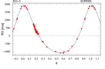
Figure 2: Phase-folded radial velocity measurements of XO-3 (corrected from the velocity $V_{r}=-12.045\,$km s^-1) as a function of the orbital phase, and Keplerian fit to the data. Orbital parameters corresponding to this fit are reported in Table 2. For display purpose, all the measurements performed during the transit night are plotted here. However, only the first four measurements of the transit night are used for the orbit fit, together with 19 measurements secured at other orbital phases (see § 4.1). Figs. 5 and 7 display a magnification on the transit night measurements.

The standard deviation of the residuals to the fit is $\sigma(O-C)=29$ m s^-1, implying a $\chi^{2}$  of 15.3, which is acceptable according the low degrees of freedom, $\nu=18$. The 29 m s^-1 dispersion of the measurements around the fit is similar to the errors on the individual radial velocity measurements; these estimated error bars thus are approximatively correct. The fits are plotted in Figs. 1 and 2; the derived orbital parameters are reported in Table 2, together with error bars, which were computed from $\chi^{2}$  variations and Monte Carlo experiments. They agree with the Johns-Krull et al. (jk07 (2008)) parameters but the error bars are reduced by factors of three to six. The largest difference is on the eccentricity, which we found 1.6$\,\sigma$ larger than Johns-Krull et al. (jk07 (2008)). The residuals, plotted as a function of time in the bottom panel of Fig. 1, do not show any trend that might suggest the presence of another companion in the system over two months.

Table 2: Fitted orbit and planetary parameters for XO-3b.

Parameters	Values and 1-$\sigma$ error bars	Unit
$V_{r}$	$-12.045\pm 0.006$	km s-1
$P$	$3.19161\pm 0.00014$	days
$e$	$0.287\pm 0.005$
$\omega$	$-11.3\pm 1.5$	∘
$K$	$1.503\pm 0.010$	km s-1
$T_{0}$ (periastron)	$2\,454\,493.944\pm 0.009$	BJD
$\sigma(O-C)$	29	m s-1
reduced $\chi^{2}$	0.85
$N$	23
$t_{c}$ (transit)	$2\,454\,494.549\pm 0.014$	BJD
$M_{\star}$	$1.3\pm 0.2$	M⊙
$R_{\star}$	$1.6\pm 0.2$	R⊙
$M_{\textrm{p}}\sin i$	$12.4\pm 1.9$†	MJup
$i$	$82.5\pm 1.5$	∘
$M_{\textrm{p}}$	$12.5\pm 1.9$†	MJup
$R_{\textrm{p}}$	$1.5\pm 0.2$	RJup
$\lambda$	$70\pm 15$	∘
$\dagger$: using $M_{\star}=1.3\pm 0.2$ M⊙

Fitted alone, the 23 SOPHIE measurements have too short time span (60 days) to measure the period more accurately than Johns-Krull et al. (jk07 (2008))  from photometric observations of twenty transits. A 1.5-year time span is obtained when the SOPHIE measurements are fitted together with the radial velocities measured by Johns-Krull et al. (jk07 (2008)) using the telescopes Harlan J. Smith (HJS) and Hobby-Eberly (HET). This longer time span allows a more accurate period measurement. We obtained $P=3.19168\pm 0.00015$ days from the fit using the three datasets, in agreement with the photometric one, and with a similar uncertainty. The final period reported in Table 2 ($P=3.19161\pm 0.00014$ days) reflect these two measurements and is used for the fits plotted in Figs. 1 and 2. Adding HJS and HET data does not significantly change the other orbital parameters nor their uncertainties. For the global fit using the radial velocities from the three instruments, we did not use the last HET measurement, performed during a transit (see Sect. 6).

The Keplerian fit of the new SOPHIE radial velocity measurements also improves the transit ephemeris, as the photometric transits reported by Johns-Krull et al. (jk07 (2008)) were secured between December 2003 and March 2007, one hundred or more XO-3b revolutions before the January 28th, 2008 transit. The mid-point of this transit predicted from the Keplerian fit of the SOPHIE radial velocity measurements is $t_{c}=2\,454\,494.549\pm 0.014$ (BJD), i.e. just a few minutes earlier than the prediction from Johns-Krull et al. (jk07 (2008)). The uncertainty on this transit mid-point is $\pm 20$ minutes (or $\pm 0.004$ in orbital phase).

In order to reduce this uncertainty, we observed a recent photometric transit of XO-3b with a 30-cm telescope at the Teide Observatory, Tenerife, Spain, on February 29th, 2008 (Fig. 3). Weather conditions were poor and we therefore analyzed the transit with a fixed model based on the algorithm of Giménez (2006b ). The fixed parameters were the ratio between the radii of the star and of the planet $k=0.0928$, the sum of the projected radii $rr=0.2275$, the inclination $i=79.3^{\circ}$, and the eccentricity $e=0.26$. We then scanned different mid-transit times and found $t_{c}=2\,454\,526.4668\pm 0.0026$ (BJD) from $\chi^{2}$  variations. This reflects photon noise only; fluctuations due to poor weather may introduce additional uncertainties. By taking into account for the uncertainty on the orbital period, this translates into $t_{c}=2\,454\,494.5507\pm 0.0030$ (BJD) for the spectroscopic transit that we observed with SOPHIE on January 28th, 2008, i.e. ten revolutions earlier. That is just two minutes after the above prediction from SOPHIE ephemeris, and the uncertainty on this transit mid-point is $\pm 4.3$ minutes (or $\pm 0.0009$ in orbital phase).

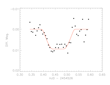
Figure 3: Light curve of XO-3 observed at the Teide Observatory, Tenerife, during the transit of February 29th, 2008. The transit fit (solid line) provides $t_{c}=2\,454\,526.4668\pm 0.0026\equiv 2\,454\,494.5507\pm 0.0030$ (BJD).

4.2 Transit light curve fit revisited

Johns-Krull et al. (jk07 (2008)) point out that the host star radius obtained from the spectroscopic parameters (temperature, gravity, metallicity) combined with stellar evolution models, $R_{\star}\simeq 2.13$ R_⊙, is incompatible with the value obtained from the shape of the transit light curve, namely $R_{\star}\simeq 1.48$ R_⊙. Indeed, a large stellar radius implies a large planetary radius (to account for the depth of the transit) and a large inclination angle (to account for the duration of the transit), but the time from the first to the second contacts (ingress) and third to fourth contacts (egress) predicted for such an inclination are too long when compared to the observed transit light curve (see the upper panel of Fig. 9 in Johns-Krull et al. jk07 (2008)). Formal uncertainties on the stellar spectroscopic parameters and the photometric measurements are insufficient to account for the mismatch. Since there can be only one value of the real stellar radius, this must be due to systematic uncertainties on the spectroscopic parameters, or the parameter derivation from the photometric data, or both. We revisit these analyses below, using the photometric data from Johns-Krull et al. (jk07 (2008)) and the parameters of the Keplerian orbit obtained in § 4.1 from the SOPHIE radial velocity measurements.

Regarding the spectroscopic parameters, the formal uncertainties stated by Johns-Krull et al. (jk07 (2008)), e.g. 0.06 dex for the gravity $\log g$ or 0.03 dex for the metallicity $Z$, are particularly small. Since these are used in combination with stellar evolution models, even if the actual uncertainties on the observations are small, systematic uncertainties are known to be present in the models themselves. Also, precise gravity measurements are difficult to obtain from stellar spectra. We therefore set a floor level of effective uncertainties in the confrontation with stellar evolution models of 100 $K$ in temperature, of 0.1 dex in $\log g$, or 0.1 dex in $Z$ (see e.g. discussion in Santos et al. santos04 (2004) and Pont & Eyer pont04 (2004)).

Regarding the photometric data, we estimated the uncertainties including systematics effects with “segmented bootstrap” analysis (Jenkins et al. jenkins02 (2002); Moutou et al. moutou04 (2004)). According to Pont et al. (pont06 (2006)), correlated noise usually dominates the total parameter error budget for ground-based transit light curves. The segmented bootstrap consist of repeating the fit on realizations of the data with individual nights selected at random. The photometric follow-up for XO-3 by Johns-Krull et al. (jk07 (2008)) consists of ten individual nights. Since the sequencing of the data within each night is preserved, this method provide error estimates that takes into account the actual correlated noise in the data. We find much larger uncertainties on the impact parameter than the photon-noise uncertainties. This is corroborated by the discussion in Bakos et al. (bakos06 (2006)) of the case of HD 189733. With a much deeper transits and a similar number of high-precision photometry transits covered from several observatories, they found that the determination of the stellar radius from the photometric data produced an error of $\sim 15$ %, consistent with the discussion in Pont et al. (pont06 (2006)).

Figure 4: Posterior probability distribution function for the stellar radius of XO-3 obtained from Bayesian approach. Dashed line: Using only the constraints from the light curves of Johns-Krull et al. (jk07 (2008)) and the parameters of the Keplerian orbit (§ 4.1). Dotted line: Using only the constraints from the spectroscopic parameters. Solid line: Using all these constraints together.

To estimate the probability distribution of the radius of XO-3 given the available photometric and spectroscopic observations, and the a priori assumption that the star is located near theoretical stellar evolution tracks, we use a Bayesian approach. As discussed in Pont & Eyer (pont04 (2004)), such approach is needed for realistic parameter estimates when the uncertainties are not small compared to the total parameter space and the relation between parameters and observable quantities are highly non-linear. We thus calculate the posterior probability distribution of the stellar radius $R_{\star}$, using Bayes’ theorem with stellar evolution models and prior probability distributions suitable for a Solar-Neighbourhood magnitude-limited sample, as discussed in Pont & Eyer (pont04 (2004)) in the context of the Geneva-Copenhaguen survey.

The posterior probability distribution for the stellar radius is calculated according to Bayes’ theorem:

$${\cal P}(R_{\star}|PS)=\int{\cal P}(P|R_{\star}){\cal P}(S|R_{\star}){\cal P}(R_{\star})$$

where $R_{\star}$ is the stellar radius, $P$ the photometric observations and $S$ the spectroscopic observations. The first two terms on the right are the likelihood of the photometric and spectroscopic observations, $\exp(-1/2\chi^{2})$, the last term is the a priori distribution of $R_{\star}$. The integral covers the mass, age and metallicity parameters. The stellar evolution models provide the function $R_{\star}=R_{\star}(M_{\star},Z,\mathrm{age})$. For more detailed explanations of the method see Pont & Eyer (pont04 (2004)).

Fig. 4 displays the posterior probability distribution function for the stellar radius obtained from this Bayesian approach given the spectroscopic and photometric data from Johns-Krull et al. (jk07 (2008)), the stellar evolution models from Girardi et al. (girardi02 (2002)), and the orbit parameters determined from the Keplerian fit of the SOPHIE radial velocity measurements (§ 4.1). The probability distribution function for the radius of XO-3 is centered near $R_{\star}\simeq 1.5$ R_⊙, but extends with non-negligible density from 1.3 to 2.0 R_⊙. It is well described by $R_{\star}=1.6\pm 0.2$ R_⊙. The corresponding masses are $M_{\star}=1.3\pm 0.2$ M_⊙. This is a quantification of our “best guess” from the present observational data and prior knowledge about field stars. These parameters are reported in Table 2.

4.3 Transverse Rossiter-McLaughlin effect?

The radial velocities of XO-3 measured with SOPHIE during the transit of January 28th, 2008 are plotted in Fig. 5. Surprisingly, they do not show the ordinary anomaly seen in case of prograde transit, i.e. a red-shifted radial velocity in the first half of the transit, then blue-shifted in its second half. During the full transit of XO-3b, the radial velocity is blue-shifted from the Keplerian curve, by about 100 m s^-1. Such shape is expected for a transverse Rossiter-McLaughlin effect, i.e. when the $\lambda$ misalignment angle is near $90^{\circ}$ so the the planet crosses the stellar disk nearly perpendicularly to the equator of the star. This is apparently the case for XO-3b, whose transit seems to only hide some red-shifted velocity components, i.e. a part of the star rotating away from the observer. A schematic view of the XO-3 system with a transverse transit is shown in Fig. 6.

We overplot in Fig. 5 models of Rossiter-McLaughlin effects for XO-3b, for $\lambda=0^{\circ}$ (upper panel) and $\lambda=90^{\circ}$ (lower panel). Following Loeillet et al. (loeillet07 (2008)) and Bouchy et al. (bouchy08 (2008)), we used the analytical Ohta et al. (ohta05 (2005)) description of the Rossiter-McLaughlin anomaly. We adopted the orbital parameters of Table 2, a projected stellar rotation velocity $V\sin I$ of 18.5 km s^-1, and a linear limb-darkening coefficient $\epsilon=0.69$ from Claret (claret04 (2004)), for $T_{\mathrm{eff}}=6250$ K and $\log g=4.0$ dex. The transit was centered on the $t_{c}$ time determined above from the February 29th, 2008 photometric transit. To take into account for the large uncertainty in the masses and radii of the star and its planet derived from spectroscopic and light curve analyses (§ 1 and § 4.2), we plot the models using two extreme sets of parameters over the SOPHIE radial velocities in each panel of Fig. 5: the solid line is the Rossiter-McLaughlin model with large masses and radii as favored from spectroscopic analyses, and the dashed line is the Rossiter-McLaughlin model with smaller masses and radii as favored by the light curve analysis. The dotted line is, for comparison, the Keplerian curve without Rossiter-McLaughlin effect.

Table 3 summaries the parameters used for the different models and the quantitative estimations of the quality of the fits. Note that the inclination used by Johns-Krull et al. (jk07 (2008)) for large masses and radii, namely $i=79.32^{\circ}$, produces slightly too long transits duration when used together with our refined orbit. We used $i=78.6^{\circ}$ in that case, which remains within the $\pm 1.36^{\circ}$ error bar obtained on $i$ by Johns-Krull et al. (jk07 (2008)). Models with $\lambda=0^{\circ}$, or without Rossiter-McLaughlin effect detection, produce poor fits, with high $\chi^{2}$ values and radial velocity dispersions of 60 to 75 m s^-1. This is significantly higher than the expected uncertainties on radial velocity measurements, around 33 m s^-1 (see Table 1) and the residuals of the Keplerian fit presented in § 4.1, $\sigma(O-C)=29$ m s^-1. Thus, our SOPHIE  data seem to exclude such ordinary solutions.

The models with $\lambda=90^{\circ}$ produces lower $\chi^{2}$, with velocity dispersions of 42 or 44 m s^-1. The lower panel of Fig. 5 shows that transverse transits produce better fits of the data, centered on the expected mid-transit and with the adequate duration and depth. One should also note that the SOPHIE measurements performed just after the transit (orbital phases from 0.21 to 0.23) are well described by the Keplerian orbit model (see Figs. 2 and 5). We recall that these points were not used to determine the Keplerian orbit (§ 4.1); the orbital parameters were determined using only the first four measurements of the January 28th, 2008 night (filled squares in Fig. 5), together with the measurements secured on other nights. The good match of the data with the $\lambda=90^{\circ}$ models argues for a transverse transit. This possible detection is independent of the set of stellar parameters adopted in Table 3; both produce similar fits with $\lambda=90^{\circ}$. The $\chi^{2}$ is slightly better in the case of large masses and radii but this does not seem to be significant according the noise level.

Figure 5: Rossiter-McLaughlin effect models. Top: $\lambda=0^{\circ}$ (spin-orbit alignment). Bottom: $\lambda=90^{\circ}$ (transverse transit). On both panels, the squares (open and filled) are the SOPHIE radial-velocity measurements of XO-3 with 1-$\sigma$  error bars as a function of the orbital phase. Only the first four measurements (filled squares) are used for the Keplerian fit (together with 19 measurements at other orbital phases; see § 4.1). The dotted line is the Keplerian fit without Rossiter-McLaughlin effect. The two other lines show Rossiter-McLaughlin models with $i=78.6^{\circ}$ and $a/R_{\star}=4.8$ (solid line) and $i=84.9^{\circ}$ and $a/R_{\star}=7.2$ (dashed line). The summary of these parameters is in Table 3.

Table 3: Chosen parameters for the Rossiter-McLaughlin effect models plotted in Fig. 5 (see text).

$a/R_{\star}$	$a$	$M_{\star}$	$R_{\star}$	$M_{\mathrm{p}}$	$R_{\mathrm{p}}$	$i$	$\lambda$	$\sigma$	$\chi^{2}$
	UA	M⊙	R⊙	MJup	RJup	∘	∘	m s-1
4.8	0.048	1.4	2.1	13.7	2.0	78.6	0	61	196
4.8	0.048	1.4	2.1	13.7	2.0	78.6	90	42	63
7.2	0.045	1.2	1.3	12.3	1.2	84.9	0	74	291
7.2	0.045	1.2	1.3	12.3	1.2	84.9	90	44	79
without transit:								59	169

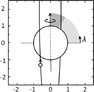
Figure 6: Schematic view of the XO-3 system with transverse transit, as seen from the Earth. The stellar spin axis is shown, as well as the planet orbit and the $\lambda$ misalignment angle. The scale is in stellar radii. The limit between soft and strong grey on the $\lambda$-scale represents the favored value from our observations ($\lambda=70^{\circ}$, see Sect. 5).

The $\sim 40$ m s^-1 dispersion of the data from these transverse models remains slightly above the computed uncertainties on radial velocity measurements. This suggests that some extra uncertainties might be present and not taken into account in the error budget. This make us considering this observation as a hint of detection for a spin-orbit misalignment.

An explanation for this too large dispersion could be the high atmospheric refraction. Indeed, as seen in Sect. 2, the end of the transit was observed at large airmass. This could introduce biases in the radial velocity measurements that are difficult to quantify. This agrees with the increasing dispersion of the data from these transverse models, which is in the range $30-35$ m s^-1 in the first half of the transit, then in the range $40-45$ m s^-1 in the second half.

The larger dispersion might also be partly explained as the expected errors are increasing in the second part of the transit because of moonlight correction (see § 3). In addition, it is possible that the planet was crossing the stellar disk above a spot; this could cause extra radial velocity variations (jitter), as the anomaly that is visible near the phase 0.19. Stellar H and K Ca II lines do not show core emissions, but they are less deep than other F5 stars. This implies $\log R^{\prime}_{\mathrm{HK}}=-4.6\pm 0.2$, and we can not exclude XO-3 presents stellar activity, including spots.

5 A small radius for XO-3b

Shortly after the submission of this paper, photometry of 13 transits of XO-3b were released by Winn et al. (2008a ). These new observations strongly favors the smaller values for XO-3 and XO-3b radii and masses. The parameters reported by Winn et al. (2008a ) agree with the ones presented here (Table 2); this strengthen the Bayesian approach we used in §4.2. Timing parameters (as $P$ or $T_{0}$) from Winn et al. (2008a ) are more accurate thanks to their high-quality transit photometry, whereas orbital parameters (as $e$, $\omega$ or $K$) are more accurate in the present study due to the high-quality radial velocity measurements with SOPHIE.

The small $R_{\mathrm{p}}$ value excludes a grazing transit for XO-3b, and the corresponding models plotted in solid lines in Fig. 5; the Rossiter-McLaughlin anomaly should thus be large and detectable, with an amplitude near the order of magnitude $(V\sin I)(R_{\mathrm{p}}/R_{\star})^{2}\simeq 150$ m s^-1  (Winn et al. 2008a ). We fitted the SOPHIE data using the updated parameters from Winn et al. (2008a ), in particular $R_{\mathrm{p}}=1.217$ R_Jup, $a/R_{\star}=7.07$ and $i=84.20^{\circ}$. According $\chi^{2}$ variations, the range of $\lambda$ compatible with our observations is $70^{\circ}\pm 15^{\circ}$. The lowest $\chi^{2}$ is $\sim 64$, implying a 42 m s^-1 velocity dispersions around the model. The best fit with these parameters is plotted in Fig. 7. The residuals are plotted in Fig. 8 in three cases: without transits, with spin-orbit alignment, and with $\lambda=70^{\circ}$. Among them, the last case is clearly favored by our data when the parameters from Winn et al. (2008a ) are adopted.

Figure 7: Rossiter-McLaughlin effect models with $\lambda=70^{\circ}$ and the small $R_{\mathrm{p}}$ value reported by Winn et al. (2008a ). The squares (open and filled) are the SOPHIE radial-velocity measurements of XO-3 with 1-$\sigma$  error bars as a function of the orbital phase. Only the first four measurements (filled squares) are used for the Keplerian fit (together with 19 measurements at other orbital phases; see § 4.1). The dotted line is the Keplerian fit without Rossiter-McLaughlin effcet. The solid and dotted lines are the models with and without Rossiter-McLaughlin effect.

Figure 8: Residuals of the Rossiter-McLaughlin effect fits. Top: Without transit. Middle: $\lambda=0^{\circ}$ (spin-orbit alignment). Bottom: $\lambda=70^{\circ}$. The squares (open and filled) are the SOPHIE radial-velocity measurements of XO-3 with 1-$\sigma$  error bars as a function of the orbital phase. Only the first four measurements (filled squares) are used for the Keplerian fit (together with 19 measurements at other orbital phases; see § 4.1). The vertical, dashed line shows the center of the transit.

6 Conclusion and discussion

Table 2 summarizes the star, planet and orbit parameters of the XO-3 system that we obtained from our analyses. The radial velocity measurements that we performed with SOPHIE during a planetary transit suggest that the spin axis of the star XO-3 could be nearly perpendicular to the orbital angular momentum of its planet XO-3b ($\lambda=70^{\circ}\pm 15^{\circ}$). We note that one Johns-Krull et al. (jk07 (2008)) HET measurement was obtained near a mid-transit of XO-3b. This radial velocity is blue-shifted by ($260\pm 194$) m s^-1 from the Keplerian curve, in agreement with the possible transverse Rossiter-McLaughlin effect we report here, though with a modest significance.

The SOPHIE observation remains noisy, showing more dispersion around the fit during the transit than at other phases. We consider this result as a tentative detection of transverse transit rather than a firm detection. Indeed, the end of the transit was observed at large airmasses, which could possibly biases the radial velocity measurements. Our fits favor a transverse transit, but one can not totally exclude a systematic error that would mimic by chance the shape of a transverse transit. This would imply that the radial velocities measured during the end of the transit night, at large airmasses, would be off by about 100 m s^-1, i.e. three to four times the expected errors. Other spectroscopic transits of XO-3b should thus be observed. They will allow the transverse Rossiter-McLaughlin effect to be confirmed or not, and to better quantify its parameters, such as the value of the misalignment angle $\lambda$.

Narita et al. (narita08 (2008)) estimate that the timescale for spin-orbit alignment through tidal dissipation is longer than thousand Gyrs. This timescale is uncertain, but much longer than the timescale for orbit circularization, which itself is longer than the age of XO-3, estimated in the range $2.4-3.1$ Gyrs (Johns-Krull et al. jk07 (2008)); there are thus no obvious reasons to exclude an eccentric, transverse system. A strong spin-orbit misalignment would favor of formation scenarii that invokes planet-planet scattering (Ford & Rasio ford06 (2006)) or planet-star interaction in a binary system (Takeda et al. takeda08 (2008)) rather than inward migration due to interaction with the accretion disk. This suggests in turn that some close-in planets might result from gravitational interaction between planets and/or stars. Chatterjee et al. (chatterjee07 (2007)) and Nagasawa et al. (nagasawa08 (2008)) have recently shown that scattering with at least three large planets can account for hot Jupiters and predicts high spin-orbit inclinations (see also Malmberg et al. malmberg07 (2007)). On another hand, XO-3b is an object close to the higher end of planetary masses. As discussed for instance by Ribas & Miralda-Escudé (ribas07 (2007)), there are some indications that these objects be low-mass brown dwarfs, formed by gas cloud fragmentation rather than core accretion; so that XO-3b may not necessarily constrain planet formation scenario.

Finally, pseudo-synchronization might be questioned in the case of the massive XO-3b ($M_{\mathrm{XO-3}}\simeq 100\times M_{\mathrm{XO-3b}}$), which moves on an eccentric orbit with a periastron particularly near its host star. Tidal frictions might be high enough to tune the stellar rotation velocity close to the velocity of its companion on its orbit at the periastron (Zahn zahn77 (1977)). The expected pseudo-synchronized stellar rotation is given by $V_{\mathrm{rot}}=V_{\mathrm{p}}\times\frac{R_{\star}}{a(1-e)}$, where $V_{\mathrm{p}}=2\pi\frac{a}{P}\sqrt{\frac{1+e}{1-e}}$ is the planet velocity at the periastron. For the XO-3 system, this translates into $V_{\mathrm{rot}}\simeq 30\frac{R_{\star}}{\mathrm{R}_{\odot}}$ km s^-1 according to the values in Table 2. As the XO-3 radius is larger than 1.1 R_⊙, its rotation velocity $V\sin I=18.5$ km s^-1 is clearly smaller than the pseudo-synchronized velocity. However, we note that a spin-orbit misalignment would tend to reduce the pseudo-synchronized rotation velocity of the star. In that case, the planet approaches at the nearest of its star at low stellar latitude, and not above the stellar equator. Pseudo-synchronization might thus be possible if actually there is a significant spin-orbit misalignment in the XO-3 system.

- (1) Bakos, G. Á., Knutson, H., Pont, F., et al. 2006, ApJ, 650, 1160
- (2) Bakos, G. Á., Kovács, G., Torres, G., et al. 2007, ApJ, 670, 826
- (3) Baranne, A., Queloz, D., Mayor, M., et al. 1994, A&AS, 119, 373
- (4) Barbieri, M., Alonso, R., Laughlin, G., et al. 2007, A&A, 476, L13
- (5) Barbieri, M., et al. 2008, IAU Symposium No. 253 - ”Transiting Planets”, May 19-23, 2008, Harvard
- (6) Barge, P., Baglin, A., Auvergne, M., et al. 2008, A&A, 482, L17
- (7) Bouchy, F., Pont, F., Melo, C., et al. 2005, A&A, 431, 1105
- (8) Bouchy, F., and the Sophie team, 2006, in Tenth Anniversary of 51 Peg-b, eds. L. Arnold, F. Bouchy & C. Moutou, 319
- (9) Bouchy, F., Queloz, D., Deleuil, M., et al. 2008, A&A, 482, L25
- (10) Butler, R. P., Vogt, S. S., Marcy, Ge. W., et al. 2004, ApJ, 617, 580
- (11) Chatterjee, S., Ford, E. B., Rasio, F. A. 2007, ApJ, submitted [arXiv:0703166]
- (12) Claret, A., 2004, A&A, 428, 1001
- (13) Collier Cameron, A., Bouchy, F., Hébrard, G., et al. 2007, MNRAS, 375, 951
- (14) Fischer, D. A., Vogt, S. S., Marcy, G. W., et al. 2007, ApJ, 669, 1336
- (15) Ford, E. B., & Rasio, F. A. 2006, ApJ, 638, L45
- (16) Gaudi, B. S., & Winn, J. N. 2007, ApJ, 655, 550
- (17) Gillon, M., Pont, F., Demory, B.-O., Mallmann, F., Mayor, M., Mazeh, T., Queloz, D., Shporer, A., Udry, S., Vuissoz, C. 2007, A&A, 472, L13
- (18) Giménez, A. 2006a, ApJ, 650, 408
- (19) Giménez, A. 2006b, A&A, 450, 1231
- (20) Girardi, M., Manzato, P., Mezzetti, M., Giuricin, G., Limboz, F. 2002, ApJ, 569, 451
- (21) Jenkins, J. M., Caldwell, D. A., Borucki, W. J. 2002, ApJ, 564, 495
- (22) Johns-Krull, C. M., McCullough, P. R., Burke, C. J., et al. 2008, ApJ, 677, 657
- (23) Loeillet, B., Shporer, A., Bouchy, F., et al. 2008, A&A, 481, 529
- (24) McLaughlin, D.B., 1924, ApJ, 60, 22
- (25) Malmberg, D., Davies, M. B., Chambers, J. E. 2007, MNRAS, 377, L1
- (26) Moutou, C., Pont, F., Bouchy, F., Mayor, M. 2004, A&A, 424, L31
- (27) Nagasawa, M., Ida, S., Bessho, T. 2008, ApJ, 678, 498
- (28) Narita, N., Enya, K., Sato, B., et al. 2007, PASJ, 59, 763
- (29) Narita, N., Sato, B., Ohshima, O., Winn, J. N. 2008, PASP, 60, L1
- (30) Ohta, Y., Taruya, A., Suto, Y. 2005, ApJ, 622, 1118
- (31) Pepe, F., Mayor, M., Galland, F., et al. 2002, A&A, 388, 632
- (32) Pollacco, D., Skillen, I., Collier Cameron, A., et al. 2007, MNRAS, 385, 1576
- (33) Pont, F., & Eyer, L. 2004, MNRAS, 351, 487
- (34) Pont, F., Zucker, S., Queloz, D. 2006, MNRAS, 373, 231
- (35) Queloz, D., Eggenberger, A., Mayor, M., et al. 2000, A&A, 359, L13
- (36) Ribas, I., & Miralda-Escudé, J. 2007, A&A, 464, 779
- (37) Rossiter, R. A., 1924, ApJ, 60, 15
- (38) Santos, N. C., Israelia, G., Mayor, M. 2004, A&A, 415, 1153f
- (39) Takeda, G., Kita, R., Rasio, F. A. 2008, ApJ in press [arXiv:0802.4088]
- (40) Winn, J. N., Johnson, J. A., Marcy, G. W., et al. 2006, ApJ, 653, L69
- (41) Winn, J. N., Holman, M. J., Bakos, G. A., et al. 2007, ApJ, 665, L167
- (42) Winn, J. N., Holman, M. J., Torres, G., et al. 2008a, ApJ, in press [arXiv:0804.4475]
- (43) Winn, J. N., Asher Johnson, J., Narita, N., et al. 2008b, ApJ, in press [arXiv:0804.2259]
- (44) Wolf, A. S., Laughlin, G., Henry, G. W., et al. 2007, ApJ, 667, 549
- (45) Zahn, J.-P. 1977, A&A, 57, 383