SI-HEP-2008-10

CERN-PH-TH/2008-117

March 19, 2024

Neutrino-Mass Hierarchies and
Non-linear Representation of
Lepton-Flavour Symmetry

Thorsten Feldmann$\,{}^{a}$ and Thomas Mannel$\,{}^{a,\,b}$

^a Theoretische Physik 1, Fachbereich Physik, Universität Siegen, D-57068 Siegen, Germany.

^b CERN, Department of Physics, Theory Unit, CH-1211 Geneva 23, Switzerland.

Lepton-flavour symmetry in the Standard Model is broken by small masses for charged leptons and neutrinos. Introducing neutrino masses via dimension-5 operators associated to lepton-number violation at a very high scale, the corresponding coupling matrix may still have entries of order 1, resembling the situation in the quark sector with large top Yukawa coupling. As we have shown recently, in such a situation one may introduce the coupling matrices between lepton and Higgs fields as non-linear representations of lepton-flavour symmetry within an effective-theory framework. This allows us to separate the effects related to the large mass difference observed in atmospheric neutrino oscillations from those related to the solar mass difference. We discuss the cases of normal or inverted hierarchical and almost degenerate neutrino spectrum, give some examples to illustrate minimal lepton-flavour violation in radiative and leptonic decays, and also provide a systematic definition of next-to-minimal lepton-flavour violation within the non-linear framework.

1 Introduction

The gauge sector of the Standard Model (SM) is symmetric under independent unitary transformations between the three family members of each fermion multiplet (left-handed quarks and leptons, right-handed up-, down-quarks and charged leptons). The Yukawa couplings between fermion fields and the scalar Higgs field break the flavour symmetry, giving rise to fermion masses and quark mixing.

New Physics (NP) models generically introduce new sources of flavour symmetry breaking, which are already highly constrained by precision data on B-meson and kaon decays. To account for this observation, the concept of minimal flavour violation (MFV) has been proposed, which can be introduced in an elegant way by considering the Yukawa matrices of the SM as vacuum expectation values (VEVs) of spurion fields [1, 2] (for earlier, phenomenological definitions of MFV, see also [3, 4]). NP effects can then be encoded in terms of higher-dimensional operators in an effective theory (ET), where all flavour coefficients are proportional to SM masses and mixing parameters.

In a recent paper [5], we have pointed out the particular role of the top quark in the ET construction. Being the only fermion in the SM with Yukawa couplings of order 1, the top quark breaks the flavour symmetry already at the cut-off scale $\Lambda$ of the ET. Therefore it is preferable to represent flavour symmetry in a non-linear way in terms of Goldstone modes for broken flavour symmetry generators and spurion fields which transform under the residual symmetry.

At first glance, the lepton sector in the SM does not contain large Yukawa couplings, and therefore the usual (linear) representation of lepton flavour symmetry could be applied to introduce minimal lepton flavour violation (MLFV) [2]. However, in a scenario with minimal field content (i.e. potential right-handed neutrinos having been integrated out), the observed small neutrino masses have to be generated by higher-dimensional lepton-number (LN) violating operators (see below). The small size of neutrino masses is naturally explained by the large scale $\Lambda_{\rm LN}$ associated to LN violation, while some of the flavour coefficients of LN-violating operators (related to the largest eigenvalue in the neutrino mass matrix) may still be of order 1.

The physical picture that we have in mind is illustrated in Fig. 1: Lepton number is assumed to be broken at a very high scale (say, for instance, near the GUT scale). For hierarchical neutrino masses, we assume the large atmospheric neutrino mass differences to be generated by a spurion VEV at the scale $\Lambda=\Lambda_{\rm LN}$ (for almost degenerate neutrino masses, the situation $\Lambda\ll\Lambda_{\rm LN}$ should be considered). The original lepton flavour symmetry $G_{F}\times U(1)_{\rm LN}$ is thus broken to a subgroup $G_{F}^{\prime}$ whose structure, as we will show, depends on the assumed neutrino mass pattern. The solar neutrino mass difference is related to the further breaking of $G_{F}^{\prime}$ which is assumed to happen at a lower scale $\Lambda^{\prime}\ll\Lambda$. (In this picture, the scale $\Lambda_{E}$ related to the generation of Yukawa couplings for charged leptons always obeys $\Lambda_{E}\ll\Lambda$, but $\Lambda_{E}>\Lambda^{\prime}$, $\Lambda_{E}<\Lambda^{\prime}$ or $\Lambda_{E}=\Lambda^{\prime}$ are possible.) At (or slightly above) the electroweak scale (below $\Lambda^{\prime}$ and $\Lambda_{E}$), the physics is described in terms of an ET sharing the gauge symmetry of the SM, with the flavour structure of higher-dimensional operators being dictated by the VEVs of spurion fields.

$\uparrow$	$G_{F}\times U(1)_{\rm LN}$
$\Lambda=\Lambda_{\rm LN}$		$\leftrightarrow$ LN/  , $\Delta m^{2}_{\rm atm}$
$\updownarrow$	$G_{F}^{\prime}$
$\Lambda^{\prime}$		$\leftrightarrow\Delta m^{2}_{\rm sol}$, ($y_{\ell}$)
$\updownarrow$	SM + ET
$M_{W}$		$\leftrightarrow v_{\rm SM}$

Figure 1: Tower of scales and associated symmetries, see text. The scenario where the breaking of LN and the generation of neutrino mass differences takes place at different scales, $\Lambda_{\rm LN}\gg\Lambda$, is not shown.

In the following, we are going to construct the non-linear representation of lepton-flavour symmetry. We distinguish between different scenarios for the neutrino mass hierarchy (“normal”, “inverted”, “degenerate”). A few examples to illustrate the construction of ET operators below the scale $\Lambda^{\prime}$ for radiative lepton-flavour transitions and 4-lepton processes are discussed in section 3. Finally, section 4 is devoted to systematic extensions beyond MLFV (in the context of the non-linear representation of lepton flavour symmetry) along the lines proposed in [6]. We conclude with a brief summary in section 5.

2 Non-linear representation

Throughout this work, we assume that the possible right-handed neutrinos have masses of the order $\Lambda_{\rm LN}$ or higher, so that we can stick to a scenario with minimal field content, where right-handed neutrinos are assumed not to be part of the physical spectrum in the ET below the scale $\Lambda_{\rm LN}$. In this case, the complete lepton flavour symmetry is described by,

$$G_{F}\times U(1)_{\rm LN}\times U(1)_{\rm PQ}=SU(3)_{L}\times SU(3)_{E_{R}}\times U(1)_{L}\times U(1)_{E_{R}}\,,$$

where the Peccei-Quinn symmetry $U(1)_{\rm PQ}$ distinguishes right-handed up-quark fields $U_{R}$ from down-quark fields $D_{R}$ and charged leptons $E_{R}$ [7]. In the following discussion, we may ignore the $U(1)_{E_{R}}$ factor and concentrate on

$$G_{F}\times U(1)_{L}=SU(3)_{L}\times SU(3)_{E_{R}}\times U(1)_{L}\,.$$ (2.1)

The breaking of this symmetry may be described by two spurion fields

$$\hat{Y}_{E} = V_{L}^{\dagger}\,{\rm diag}(y_{e},y_{\mu},y_{\tau})\,,$$ (2.2)

$$\hat{g}_{\nu}\equiv\frac{g_{\nu}}{\Lambda_{\rm LN}} = \frac{\Lambda_{\rm LN}}{v^{2}}\,V_{L}^{T}\,U_{\rm PMNS}^{*}\,{\rm diag}(m_{\nu_{1}},m_{\nu_{2}},m_{\nu_{2}})\,U_{\rm PMNS}^{\dagger}\,V_{L}\,,$$ (2.3)

where $V_{L}\in SU(3)_{L}\times U(1)_{L}$, with $V_{L}=1$ corresponding to the mass eigenbasis for the charged leptons, while $V_{L}=U_{\rm PMNS}$ (the PMNS mixing matrix [8, 9]) defines the mass eigenbasis for neutrinos (right-handed transformations are not observable in the SM and set to unity). The matrix $\hat{Y}_{E}$ describes the SM Yukawa couplings of the charged leptons,

$$-{\cal L}_{\rm yuk} =\bar{L}\,\hat{Y}_{E}\,H\,E_{R}+\mbox{h.c.}\,,$$ (2.4)

and transforms as $\hat{Y}_{E}\sim(3,\bar{3})_{1}$, where the numbers in brackets refer to representations of $G_{F}$, and the index denotes the $U(1)_{L}$ charge associated to left-handed lepton number. The matrix $g_{\nu}\sim(\bar{6},1)_{-2}$ appears in the higher-dimensional operator,

$${\cal L}_{\rm Maj}=\frac{1}{2\Lambda_{\rm LN}}\left(N^{T}\hat{g}_{\nu}\,N\right)\equiv\frac{1}{2\Lambda_{\rm LN}^{2}}\left(N^{T}g_{\nu}\,N\right)+\mbox{h.c.}$$ (2.5)

where $\epsilon_{\rm LN}=\Lambda/\Lambda_{\rm LN}$, and

$$N=\tilde{H}^{\dagger}L$$ (2.6)

has vanishing quantum numbers under the complete SM gauge group. Notice that the operator in (2.5) is formally to be counted as dim-6 when the coupling matrix $\hat{g}_{\nu}$ is promoted to a (scalar) spurion field $g_{\nu}$ with canonical mass dimension 1.

If the scale $\Lambda_{\rm LN}$, associated with lepton-number violation, is sufficiently large, $\Lambda_{\rm LN}\gg v$, the resulting neutrino masses $m_{\rm Maj}\sim v^{2}/\Lambda_{\rm LN}$ are small, even if the spurion $\hat{g}_{\nu}$ has generic entries of order unity, i.e. $\langle g_{\nu}\rangle={\cal O}(\Lambda_{\rm LN})$. Following the same strategy that led us to identify the large top-Yukawa coupling in the quark sector, we may thus assume that the large value $\langle g_{\nu}\rangle={\cal O}(\Lambda_{\rm LN})$ is related to the largest eigenvalue in the neutrino mass matrix. The remaining discussion depends on the assumed hierarchy among the neutrino masses. The experimental data on neutrino mixing (see e.g. [12] and references therein), with the two measured mass-squared differences $\Delta m^{2}_{\rm sol.}\ll\Delta m^{2}_{\rm atm.}$, allows for “normal” and “inverted” hierarchy among the neutrino masses,

normal: $$m_{\nu_{1}},m_{\nu_{2}}\ll m_{\nu_{3}}\,,$$ (2.7)

inverted: $$m_{\nu_{1}}\sim m_{\nu_{2}}\gg m_{\nu_{3}}\,,$$ (2.8)

or even an almost degenerate case if the absolute mass scale for the neutrinos is sufficiently large. Notice that $\Delta m^{2}_{\rm sol}/\Delta m^{2}_{\rm atm}\sim 1/25\sim\sin^{2}\theta_{C}\sim m_{b}/m_{t}$, and thus the expansion parameter in the lepton sector is of similar size as in the quark sector [5].

2.1 Normal neutrino-mass hierarchy

Let us first discuss the case of normal hierarchy, for which the leading structure of the flavour matrix $g$ in the neutrino eigenbasis follows as,

normal: $$g_{\nu}\simeq\left(\begin{array}[]{ccc}0&0&0\\ 0&0&0\\ 0&0&g\end{array}\right)\Lambda_{\rm LN}\,,$$ (2.12)

with

$$g=\frac{\Lambda_{\rm LN}}{v^{2}}\,m_{\nu_{3}}\simeq\frac{\Lambda_{\rm LN}}{v^{2}}\,\sqrt{\Delta m^{2}_{\rm atm}}={\cal O}(1)\,.$$ (2.13)

The matrix (2.12) breaks the original flavour symmetry as

$$G_{F}\times U(1)_{\rm L}\to G_{F}^{\prime}=SU(2)_{L}\times SU(3)_{E_{R}}\times U(1)_{\rm L^{(2)}}\times Z_{2}\,.$$ (2.14)

Here, the combination

$$L^{(2)}=\frac{2}{3}\,L+\frac{2}{\sqrt{3}}\,T_{L}^{8}=\left(\begin{array}[]{ccc}1&0&0\\ 0&1&0\\ 0&0&0\end{array}\right)$$ (2.18)

is the generator for (left-handed) lepton number in the 2-generation sub-space, and the discrete $Z_{2}$ symmetry is represented by a particular group element of $U(3)_{L}$,

$$V_{1} =\left(\begin{array}[]{ccc}1&0&0\\ 0&1&0\\ 0&0&e^{i\pi}\end{array}\right)\,,\quad$$ (2.22)

which commutes with $SU(2)_{L}\times U(1)_{L^{(2)}}$ transformations and leaves the VEV for $g_{\nu}$ in (2.12) invariant.

The Goldstone modes $\Pi_{L}^{a}$ ($a=4\ldots 8$) associated to the 5 broken generators of the continuous $SU(3)_{L}$ symmetry define the non-linear representation of the spurion $g_{\nu}$,

$$\hat{g}_{\nu}={\cal U}^{*}(\Pi_{L})\,\left(\begin{array}[]{cc}g_{\nu}^{(2)}/\Lambda_{\rm LN}&\begin{array}[]{c}0\\ 0\end{array}\\ \begin{array}[]{cc}0&0\end{array}&g\end{array}\right){\cal U}^{\dagger}(\Pi_{L})\,.$$ (2.28)

They are introduced in the standard parameterization [13],

$${\cal U}(\Pi_{L})=\exp\left(\frac{i}{\Lambda_{\rm LN}}\,\sum_{a=4}^{8}\,T^{a}\,\Pi_{L}^{a}\right)\,,$$ (2.29)

and transform under the full flavour symmetry group $G_{F}$ in a non-linear way [5]. The remaining spurion $g_{\nu}^{(2)}$ has canonical mass dimension, carries the charge $L^{(2)}=-2$, and transforms trivially under $Z_{2}$. It is represented by a complex symmetric $2\times 2$ matrix $g_{\nu}^{(2)}$ which can be decomposed as

$$g_{\nu}^{(2)} =i\sigma_{2}\left(\phi_{1}+i\,\phi_{2}\right)=i\sigma_{2}\,\sum_{a=1}^{3}\left(\phi_{1}^{a}+i\,\phi_{2}^{a}\right)\sigma_{a}\,,$$ (2.30)

where $\phi_{1,2}$ are traceless hermitian matrices transforming both as triplets under $SU(2)_{L}$. At the scale $\Lambda^{\prime}$ the field $g_{\nu}^{(2)}$ acquires a VEV, and the eigenvalues of this VEV determine the two small neutrino masses $m_{\nu_{1,2}}$, defining $\Delta m^{2}_{\rm sol.}$ in the normal-hierarchy scenario. The 5 Goldstone-modes, the large eigenvalue $g$, and the six real parameters in $g_{\nu}^{(2)}$ add up to 12 degrees of freedom describing the complex symmetric matrix $g_{\nu}$. Following [5], we introduce the projections $\Xi_{L}$ and ${\cal U}_{L}^{(2)}$ via

$${\cal U}(\Pi_{L})_{ij}=(\Xi_{L})_{i}\,\delta_{j3}+\sum_{k=1,2}({\cal U}_{L}^{(2)})_{ik}\,\delta_{kj}\,.$$ (2.31)

The neutrino-mass operator (2.5) in the non-linear representation can then be written as

$${\cal L}_{\rm Maj}=\frac{g}{2\Lambda_{\rm LN}}\left(N^{T}\Xi_{L}^{*}\,\Xi_{L}^{\dagger}N\right)+\frac{1}{2\Lambda_{\rm LN}^{2}}\left(N^{T}{\cal U}_{L}^{(2)*}\,g_{\nu}^{(2)}\,{\cal U}_{L}^{(2)\dagger}N\right)+\mbox{h.c.}\,,$$ (2.32)

where the neutrino mass hierarchy is now manifest, with $\Delta m^{2}_{\rm atm}$ arising from a dim-5 term, and $\Delta m^{2}_{\rm sol}$ from a dim-6 operator.

Analogously, the Yukawa matrix for the charged leptons may be decomposed into

$$\hat{Y}_{E} \equiv\frac{1}{\Lambda_{\rm LN}}\,{\cal U}(\Pi_{L})\left(\begin{array}[]{c}Y_{E}^{(2)}\\ \xi_{E_{R}}^{\dagger}\end{array}\right)\equiv\frac{1}{\Lambda_{\rm LN}}\left({\cal U}_{L}^{(2)}\,Y_{E}^{(2)}+\Xi_{L}\,\xi_{E_{R}}^{\dagger}\right)\,,$$ (2.35)

where we introduced the $G_{F}^{\prime}$–irreducible spurions $Y_{E}^{(2)}\sim(2,\bar{3})_{1,0}$ and $\xi_{E_{R}}^{\dagger}\sim(1,\bar{3})_{0,1}$, with the first index refering to the $U(1)_{L^{(2)}}$ charge, and the second index to the $Z_{2}$ representation ($0=$ trivial, $1=$ fundamental). For every charged lepton, the Yukawa terms are thus already dim-5,

$$-{\cal L}_{\rm yuk} =\frac{1}{\Lambda_{\rm LN}}\,\bar{L}\,{\cal U}_{L}^{(2)}\,Y_{E}^{(2)}\,H\,E_{R}+\frac{1}{\Lambda_{\rm LN}}\,\bar{L}\,\Xi_{L}\,\xi_{E_{R}}^{\dagger}\,H\,E_{R}+\mbox{h.c.}\,,$$ (2.36)

and the PMNS matrix is identified as

$$U_{\rm PMNS}^{\dagger} =\left(\begin{array}[]{c c}V_{\nu_{L}}^{(2)}&\begin{array}[]{c}0\\ 0\end{array}\\ \begin{array}[]{cc}0&0\end{array}&1\end{array}\right){\cal U}^{\dagger}(\Pi_{L})\,V_{L}^{\dagger}=\left(\begin{array}[]{c}V_{\nu_{L}}^{(2)}\,{\cal U}_{L}^{(2)\dagger}\\ \Xi_{L}^{\dagger}\end{array}\right)\,V_{L}^{\dagger}\,,$$ (2.44)

where $V_{\nu_{L}}^{(2)}\in U(2)_{L}$ diagonalizes $g_{\nu}^{(2)}$.

Mass eigenbasis for charged leptons

Often, the structure of the neutrino mass matrix is considered in the mass eigenbasis for the charged leptons. Let us approximate the PMNS matrix by the so-called tri-bimaximal mixing form [10],

$$U_{\rm PMNS} {}\simeq R_{23}\left(-\frac{\pi}{4}\right)\,R_{12}\left(\arcsin\frac{1}{\sqrt{3}}\right)=\left(\begin{array}[]{ccc}\sqrt{2/3}&\sqrt{1/3}&0\\ -\sqrt{1/6}&\sqrt{1/3}&-\sqrt{1/2}\\ -\sqrt{1/6}&\sqrt{1/3}&\sqrt{1/2}\end{array}\right)$$ (2.48)

and ignore Dirac and Majorana phases. In the limit $\Lambda_{\rm LN}\to\infty$, the leading term for the neutrino mass matrix (2.12) in the charged-lepton eigenbasis then reads

$$\langle\hat{g}_{\nu}\rangle\to U_{\rm PMNS}\,\langle\hat{g}_{\nu}\rangle\,U_{\rm PMNS}^{T}\simeq\frac{g}{2}\left(\begin{array}[]{ccc}0&0&0\\ 0&1&-1\\ 0&-1&1\end{array}\right)\,.$$ (2.52)

In this basis the neutrino matrix exhibits an apparent $U(1)$ symmetry, where lepton number in the electron sector ($L_{e}$) is still (approximately) conserved (see, for instance, the discussion in [11] and references therein). In our framework, the $L_{e}$ symmetry is realized by a particular linear combination of $L^{(2)}$, $T_{L}^{1}$ and $T_{L}^{3}$ (and $E_{R}$). We should stress at this point, that our approach of identifying the residual flavour symmetry $G_{F}^{\prime}$ in the limit $\Lambda_{\rm LN}\to\infty$ is basis independent and more general than finding approximately conserved lepton-flavour charges in the charged-lepton eigenbasis.

2.2 Inverted neutrino-mass hierarchy

Similarly, in the case of inverted hierarchy, the leading structure of the flavour matrix $g_{\nu}$ in the neutrino eigenbasis reads,

inverted: $$g_{\nu}\simeq\left(\begin{array}[]{ccc}g&0&0\\ 0&g&0\\ 0&0&0\end{array}\right)\Lambda_{\rm LN}\,,$$ (2.56)

with

$$g=\frac{\Lambda_{\rm LN}}{v^{2}}\,m_{\nu_{1,2}}\simeq\frac{\Lambda_{\rm LN}}{v^{2}}\,\sqrt{\Delta m^{2}_{\rm atm.}}={\cal O}(1)\,.$$ (2.57)

It breaks the original flavour symmetry,

$$G_{F}\times U(1)_{L}\to G_{F}^{\prime}=SO(2)_{L}\times SU(3)_{E_{R}}\times U(1)_{L_{3}}\,.$$ (2.58)

Here, the unbroken $SO(2)_{L}$ generator is given by $T^{2}$ from $SU(3)_{L}$, and the $U(1)_{L_{3}}$ transformations are generated by the linear combination

$$L_{3}=\frac{1}{3}\,L-\frac{2}{\sqrt{3}}\,T_{L}^{8}\,.$$ (2.59)

The remaining 7 Goldstone modes are then introduced by the exponential

$${\cal U}(\Pi_{L})=\exp\left(\frac{i}{\Lambda_{\rm LN}}\,\sum_{a\neq 2}\,T^{a}\,\Pi_{L}^{a}\right)\,,$$

and the representation of the flavour matrix $g_{\nu}$ reads

$$\hat{g}_{\nu} ={\cal U}^{*}(\Pi_{L})\,\left(\begin{array}[]{cc}g\,{\boldsymbol{1}}+\tilde{g}_{\nu}^{(2)}/\Lambda_{\rm LN}&\begin{array}[]{c}0\\ 0\end{array}\\ \begin{array}[]{cc}0&0\end{array}&\phi_{3}/\Lambda_{\rm LN}\end{array}\right){\cal U}^{\dagger}(\Pi_{L})\,.$$ (2.65)

Here the new spurion $\tilde{g}_{\nu}^{(2)}$ is a real symmetric traceless $2\times 2$ matrix transforming as $(2,1)_{0}$ under $G_{F}^{\prime}$. At the scale $\Lambda^{\prime}$ $\tilde{g}_{\nu}^{(2)}$ acquires a VEV, whose eigenvalue determines the mass-splitting between $m_{\nu_{1}}$ and $m_{\nu_{2}}$ giving rise to $\Delta m^{2}_{\rm sol.}$. The complex spurion $\phi_{3}$ is a singlet under $SO(2)_{L}$ with $L_{3}=-2$, and its absolute value determines the small neutrino mass $m_{\nu_{3}}$. The large eigenvalue $g$, the 7 Goldstone modes and the four real parameters for $\tilde{g}_{\nu}^{(2)}$, $\phi_{3}$ add up to 12 parameters necessary to describe the complex symmetric $3\times 3$ matrix $g_{\nu}$. The remaining discussion is completely analogous to the case of normal neutrino-mass hierarchy with the appropriate changes from $U(2)_{L}\times Z_{2}$ to $SO(2)_{L}\times U(1)_{L_{3}}$ transformations. In particular, the residual spurions for the charged-lepton Yukawa matrix now transform as $Y_{E}^{(2)}\sim(2,\bar{3})_{0}$, and $\xi_{R}^{\dagger}\sim(1,\bar{3})_{1}$.

2.3 Almost degenerate neutrino masses

Degenerate neutrino masses are obtained from

degenerate: $$g_{\nu}\simeq\left(\begin{array}[]{ccc}g&0&0\\ 0&g&0\\ 0&0&g\end{array}\right)\Lambda_{\rm LN}\,,\qquad g=\frac{\Lambda_{\rm LN}}{v^{2}}\,\bar{m}_{\nu}={\cal O}(1)\,.$$ (2.69)

This breaks the original flavour symmetry,

$$G_{F}\times U(1)_{L}\to G_{F}^{\prime}=SO(3)_{L}\times SU(3)_{E_{R}}\,.$$ (2.70)

The remaining 6 Goldstone modes are introduced by the exponential

$${\cal U}(\Pi_{L})=\exp\left(\frac{i}{\Lambda_{\rm LN}}\,\sum_{a\neq 2,5,7}\,T^{a}\,\Pi_{L}^{a}\right)\,,$$

and the representation of the flavour matrix $g_{\nu}$ reads

$$\hat{g}_{\nu} ={\cal U}^{*}(\Pi_{L})\left(g\,{\boldsymbol{1}}+\frac{1}{\Lambda_{\rm LN}}\,\check{g}_{\nu}\right){\cal U}^{\dagger}(\Pi_{L})\,.$$ (2.71)

Here the new spurion $\check{g}_{\nu}$ is represented by a real symmetric traceless $3\times 3$ matrix transforming as $(5,1)$ under $G_{F}^{\prime}$, whose eigenvalue determine the neutrino mass-splittings. The residual spurion for the charged-lepton Yukawa matrix transforms as $\check{Y}_{E}\sim(3,\bar{3})$.

Now, the largest neutrino mass difference $\Delta m^{2}_{\rm atm}$ has to be assigned to a VEV for the spurion $\check{g}_{\nu}$ at a scale $\Lambda\ll\Lambda_{\rm LN}$, such that

$$\Delta m^{2}_{\rm atm}/\bar{m}_{\nu}^{2}={\cal O}(\Lambda/\Lambda_{\rm LN})\,,$$

whereas $\Delta m^{2}_{\rm sol}$ would be generated at even smaller scales, $\Lambda^{\prime}\ll\Lambda$. Taking

$$\check{g}_{\nu}\simeq\left(\begin{array}[]{ccc}-\check{g}&0&0\\ 0&-\check{g}&0\\ 0&0&2\check{g}\end{array}\right)\Lambda\,,$$ (2.75)

the flavour symmetry is further broken,

$$G_{F}^{\prime}\to G_{F}^{\prime\prime}=SO(2)_{L}\times SU(3)_{E_{R}}\times Z_{2}\,.$$ (2.76)

Two new Goldstone modes are introduced by the exponential

$${\cal U}(\check{\Pi}_{L})=\exp\left(\frac{i}{\Lambda}\,\sum_{a=5,7}\,T^{a}\,\check{\Pi}_{L}^{a}\right)\,,$$

and the representation of the flavour matrix $\check{g}_{\nu}$ reads

$$\frac{\check{g}_{\nu}}{\Lambda} ={\cal U}^{*}(\check{\Pi}_{L})\left(\begin{array}[]{cc}-\check{g}\,{\boldsymbol{1}}+\check{g}_{\nu}^{(2)}/\Lambda&\begin{array}[]{c}0\\ 0\end{array}\\ \begin{array}[]{cc}0&0\end{array}&2\check{g}\end{array}\right){\cal U}^{\dagger}(\check{\Pi}_{L})\,.$$ (2.82)

Here the eigenvalues of the new spurion $\check{g}_{\nu}^{(2)}\sim(2,1)_{0}$ determine $\Delta m^{2}_{\rm sol}$. The residual spurions for the charged-lepton Yukawa matrix transform as $\check{Y}_{E}^{(2)}\sim(2,\bar{3})_{0}$ and $\check{\xi}_{E_{R}}^{\dagger}\sim(1,\bar{3})_{1}$ under $G_{F}^{\prime\prime}$.

3 Effective theory at $\Lambda^{\prime}$ and MLFV

In the following, we discuss a few examples of how to construct MLFV operators in the ET, starting with the non-linear representation of spurion fields. We pay particular attention on how to obtain the effective operators at or slightly below the intermediate scales, $\Lambda^{\prime},\Lambda_{E},\ldots$, in terms of the spurion fields which have been introduced close to the high-energy scale, $\Lambda=\Lambda_{\rm LN}$.

3.1 Example: radiative decays $\ell\to\ell^{\prime}\gamma$

The discussion of radiative LFV decays ($\tau\to\mu(e)\gamma$, $\mu\to e\gamma$) is very similar to the analogous quark decays, see [5]. Let us concentrate on the case of normal neutrino hierarchy, first, and assume for simplicity that we only have one intermediate scale $\Lambda^{\prime}\sim\Lambda_{E}$, where the residual spurions of $G_{F}^{\prime}$ acquire their VEVs. A typical MLFV operator in the effective Lagrangian above the scale $\Lambda^{\prime}$ would read

$${\cal O}_{\rm eff}=\frac{1}{\Lambda_{\rm LN}^{3}}\,(\bar{L}\,\Xi_{L}\,H\,\sigma_{\mu\nu}\ \xi_{E_{R}}^{\dagger}E_{R})\,F^{\mu\nu}+{\rm h.c.}$$ (3.1)

where $F^{\mu\nu}$ is the field strength tensor for the gauge field $B_{\mu}$ associated to hypercharge in the SM (a similar term with the $SU(2)_{L}$ field strength $W^{3}_{\mu\nu}$ is also present). It contributes at tree-level to $\ell\to\ell^{\prime}\gamma$, when $\xi_{E_{R}}\to\langle\xi_{E_{R}}\rangle\sim\Lambda^{\prime}$ and $H\to\langle H\rangle=v$, however, with a very small pre-factor of order $(v\,\Lambda^{\prime})/\Lambda_{\rm LN}^{3}$.

On the other hand, below the scale $\Lambda^{\prime}$, the heavy scalar degrees of freedom in the spurion field $\xi_{E_{R}}$ have to be integrated out. Taking into account scalar couplings between $\xi_{E_{R}}$ and $H$ together with the dim-5 Yukawa term involving $\xi_{E_{R}}$ in (2.36), one can generate loop diagrams as shown in Fig. 2, which below the scale $\Lambda^{\prime}$ induce effective operators of the form

$${\cal O}_{\rm eff}=\frac{1}{(4\pi\Lambda^{\prime})^{2}}\,(\bar{L}\,\Xi_{L}\,H\,\sigma_{\mu\nu}\ \frac{\langle\xi_{E_{R}}^{\dagger}\rangle}{\Lambda_{\rm LN}}\,E_{R})\,F^{\mu\nu}+{\rm h.c.}$$ (3.2)

which have the same flavour structure as (3.1), but a somewhat larger pre-factor of order $v/(4\pi\Lambda^{\prime})^{2}\cdot\Lambda^{\prime}/\Lambda_{\rm LN}$, where $\Lambda^{\prime}/\Lambda_{\rm LN}\sim m_{\tau}/v$.

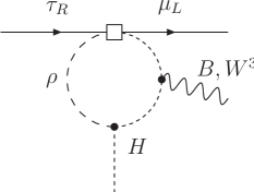
Figure 2: Example for 1-loop matching contribution to ${\cal O}_{\rm eff}$ in (3.2). Here $\rho$ is the heavy scalar degree of freedom appearing in the spurion $\xi_{E_{R}}$, which interacts with the SM Higgs and charged leptons through the scalar potential and the dimension-5 Yukawa terms (2.36).

After changing to the mass eigenbasis for the charged leptons, using (2.35, 2.44), the effective operator (3.2) exhibits the flavour structure

$$\left(V_{L}\,\Xi_{L}\,\xi_{E_{R}}^{\dagger}\right)_{ij}=U_{i3}U_{j3}^{*}\,(y_{\ell})_{j}\,\Lambda_{E}\,,$$ (3.3)

which reproduces the leading term for the result discussed in [2], in the limit $\Delta m^{2}_{\rm sol.}\ll\Delta m^{2}_{\rm atm.}$. The expression can be traced back to the effective quantity

$$\hat{\Delta}=V_{L}\,\hat{g}_{\nu}^{\dagger}\hat{g}_{\nu}V_{L}^{\dagger}-1/3\,{\rm tr}(\hat{g}_{\nu}^{\dagger}\hat{g})=\frac{\Lambda_{\rm LN}^{2}}{v^{4}}\left(U_{\rm PMNS}\,{\rm diag}[m_{\nu}^{2}]\,U_{\rm PMNS}^{\dagger}-\frac{1}{3}\,{\rm tr}[m_{\nu}^{2}]\right)\,,$$ (3.4)

which in the limit $m_{\nu_{3}}\gg m_{\nu_{1,2}}$ is given by, cf. (2.12),

$$\hat{\Delta}_{ij}\ \stackrel{{\scriptstyle m_{\nu_{3}}\gg m_{\nu_{1,2}}}}{{\longrightarrow}}\ g^{2}\left(U_{i3}U_{j3}^{*}-\frac{\delta_{ij}}{3}\right)\ \simeq\ \frac{g^{2}}{6}\left(\begin{array}[]{ccc}-2&0&0\\ 0&1&-3\\ 0&-3&1\end{array}\right)_{ij}\,,$$ (3.8)

where in the last line we inserted the approximation of the PMNS matrix for tri-bimaximal mixing (2.48). Sub-leading effects are induced by $g_{\nu}^{(2)}$, which can be seen by either including the corresponding $1/\Lambda$ corrections in (3.4), or by directly inserting additional powers of $g_{\nu}^{(2)}$ in effective operators like (3.2) as allowed by flavour symmetry. The discussion for the inverted hierarchy is completely analogous with, cf. (2.56),

$$\hat{\Delta}_{ij}\ \stackrel{{\scriptstyle m_{\nu_{3}}\ll m_{\nu_{1,2}}}}{{\longrightarrow}}\ g^{2}\left(\frac{\delta_{ij}}{3}-U_{i3}U_{j3}^{*}\right)\ \simeq\ \frac{g^{2}}{6}\left(\begin{array}[]{ccc}2&0&0\\ 0&-1&3\\ 0&3&-1\end{array}\right)_{ij}\,.$$ (3.12)

Finally, for degenerate neutrino masses we obtain $\hat{\Delta}\to 0$.

3.2 Example: 4-lepton processes

Flavour-violating 4-lepton processes are interesting, because different chirality structures can be experimentally constrained by a Dalitz-plot analysis and/or angular distributions [15, 16, 17], and this information may be used to distinguish between different NP models.

In the linear version of MLFV, see [2, 15], besides the effective quantity $\hat{\Delta}_{ij}$ discussed in the previous subsection, additional flavour structures arise, which can be expressed in terms of the tensor $G_{ij}^{kl}$, describing the 27-plet in the reduction of $(\bar{6},1)\times(6,1)=1+8+27$,

$$\hat{G}_{ij}^{kl} = (V_{L}^{*}\hat{g}_{\nu}V_{L}^{\dagger})_{ij}\,(V_{L}\hat{g}_{\nu}^{*}V_{L}^{T})^{kl}-\frac{1}{12}\left(\delta_{i}^{k}\delta_{j}^{l}+\delta_{i}^{l}\delta_{j}^{k}\right){\rm tr}(\hat{g}_{\nu}^{\dagger}\hat{g}_{\nu})$$ (3.13)

$${}-\frac{1}{5}\left(\delta_{i}^{a}\delta_{b}^{l}\delta_{j}^{k}+\delta_{j}^{a}\delta_{b}^{l}\delta_{i}^{k}+\delta_{i}^{a}\delta_{b}^{k}\delta_{j}^{l}+\delta_{j}^{a}\delta_{b}^{k}\delta_{i}^{l}\right)\,\hat{\Delta}^{b}{}_{a}\,.$$

Here $\hat{G}_{ij}^{kl}=\hat{G}_{ji}^{kl}=\hat{G}_{ij}^{lk}$, and $\sum_{i}\,\hat{G}_{ij}^{il}=0$. The 27-plet appears in purely left-handed operators as

$$G_{ij}^{kl}\,(\bar{L}_{k}\,L^{i})(\bar{L}_{l}\,L^{j})\,.$$

In the non-linear version of MLFV, the discussion is somewhat different. The elementary flavour-symmetry invariant building blocks for the leading left-handed operators are

$$(\bar{L}\,L)\,,\qquad(\bar{L}\,\Xi_{L})\,,\qquad(\Xi_{L}^{\dagger}L)\,.$$ (3.14)

After changing to the mass eigenbasis, the first term remains flavour diagonal, whereas

$$(\bar{L}\,\Xi_{L})\to(\bar{L}\,V_{L}\,\Xi_{L})=\bar{L}_{i}\,U_{i3}\,,$$ (3.15)

$$(\Xi_{L}^{\dagger}\bar{L})\to(\Xi_{L}^{\dagger}\,V_{L}^{\dagger}\,\Xi_{L})=U^{*}_{j3}\,L_{j}\,,$$ (3.16)

generate the same flavour factors as in $\hat{\Delta}_{ij}$ in (3.3). At tree level, the leading flavour coefficients in purely left-handed 4-lepton operators are thus determined by structures like

$$\frac{1}{\Lambda_{\rm LN}^{2}}\,(\bar{L}\,\gamma_{\mu}\,L)\,(\bar{L}\,\Xi_{L})\,\gamma^{\mu}\,(\Xi_{L}^{\dagger}L)\,,$$ (3.17)

$$\frac{1}{\Lambda_{\rm LN}^{2}}\,(\bar{L}\,\Xi_{L})\,\gamma_{\mu}\,(\Xi_{L}^{\dagger}L)\,\gamma^{\mu}\,(\bar{L}\,\Xi_{L})\,(\Xi_{L}^{\dagger}L)\,.$$ (3.18)

Loop diagrams, contributing to flavour-violating 4-lepton processes and involving the heavy degrees of freedom associated with the breaking of $G_{F}^{\prime}$ at the scale $\Lambda^{\prime}$, require at least two insertions of $1/\Lambda_{\rm LN}$ suppressed operators. For instance, in the case of normal hierarchy, we obtain terms like

$$\frac{1}{(4\pi\Lambda^{\prime})^{2}}\,(\bar{L}\,L)\,(\bar{L}\,{\cal U}_{L}^{(2)}\frac{\langle g_{\nu}^{(2)\dagger}g_{\nu}^{(2)}\rangle}{\Lambda_{\rm LN}^{2}}\,{\cal U}_{L}^{(2)\dagger}L)\,,$$ (3.19)

$$\frac{1}{(4\pi\Lambda^{\prime})^{2}}\,(\bar{L}\,L)\,(\bar{L}\,{\cal U}_{L}^{(2)}\frac{\langle Y_{E}^{(2)}Y_{E}^{(2)\dagger}\rangle}{\Lambda_{\rm LN}^{2}}\,{\cal U}_{L}^{(2)\dagger}L)\,,\quad\mbox{etc.}$$ (3.20)

Including right-handed fields, the leading tree-level flavour structures are obtained from 4-lepton operators of the form

$$\frac{1}{\Lambda_{\rm LN}^{2}}\,(\bar{E}_{R}\,E_{R})\,(\bar{L}\,\Xi_{L})\,(\Xi_{L}^{\dagger}L)\,.$$ (3.21)

Again, insertions of sub-leading operators in loop diagrams with heavy spurion degrees of freedom lead to additional structures, like

$$\frac{1}{(4\pi\Lambda^{\prime})^{2}}\,(\bar{E}_{R}\,\frac{\langle\xi_{E_{R}}\xi_{E_{R}}^{\dagger}\rangle}{\Lambda_{\rm LN}^{2}}\,E_{R})\,(\bar{L}\,L)\quad\mbox{etc.,}$$ (3.22)

and similarly for the inverted and degenerate case.

4 Beyond MLFV

A systematic procedure to include deviations from the MFV assumption within the ET framework (next-to-minimal flavour violation, nMFV) has been proposed in [6] (for alternative approaches, see [18, 19, 20]). However, the formalism has been worked out for quark decays in the linear formulation of MFV, only. In the following, we are going to apply the nMFV ansatz to the lepton sector within the non-linear formulation of lepton-flavour violation (nMLFV).

4.1 Normal hierarchy

	$E_{R}$	$({\cal U}_{L}^{(2)\dagger}L)$	$(\Xi_{L}^{\dagger}L)$	$({\cal U}_{L}^{(2)\dagger}L)^{*}$
$\bar{E}_{R}$	$Z_{E}\sim(1,8)_{0,0}$	$Y_{E}^{(2)\dagger}\sim(2,3)_{-1,0}$	$\xi_{E_{R}}\sim(1,3)_{0,1}$	$X_{E}^{(2)\dagger}\sim(2,3)_{1,0}$
$(\bar{L}\,{\cal U}_{L}^{(2)})$	$\bullet$	$Z_{L}^{(2)}\sim(3,1)_{0,0}$	$\chi_{L}\sim(2,1)_{1,1}$	$g_{\nu}^{(2)^{*}}\sim(3,1)_{2,0}$
$(\bar{L}\,\Xi_{L})$	$\bullet$	$\bullet$	$\sim(1,1)_{0,0}$	$\chi_{L}\sim(2,1)_{1,1}$
$(\bar{L}\,{\cal U}_{L}^{(2)})^{*}$	$\bullet$	$\bullet$	$\bullet$	$Z_{L}^{(2)}\sim(3,1)_{0,0}$

Table 1: Possible bi-linear combinations of fundamental fermion fields and the associated spurion fields (normal hierarchy, $G_{F}^{\prime}=SU(2)_{L}\times SU(3)_{E_{R}}\times U(1)_{L^{(2)}}\times Z_{2}$).

The basic idea of nMLFV is to introduce additional spurion fields that can couple to fundamental fermion bi-linears appearing in higher-dimensional gauge-invariant operators. Let us discuss the case of normal neutrino mass hierarchy, first. The basic fermion fields with definite transformations under $G_{F}^{\prime}$ are

$$E_{R}\sim(1,3)_{0,0}\,, ({\cal U}_{L}^{(2)\dagger}L)\sim(2,1)_{+1,0}\,,$$ (4.1)

$$(\Xi_{L}^{\dagger}L)\sim(1,1)_{0,1}\,, ({\cal U}_{L}^{(2)\dagger}L)^{*}\sim(2,1)_{-1,0}\,.$$ (4.2)

Out of these four fields, we can construct all possible bi-linear flavour structures, as shown in Table 1. In nMLFV each of these combinations corresponds to an independent spurion field. Besides the spurions $g_{\nu}^{(2)}$, $\xi_{E_{R}}^{\dagger}$ and $Y_{E}^{(2)}$, appearing in the non-linear formulation of MLFV, we also obtain new spurion fields $\chi_{L}$, $X_{E}^{(2)}$, $Z_{L}^{(2)}$ and $Z_{E}$. In nMLFV, we may thus consider new operators like, for instance,

$$\frac{1}{\Lambda^{2}}\,(\bar{L}\,{\cal U}_{L}^{(2)}\,\chi_{L}\,\gamma^{\mu}\,\Xi_{L}^{\dagger}L)\,(H^{\dagger}D_{\mu}H)\,,\quad\frac{1}{\Lambda^{2}}\,(\bar{L}\,{\cal U}_{L}^{(2)}\,\sigma^{\mu\nu}\,H\,X_{E}^{(2)}E_{R})\,B_{\mu\nu}\,,\quad\mbox{etc.}$$ (4.3)

Insertions of the spurion $\chi_{L}$ induce significant contributions to $\tau\to e\gamma$, where the leading MLFV contributions vanishes, because $U_{13}\simeq 0$, see (3.3,3.8). The spurions $Z_{E}$ and $X_{E}$ induce new lepton flavour-violating structures involving right-handed leptons. The set of new spurions can thus be used to parameterize deviations from the correlations between different LFV observables as one would predict in MLFV [21, 22].

As explained in [6], the new spurion fields can also appear in operators whose gauge structure is already present in MLFV, for instance

$$\frac{1}{\Lambda^{3}}\,\bar{N}^{T}{\cal U}_{L}^{(2)*}(\chi_{L}^{*}\,\chi_{L}^{\dagger})\ {\cal U}_{L}^{(2)\dagger}N\,.$$ (4.4)

A minimal constraint on the new spurion fields then follows from self-consistency relations for those combinations of old and new spurion fields that transform as the original MLFV spurions. As a consequence, the power-counting for the new spurion fields is limited from above by the phenomenology of lepton masses and mixing. In this context, an advantage of the non-linear formulation of MFV is that products of spurion fields in the effective Lagrangian are always suppressed by higher powers of $1/\Lambda$ compared to single spurion insertions. Therefore, we can safely restrict the discussion to products of two spurion fields. In the case of normal hierarchy this yields the following set of inequalities:

$$\left(\frac{g_{\nu}^{2}}{\Lambda}\right)_{ij} \gtrsim\ \left\{\left(\frac{\chi_{L}^{*}\,\chi_{L}^{\dagger}}{\Lambda^{2}}\right)_{ij}\,,\left(\frac{X_{E}^{(2)}\,Y_{E}^{(2)\dagger}}{\Lambda^{2}}\right)_{ij}\right\}\,,$$

$$\left(\frac{\xi_{E_{R}}^{\dagger}}{\Lambda}\right)_{ij} \gtrsim\ \left\{\left(\frac{\chi_{L}^{\dagger}Y_{E}^{(2)}}{\Lambda^{2}}\right)_{ij}\,,\left(\frac{\chi_{L}^{T}X_{E}^{(2)}}{\Lambda^{2}}\right)_{ij}\right\}\,,$$

$$\left(\frac{Y_{E}^{(2)}}{\Lambda}\right)_{ij} \gtrsim\ \left\{\left(\frac{\chi_{L}\,\xi_{E_{R}}^{\dagger}}{\Lambda^{2}}\right)_{ij}\,,\left(\frac{\phi_{1,2}\,X_{E}^{(2)}}{\Lambda^{2}}\right)_{ij}\right\}\,,$$ (4.5)

where we have not quoted “trivial” inequalities involving $Z_{L}^{(2)}$ and $Z_{E}$. The relations (4.5) are understood to hold order-of-magnitude-wise for a generic basis (i.e. where the off-diagonal entries of rotation matrices to the mass eigenbasis are of natural size).

4.2 Inverted hierarchy

	$E_{R}$	$({\cal U}_{L}^{(2)\dagger}L)$	$(\Xi_{L}^{\dagger}L)$
$\bar{E}_{R}$	$Z_{E}\sim(1,8)_{0}$	$Y_{E}^{(2)\dagger}\sim(2,3)_{0}$	$\xi_{E_{R}}\sim(1,3)_{-1}$
$(\bar{L}\,{\cal U}_{L}^{(2)})$	$\bullet$	$\tilde{g}_{\nu}^{(2)}\sim(2,1)_{0}$	$\chi_{L}\sim(2,1)_{-1}$
$(\bar{L}\,\Xi_{L})$	$\bullet$	$\bullet$	$\sim(1,1)_{0}$

Table 2: Possible bi-linear combinations of fundamental fermion fields and the associated spurion fields (inverted hierarchy, $G_{F}^{\prime}=SO(2)_{L}\times SU(3)_{E_{R}}\times U(1)_{L_{3}}$).

The situation is slightly simpler in the case of inverted hierarchy, where the basic fermion fields with definite transformations under $G_{F}^{\prime}$ are

$$E_{R}\sim(1,3)_{0}\,,\qquad({\cal U}_{L}^{(2)\dagger}L)\sim(2,1)_{0}\,,\qquad(\Xi_{L}^{\dagger}L)\sim(1,1)_{1}\,.$$ (4.6)

This implies the nMLFV spurion representations in Table 2, which only introduces two new spurion fields, $\chi_{L}$ and $Z_{E}$. In this case, the non-trivial inequality constraints for $\chi_{L}$ are obtained as

$$\left(\frac{\tilde{g}_{\nu}^{(2)}}{\Lambda}\right)_{ij} \gtrsim\ \left\{\left(\frac{\chi_{L}\,\chi_{L}^{\dagger}+\chi_{L}^{*}\chi_{L}^{T}}{\Lambda^{2}}\right)_{ij}\,,\left(\frac{(Y_{E}^{(2)}\,Y_{E}^{(2)\dagger})+(\cdots)^{T}-{\rm tr}(\cdots)}{\Lambda^{2}}\right)_{ij}\right\}\,,$$

$$\left(\frac{\xi_{E_{R}}^{\dagger}}{\Lambda}\right)_{ij} \gtrsim\ \left(\frac{\chi_{L}^{T}Y_{E}^{(2)}}{\Lambda^{2}}\right)_{ij}\,,\qquad\left(\frac{Y_{E}^{(2)}}{\Lambda}\right)_{ij}\gtrsim\ \left(\frac{\chi_{L}\,\xi_{E_{R}}^{\dagger}}{\Lambda^{2}}\right)_{ij}\,.$$ (4.7)

4.3 Degeneracy

Finally, for the case of degenerate neutrino masses, before the breaking of $G_{F}^{\prime}\to G_{F}^{\prime\prime}$, the nMLFV scheme reads

	$E_{R}\sim(1,3)$	$({\cal U}_{L}^{\dagger}L)\sim(3,1)$
$\bar{E}_{R}$	$Z_{E}\sim(1,8)$	$Y_{E}^{\dagger}\sim(3,3)$
$(\bar{L}\,{\cal U}_{L})$	$\bullet$	$\check{g}_{\nu}\sim(5,1)+Z_{L}\sim(3,1)$

which introduces the new spurions $Z_{E}$ and $Z_{L}$ with “trivial” inequality constraints. Applying the nMLFV construction to the ET after the breaking of $G_{F}^{\prime\prime}$, we obtain

	$E_{R}\sim(1,3)_{0}$	$(\check{\cal U}_{L}^{(2)\dagger}L)\sim(2,1)_{0}$	$(\check{\Xi}_{L}^{\dagger}L)\sim(1,1)_{1}$
$\bar{E}_{R}$	$Z_{E}\sim(1,8)_{0}$	$\check{Y}_{E}^{(2)\dagger}\sim(2,3)_{0}$	$\check{\xi}_{E_{R}}\sim(1,3)_{1}$
$(\bar{L}\,\check{\cal U}_{L}^{(2)})$	$\bullet$	$\check{g}_{\nu}^{(2)}\sim(2,1)_{0}$	$\check{\chi}_{L}\sim(2,1)_{1}$
$(\bar{L}\,\check{\Xi}_{L})$	$\bullet$	$\bullet$	$\sim(1,1)_{0}$

which has a similar form as for the inverted hierarchy case, only the $U(1)_{L_{3}}$ quantum numbers are replaced by $Z_{2}$ ones.

As a final remark, we should also point out that the nMFV framework would allow for spurion fields that transform under both, the quark and the lepton-flavour symmetry group, and could be a remnant of lepto-quark interactions which typically appear in grand-unified theories. A detailed discussion of the potential consequences and phenomenological constraints is beyond the scope of this work.

5 Summary

Non-linear realizations of flavour symmetry are advantageous in cases where very distinct eigenvalues of Yukawa or Majorana mass matrices appear. For the quarks, it is the large Yukawa coupling of the top which breaks the $SU(3)^{3}$ flavour symmetry down to $SU(3)\times SU(2)^{2}\times U(1)$, where the latter symmetry is only weakly broken by the remaining small Yukawa couplings. In this paper we have used the same reasoning to discuss the flavour symmetries of leptons. Here the hierarchy in the neutrino mass differences, $\Delta m^{2}_{\rm sol}\ll\Delta m^{2}_{\rm atm}$, can be used to construct a parameterization of the effective Majorana mass matrix (entering the dim-5 operator in a scenario with only left-handed neutrinos) which reflects the non-linear realization of lepton flavour symmetry.

We have considered the various possible scenarios for neutrino-mass hierarchies, and for each case we have determined the residual symmetries, after the largest entries in the Majorana mass matrix have been identified. The remaining entries are parameterized in terms of Goldstone modes for the broken generators, and spurion fields which eventually break the residual flavour symmetry. Based on the minimal flavour violation hypothesis, we may then construct the flavour structure of possible New Physics operators which mediate e.g. lepton-flavour violating decays of charged leptons. Within the same framework, we have also considered possible parameterizations of “next-to-minimal lepton flavour violation” along the lines proposed in [6].

Besides offering a systematic model-independent framework to discuss deviations from the Standard Model in lepton-flavour violating processes, our approach also provides some new perspectives on the flavour puzzle within the Standard Model and beyond. In particular, it is interesting to note that the different possible realizations of mass hierarchies for neutrinos and charged leptons is unambiguously linked to different sequences of flavour symmetry breaking, $G_{F}\to G_{F}^{\prime}\to G_{F}^{\prime\prime}\to\ldots$ (A similar statement holds for the quark sector, which is going to be explored in a future publication).

Acknowledgements

We thank Wolfgang Kilian and Werner Rodejohann for helpful discussions. This work is partially supported by the German Research Foundation (DFG, Contract No. MA1187/10-1) and by the German Ministry of Research (BMBF, Contract No. 05HT6PSA).

References

- [1] G. D’Ambrosio, G. F. Giudice, G. Isidori and A. Strumia, Nucl. Phys. B 645, 155 (2002) [hep-ph/0207036].
- [2] V. Cirigliano, B. Grinstein, G. Isidori and M. B. Wise, Nucl. Phys. B 728 (2005) 121 [hep-ph/0507001]; V. Cirigliano and B. Grinstein, Nucl. Phys. B 752 (2006) 18 [hep-ph/0601111].
- [3] M. Ciuchini, G. Degrassi, P. Gambino and G. F. Giudice, Nucl. Phys. B 534, 3 (1998) [hep-ph/9806308].
- [4] A. J. Buras, P. Gambino, M. Gorbahn, S. Jäger and L. Silvestrini, Phys. Lett. B 500, 161 (2001) [hep-ph/0007085].
- [5] Th. Feldmann and Th. Mannel, Phys. Rev. Lett. 100, 171601 (2008) [arXiv:0801.1802 [hep-ph]].
- [6] Th. Feldmann and Th. Mannel, JHEP 0702, 067 (2007). [hep-ph/0611095].
- [7] R. D. Peccei and H. R. Quinn, Phys. Rev. D 16, 1791 (1977).
- [8] B. Pontecorvo, Sov. Phys. JETP 26 (1968) 984 [Zh. Eksp. Teor. Fiz. 53 (1967) 1717].
- [9] Z. Maki, M. Nakagawa and S. Sakata, Prog. Theor. Phys. 28 (1962) 870.
- [10] P. F. Harrison, D. H. Perkins and W. G. Scott, Phys. Lett. B 530 (2002) 167 [hep-ph/0202074].
- [11] S. Choubey and W. Rodejohann, Eur. Phys. J. C 40 (2005) 259 [hep-ph/0411190].
- [12] M. Maltoni, T. Schwetz, M. A. Tortola and J. W. F. Valle, New J. Phys. 6 (2004) 122 [hep-ph/0405172]; M. C. Gonzalez-Garcia and M. Maltoni, arXiv:0704.1800 [hep-ph].
- [13] S. R. Coleman, J. Wess and B. Zumino, Phys. Rev. 177, 2239 (1969); C. G. Callan, S. R. Coleman, J. Wess and B. Zumino, Phys. Rev. 177, 2247 (1969).
- [14] S. Davidson and F. Palorini, Phys. Lett. B 642 (2006) 72 [hep-ph/0607329].
- [15] B. M. Dassinger, Th. Feldmann, Th. Mannel and S. Turczyk, JHEP 0710 (2007) 039 [arXiv:0707.0988 [hep-ph]].
- [16] A. Matsuzaki and A. I. Sanda, Phys. Rev. D 77 (2008) 073003 [arXiv:0711.0792 [hep-ph]].
- [17] M. Giffels, J. Kallarackal, M. Kramer, B. O’Leary and A. Stahl, Phys. Rev. D 77 (2008) 073010 [arXiv:0802.0049 [hep-ph]].
- [18] K. Agashe, M. Papucci, G. Perez and D. Pirjol, hep-ph/0509117.
- [19] A. L. Fitzpatrick, G. Perez and L. Randall, arXiv:0710.1869 [hep-ph].
- [20] S. Davidson, G. Isidori and S. Uhlig, arXiv:0711.3376 [hep-ph].
- [21] V. Cirigliano and B. Grinstein, Nucl. Phys. B 752 (2006) 18 [hep-ph/0601111].
- [22] G. C. Branco, A. J. Buras, S. Jäger, S. Uhlig and A. Weiler, JHEP 0709 (2007) 004 [hep-ph/0609067].