Detection of quiescent galaxies in a bicolor sequence from $z=0-2$

Abstract

We investigate the properties of quiescent and star–forming galaxy populations to $z\sim 2$ with purely photometric data, employing a novel rest–frame color selection technique. From the UKIDSS Ultra–Deep Survey Data Release 1, with matched optical and mid–IR photometry taken from the Subaru XMM Deep Survey and Spitzer Wide–Area Infrared Extragalactic Survey respectively, we construct a $K$–selected galaxy catalog and calculate photometric redshifts. Excluding stars, objects with uncertain $z_{\rm phot}$ solutions, those that fall in bad or incomplete survey regions, and those for which reliable rest–frame colors could not be derived, 30108 galaxies with $K<22.4$ (AB) and $z_{\rm phot}\leq 2.5$ remain. The galaxies in this sample are found to occupy two distinct populations in the rest–frame $U-V$ vs. $V-J$ color space: a clump of red, quiescent galaxies (analogous to the red sequence) and a track of star–forming galaxies extending from blue to red $U-V$ colors. This bimodal behavior is seen up to $z\sim 2$. Due to a combination of measurement errors and passive evolution, the color–color diagram is not suitable to distinguish the galaxy bimodality at $z>2$ for this sample, but we show that MIPS 24$\mu$m data suggest that a significant population of quiescent galaxies exists even at these higher redshifts. At $z=1-2$, the most luminous objects in the sample are divided roughly equally between star–forming and quiescent galaxies, while at lower redshifts most of the brightest galaxies are quiescent. Moreover, quiescent galaxies at these redshifts are clustered more strongly than those actively forming stars, indicating that galaxies with early–quenched star formation may occupy more massive host dark matter halos. This suggests that the end of star formation is associated with, and perhaps brought about by, a mechanism related to halo mass.

1. Introduction

The stellar mass in the local universe lies largely within two distinct classes of galaxies: actively star–forming spirals, and massive ellipticals with evolved stellar populations and little current star formation. These populations show strongly bimodal behavior in a number of measured and derived quantities, including color (Baldry et al., 2004), the 4000Å–break strength $D_{n}(4000)$ (an indicator of stellar population age; Kauffmann et al., 2003), and clustering strength (Budavari et al., 2003). Relatively low–mass galaxies with high star–formation rates have also been found at high redshifts (e.g., $z>3$ Lyman–break galaxies or LBGs; Steidel et al., 1996). Surprisingly, the population of massive, “dead” galaxies appears to persist to high redshift as well (e.g. Labbé et al., 2005; Daddi et al., 2005; Kriek et al., 2006, 2008b), even though the universe was only a few Gyr old at that point. Since the stellar populations of evolved galaxies often have ages that are a significant fraction of the age of the universe at these redshifts, the implication is that they must have formed (and their star formation ceased) far earlier than anticipated by standard hierarchical structure formation models.

Investigating the evolution of star formation activity and the assembly of stellar mass over the past $\sim 12$ Gyr are therefore two key avenues to understanding how the present galaxy population came to be, and large samples of galaxies during this peak formation epoch ($z\sim 2$) are needed for this. As spectroscopy of faint objects is extremely expensive with regard to telescope time, several highly efficient broadband selection techniques have been designed to weed out low–redshift interlopers. In addition to the aforementioned LBG selection, which primarily finds unobscured star–forming galaxies at $z>3$, the distant red galaxy (DRG) criterion ($J-K>2.3$ (Vega) or $>1.34$ (AB); Franx et al., 2003) instead tends to find the most massive galaxies at $2<z<3$ (van Dokkum et al., 2006), about half of which show signs of heavily–obscured star formation (Papovich et al., 2006). Other methods, such as the $BzK$ selection of Daddi et al. (2004), are adept at selecting $z\sim 2$ galaxies over a wide range of masses and star–formation rates.

Each of these techniques has its advantages and disadvantages, but one point has become clear: to effectively study the mass evolution of high–redshift galaxies, deep near–infrared data are crucial. The observed $JHK$ bands trace rest–frame optical light at $z\sim 2-3$ and provide a more reliable indicator of stellar mass than the rest–frame UV (observed optical); indeed, DRGs themselves appear to represent an important fraction, if not the majority, of stellar mass at high redshifts (Rudnick et al., 2006; Grazian et al., 2007). Such galaxies are typically faint in the observed optical bands, either from old stellar populations or dust obscuration, and are often missed by purely optical selection techniques (Quadri et al., 2007b). Selecting galaxies from deep near–infrared fields is therefore likely to yield a more complete picture of the stellar mass at high redshift than similar studies at optical wavelengths.

Until recently, the small sizes (at most a few square arcminutes) and relatively low efficiencies of the available infrared detectors made large, deep near–IR surveys impractical. Such projects therefore typically followed the “pencil–beam” approach, surveying a single frame to high sensitivity (e.g., the Faint Infrared Extragalactic Survey, FIRES; Franx et al., 2003), or alternatively observing somewhat larger areas at the expense of depth (e.g., GOODS–S; Giavalisco et al., 2004). While such surveys have revealed a great deal about the high–redshift universe, the necessarily small survey volumes proved problematic for statistical studies of galaxy populations (as a result of both cosmic variance and small–number statistics).

Large–format near–IR detectors on 4m–class telescopes (such as ISPI, WFCAM, and the upcoming VISTA camera) now provide the ability to conduct deep surveys over wide areas, and a number of past, present, and planned projects take advantage of this capability – examples include the Multiwavelength Survey by Yale–Chile (MUSYC; Gawiser et al., 2006; Quadri et al., 2007b), the UKIRT Infrared Deep Sky Survey (UKIDSS; Lawrence et al., 2007), and ULTRA–VISTA. Until this latter survey is complete, the UKIDSS Ultra–Deep Survey (UDS) is the premier near–IR dataset in terms of depth and area. Overlapping deep optical imaging from the Subaru–XMM Deep Survey (SXDS; Sekiguchi et al., 2004) and shallow mid–IR data from the Spitzer Wide–Area Infrared Extragalactic (SWIRE; Lonsdale et al., 2003) survey provide complementary data over a broad range of wavelengths.

Here we derive a multiband $K$–selected galaxy catalog from the UDS, SXDS, and SWIRE data, calculating photometric redshifts and rest–frame colors for all objects in the overlapping survey area. Rather than rely on a specific color selection technique, we instead define samples of galaxies at various redshifts directly from the computed $z_{\rm phot}$ values, and further subdivide the samples into star–forming and quiescent galaxies based on their rest–frame colors. The color evolution with redshift, and the clustering of $1<z_{\rm phot}<2$ galaxies, are then determined. Readers who are primarily interested in these science results can find this discussion beginning in §6.

We present an overview of the survey data in §2, and the process of preparing and matching the datasets to each other in §3. The extraction of the catalog is then discussed in §4, and the derivation of photometric redshifts and rest–frame colors in §5. §6 describes the bimodality of galaxies in rest–frame color space and the separation into quiescent and star–forming samples, and the clustering properties of these two populations are discussed in §7. Further discussion, caveats, and a summary of the results can then be found in §8, §9, and §10 respectively.

A cosmology with $H_{0}=70$ km s^-1 Mpc^-1, $\Omega_{m}=0.3$, and $\Omega_{\Lambda}=0.7$ is assumed throughout, and magnitudes are quoted in the AB system unless otherwise noted.

2. Data characteristics

In this analysis we employ the reduced $J$– and $K$–band UDS mosaics provided as a subset of the UKIDSS Data Release 1 (DR1; Warren et al., 2007a); $H$–band data were not available in this release. The UKIDSS project, defined in Lawrence et al. (2007), uses the UKIRT Wide Field Camera (WFCAM Casali et al., 2007) and a photometric system described in Hewett et al. (2006); the pipeline processing and science archive are described in Irwin et al. (in preparation) and Hambly et al. (2008) respectively. The UDS field consists of a single repeatedly–observed UKIDSS survey tile (in turn comprising four subsequent WFCAM observations arranged in a square to produce uniform coverage), with a total area of $0.77$ deg² and reaching nominal depths of $K<23.45$ and $J<23.55$ (AB; $5\sigma$ point–source threshold in a 2″ aperture). The 0$\farcs$4 pixel scale of WFCAM does not sufficiently sample the $K-$band PSF of $\sim 0\farcs 7$, so the individual observations are offset by fractions of a pixel and the combined mosaics regridded by a factor of 3 to a pixel scale of 0$\farcs$134. Note that while Data Release 2 has since been made available (Warren et al., 2007b), this release contains identical UDS mosaics to DR1; only data in the shallower UKIDSS surveys were updated.

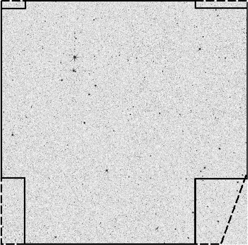
Figure 1.— UKIDSS $K$-band image of the UDS field, with SXDS (solid line) and SWIRE (dashed line) coverage overplotted. The image is about 52′ on a side; north is up and east is to the left.

Optical imaging of most of the UDS field is provided by the Subaru–XMM Deep Survey (SXDS) beta release, a deep wide–field survey employing the Subaru telescope and Subaru Prime Focus Camera (Suprime–Cam or SUP; Miyazaki et al., 2002). This imager contains ten $2048\times 4096$ pixel CCDs arranged in a $5\times 2$ mosaic, providing a rectangular field–of–view of roughly $34\arcmin\times 27\arcmin$. The SXDS then consists of five overlapping SUP fields arranged in a cross–shaped pattern (three adjacent fields in the north–south direction, and two on the eastern and western flanks with the camera rotated $90^{\circ}$; see Figure 1). Reported $5\sigma$ depths (in a 2″ aperture) are $B<27.5$, $R<26.8$, $i^{\prime}<26.5$, and $z^{\prime}<25.4$, though the sensitivity varies by $\sim 0.2$ between the five fields (with a $\sim 0.6$ mag variation in $z$); our independent sensitivity estimates are comparable to the reported values.

The SWIRE survey covers a total of $\sim 49$ deg² with IRAC and MIPS in six subfields, one of which (the XMM–LSS field) includes nearly the entire UDS/SXDS area. The orientations of the IRAC/MIPS fields are at an angle to the UDS; therefore, only a small triangular region in the southwest corner of the UDS has no SWIRE coverage (shown in Figure 1). SWIRE reaches nominal $5\sigma$ point–source depths of 3.7, 5.4, 48, and 37.8 $\mu$Jy in the 3.6, 4.5, 5.8, and 8.0 $\mu$m IRAC bands respectively, and 230 $\mu$Jy in MIPS 24 $\mu$m. The IRAC mosaics of this field are divided into 16 separate subimages, with four of these having some overlap with the UDS field; the MIPS 24 $\mu$m image of the field is available as a single file. The relevant subimages of all four IRAC bands, as well as the full 24 $\mu$m MIPS image, were obtained from the public SWIRE data website. Due to their far broader point–response functions and lower sensitivities, we do not analyze the MIPS 70 $\mu$m or 160 $\mu$m data here; similarly, the $5.8\mu$m and $8\mu$m data are excluded due to their order–of–magnitude lower sensitivity compared to the first two IRAC bands. Furthermore, since most objects seen in the UDS $K$–band are not individually detected in the SWIRE $24\mu$m image, the $24\mu$m data are therefore not included in our final $K$–selected catalog (but a stacking analysis of these data are discussed in §6.4). A summary of the data employed in the production of our $K$–selected catalog, including areas and measured limiting depths (as discussed in §4.5) is given in Table 1.

3. Data preparation

3.1. Image registration

The simplest way to achieve consistent flux measurements across multiple bands with arbitrary PSFs is to transform the images such that they are all on the same coordinate system and pixel scale. The pixel scale of the UDS images is 0$\farcs$134; however, all of these images have PSF FWHMs larger than 0$\farcs$7 (the UDS $K$–band seeing). To reduce file sizes and processing time, we thus adopt a standard pixel scale of 0$\farcs$202, the native scale of the SXDS images. This is somewhat coarser than the original regridded UDS pixel scale, but still sufficiently samples all PSFs.

The SWarp software package (Bertin et al., 2002) was used to crop, resample, and transform these sets of images to a common coordinate system before combining the subimages (in the cases of the IRAC and SXDS data) into single mosaics. Since the UDS $K$ image has the best seeing and is the band from which objects are detected, this was taken as the “standard” field to which all other images were registered. The $J$ and $K$ data were resampled to the SXDS pixel scale and cropped to remove noisy and missing data regions near the edges, resulting in 52$\farcm$4 by 53$\farcm$0 images. Likewise, the SWIRE MIPS 24 $\mu$m image and the IRAC subimages that cover the UDS field were transformed, resampled, and cropped to cover the same area. However, since the five SXDS pointings taken with each filter can exhibit different seeing and geometric distortions, those images were PSF–matched (see §3.2) and astrometrically corrected prior to combining with SWarp.

As SWarp transformed the images based solely on the astrometric information in the image FITS headers, some distortions are likely to remain (particularly between data from differing instruments). The measured positions of stars were thus used to correct these distortions. Source Extractor version 2.5.0 (SExtractor; Bertin & Arnouts, 1996) was first used to find the positions of bright objects in the $K$ image and measure their approximate $J$ and $K$ fluxes. $1179$ stars were selected on the basis of their blue IR colors ($J-K<0$) and bright but unsaturated $K$–band fluxes ($17.4<K<21.4$). The radial profiles of these objects were fitted with Gaussians to determine their centers and PSF widths in the $K$ band; all but a negligible fraction ($<1$%)had FWHMs comparable to the nominal image resolution, indicating that this simple color cut indeed primarily selects point sources. Next, a centroid algorithm was employed to determine the positions of these stars in each of the $BRi^{\prime}z^{\prime}JK/3.6/4.5$ images. Finally, the pixel positions of these stars along with the IRAF tasks geomap and geotran were used to transform the SXDS, UDS $J$, and IRAC images to the same coordinate system as the UDS $K$ mosaic. To check the agreement between the images, the pixel coordinates of these stars were again measured in the transformed images and found to agree well, e.g. in the $B$ mosaic the image coordinates agree with those in the $K$ image to within 0.5 pixel (0$\farcs$1) in 75% of cases, with a median absolute deviation of 0$\farcs$06. Similar offsets are seen in the transformed IRAC $3.6$ and $4.5\mu$m images (in addition, automatic astrometric corrections are performed in the IRAC deblending described in §4.2). Such astrometric deviations typically translate to systematic flux errors of at most $\sim 1$%.

3.2. IR/Optical PSF matching

The observed seeing width varies significantly between the different bands: point sources in the UDS have FWHMs of approximately 0$\farcs$7 in $K$ and 0$\farcs$8 in $J$, while in SXDS they range between $0\farcs 7-0\farcs 9$ depending on the field and band. Additional higher–order variations are likely to be present in the PSFs due to differences in the two instruments’ optics. Directly performing aperture photometry on these images would lead to flux offsets in the different bands (with less flux falling inside the aperture for the poorer–seeing images), and thus systematic color errors.

To mitigate this, all images were smoothed to the same PSF before fluxes were measured. Although this can be accomplished by convolving each with a simple Gaussian or higher–order kernel, the multitude of stars within these images can themselves be used to generate empirical kernels that contain all structural information about the PSFs. This is accomplished by deconvolving a low–resolution (“reference”) PSF with one constructed from a higher–resolution image:

$$K=P_{\rm ref}\otimes^{-1}P_{\rm hires}$$ (1)

where $P_{\rm ref}$ and $P_{\rm hires}$ are the low–resolution and high–resolution PSFs respectively. The resulting kernel can then be convolved with the high–resolution image in its entirety to bring it to the same PSF as the reference image.

$$I_{\rm match}(x,y)=I_{\rm hires}(x,y)\otimes K$$ (2)

Since the deconvolution step strongly magnifies any intrinsic noise in the PSFs, a large number of bright (but unsaturated) stars are necessary in each band to produce PSFs with sufficiently low noise levels.

For the $J$ and $K$ images, the PSFs were constructed from the same stars that were selected for astrometric matching, keeping the 200 brightest in each band. However, many of these stars are saturated in the SXDS images due to the much longer exposure times employed in this survey. As the effects of saturation are far more detrimental for the PSF shape than in the astrometric correction, a different method for selecting stars in the SXDS images is necessary. For these images, the IRAF psfmeasure task was used to estimate widths of unsaturated objects in the image based on a Gaussian fit. In a histogram of the widths of these objects, there is an obvious cutoff on the low–FWHM end accompanied by a sharp peak and an overlying broad distribution extending to larger FWHMs. Objects in the narrow peak were presumed to be point sources to within the image resolution, and the brightest of these were selected as stars in each optical image.

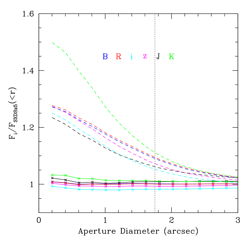
Figure 2.— Average growth curves of the six optical/IR bands divided by the growth curve of the worst image (SXDS–West $z$-band, with a PSF FWHM $\sim 0\farcs 9$). Relative growth curves before (dashed) and after (solid with points) convolution to the broadest PSF are shown. The vertical dotted line shows the “color” aperture size of 1$\farcs$75. Typical systematic flux errors due to PSF matching at this aperture size are $<2$%.

Square postage stamps (21 pixels or 4$\farcs$2 on a side) of the stars selected in each image were then created, and these in turn were median–combined to create 22 empirical PSFs (one for each of the 20 SXDS subimages, plus one for each UDS mosaic). Enclosed flux as a function of aperture size (growth curves) were then created for these PSFs. The “slowest–growing” growth curve, indicating the broadest PSF, is that of the western SXDS $z-$band image with a FWHM of $\sim 0\farcs 9$. Thus, we take this as the reference PSF and match the other 19 SXDS fields and two UDS images to it. The average growth curves for point sources in the smoothed $BRi^{\prime}z^{\prime}JK$ images, expressed as a fraction of the SXDS–West $z^{\prime}$ (reference) growth curve, before and after smoothing, are shown in Figure 2. At the aperture sizes used for flux measurements in the following section ($>1\farcs 75$ or $\sim 9$ pixels in diameter), the PSFs are matched to within 2%.

The point–response functions of the IRAC 3.6 $\mu$m and 4.5 $\mu$m images are roughly $1.7\times$ as broad as in the worst SXDS image ($\sim 1\farcs 6$ for both); they also contain significant non-Gaussian structure resulting from point source diffraction. While it would have been simpler in principle to smooth the $BRi^{\prime}z^{\prime}JK$ images to the IRAC PSF shape, this would substantially reduce the detection efficiency in $K$ while (for most high–redshift sources) providing only weak detections in IRAC to begin with. Additionally, blending from nearby sources is more likely to adversely affect simple aperture photometry in the IRAC images. PSF–matching and photometry are thus performed on these data using a different technique, described in §4.2.

4. Catalog extraction

4.1. Source detection and photometry

To measure fluxes of sources in the $BRi^{\prime}z^{\prime}JK$ images we used SExtractor in dual–image mode, whereby one image is used to detect sources and aperture photometry is performed on another image registered to the identical coordinate system. The unsmoothed (pre–PSF matching) $K$ mosaic was used as the detection image, and fluxes were measured in each of the six PSF–matched IR/optical mosaics. The sensitivity across the $K$ image is not perfectly uniform due to overlapping exposures and array efficiency variations; such nonuniformity can lead to corresponding variations in the number of detected galaxies, and thus to spurious clustering signals. We used the UKIDSS–supplied confidence map to construct an RMS map of the $K$ image, and this map was applied as the weight image within SExtractor in order to detect sources in an effectively noise–equalized and uniform manner. Several initial SExtractor runs were performed with varying detection parameters and the results checked by eye; the final choice of parameters appeared to find all faint objects with few spurious detections (see §4.5).

Figure 3.— Top panel: Median growth curves of point sources in the PSF–matched $BRi^{\prime}z^{\prime}JK$ images; Bottom panel: Signal–to–noise in the six bands, defined as the growth curve divided by the empty aperture noise function in each band, normalized to the peak SN in each band. The solid vertical line denotes the color aperture size of 1$\farcs$75.

Total fluxes were determined using a flexible elliptical aperture (SExtractor’s AUTO aperture; Kron, 1980). To ensure that color measurements are consistent, fluxes in a fixed circular aperture were also measured. The optimal size of this “color” aperture is subject to two primary considerations: while a larger aperture encloses a greater fraction of a given object’s flux, it also suffers from higher uncertainty due to background fluctuations. To determine the best aperture size, we divided the growth curve of each image by its noise function (i.e., photometric uncertainty versus aperture size, described in detail in §4.4). This is effectively equivalent to the signal–to–noise (SN) of each image as a function of aperture size, and is shown in the lower panel of Figure 3.

The $K$–band SN peaks at a diameter of $\sim 4$ pixels or 0$\farcs$8, which is lower than the ideal aperture size theoretically expected with uncorrelated noise ($\sim 1\farcs 0$), but consistent with the $1.1-1.4\times$FWHM optimal aperture found for the MUSYC data (Quadri et al., 2007b). The growth curves shown in the top panel of Figure 3 indicate that an aperture of this size misses about 70% of a point source’s flux. Such a small aperture is highly susceptible to systematic errors from imperfect PSF matching and astrometric offsets. Additionally, larger apertures appear to produce slightly bluer $J-K$ colors (on the order of 0.05 magnitudes between 1″ and 2″ apertures), perhaps due to intrinsic galaxy color gradients and/or imperfect image matching. To ensure more accurate colors of non–point sources, as a compromise we adopt a somewhat larger “color” aperture of 1$\farcs$75 diameter. This more than doubles the enclosed flux while only decreasing the SN by $\sim 30$% from the optimal value.

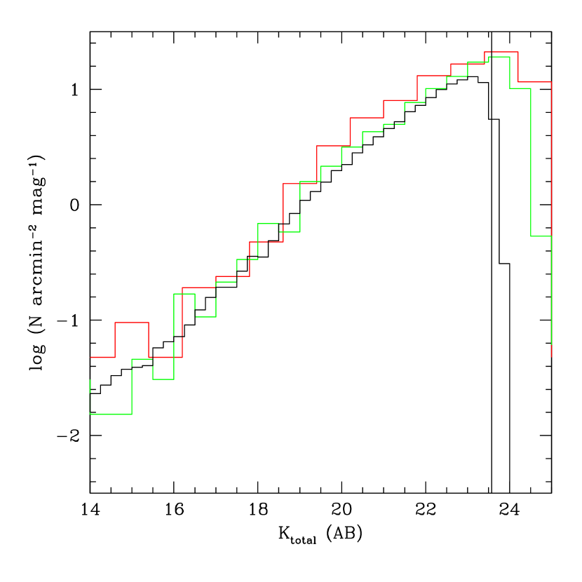
Figure 4.— Distribution of total $K$ magnitudes for objects in the UDS $K$-selected catalog detected at $>5\sigma$ significance in the “color” (1$\farcs$75 diameter) aperture black histogram. The vertical black line indicates the mean $5\sigma$ detection limit of $K=23.57$. Overplotted are raw number counts from the FIRES MS1054-03 cluster field (Förster Schreiber et al., 2006, red histogram) and the CDFS–GOODS $K$-selected catalog (Wuyts et al., 2008, green histogram).

In cases where the AUTO aperture is smaller than 1$\farcs$75 (primarily occurring for faint, point–like sources), the color aperture flux is substituted for the total flux. All total fluxes are corrected for flux falling outside the aperture assuming a minimal (point–like) source flux distribution. The SExtractor photometry was verified by comparing the $z^{\prime}$ total flux values with those of objects in spatially coincident HST/ACS images. The only useful ACS data in the archive were taken with the F850LP filter, which is approximately equivalent to SXDS $z^{\prime}$; fluxes of objects in these ACS data were consistent with those derived from SXDS. The photometric zeropoints of the SXDS $z^{\prime}$ data thus appear to be properly calibrated. Since the same calibration techniques and standard star fields were used by the SXDS team to determine the $BRi^{\prime}$ image zeropoints, we assume the calibrations in these bands are accurate as well (though the lack of available verification data should be kept in mind). Figure 4 shows the distribution of $K$ magnitudes for all objects detected by SExtractor, with number counts overplotted from two other $K$–selected samples: FIRES MS1054-03 (Förster Schreiber et al., 2006) and CDFS-GOODS (Wuyts et al., 2008). The number counts of the three surveys are similar to the UDS limiting magnitude, though the enhanced number of faint objects in the FIRES field (due to the presence of the $z=0.83$ cluster MS $1054-03$) is evident.

4.2. IRAC PSF–matching and photometry

As previously mentioned, the optical and NIR images were smoothed to the seeing of the SXDS–West $z^{\prime}$–band data rather than the much broader point–response function of the IRAC data. The direct aperture photometry from SExtractor would therefore not measure IRAC fluxes that are properly matched to the other bands. Moreover, the lower–resolution IRAC images are more prone to blending than the other bands, which can introduce significant systematic errors in the measured colors. We thus employed the method of Labbé et al. (2006) to correct this, summarized below.

Sources that are bright in $K$ are also typically bright in the 3.6/4.5 $\mu$m bands; thus, the $K$ image is used as a high–resolution template to deblend the IRAC images. Convolution kernels used to transform from the $K$ to the IRAC PSFs are constructed from bright and unsaturated sources (computed by fitting a series of Gaussian–weighted Hermite functions to the Fourier transforms of the objects in IRAC and $K$), and a smoothed map of the kernel coefficients as a function of image position is then produced. For a given object detected in $K$, neighboring sources are fitted and subtracted out using the local convolution kernel (derived from the aforementioned smoothed coefficient map) and the SExtractor–derived segmentation map. This results in a “cleaned” IRAC subimage containing only the source in question; standard photometry with a 3″ diameter aperture is then performed on the source, and this process is repeated for each object in the $K$–selected catalog. Through a visual inspection of the IRAC residual image with all sources subtracted, we conclude that this method effectively removes contaminating sources (for an illustration of this technique, see also Figure 1 in Wuyts et al., 2007).

Since the IRAC photometry from this procedure is performed using a larger aperture on images with significantly broader PSFs than the matched $BRi^{\prime}z^{\prime}JK$ images, these fluxes must be corrected in order to obtain accurate IRAC–IR/optical colors. This is accomplished by multiplying the IRAC flux measured in a 3″ aperture by a correction factor to obtain a “matched” IRAC flux:

$$f_{\rm IRAC,match}=f_{\rm IRAC}(3\arcsec)\times\frac{f_{\rm K}(1\farcs 75)}{f_{\rm K,conv}(3\arcsec)}$$ (3)

where $f_{\rm K,conv}$(3″) is the flux of the object measured in the $K$–band image after smoothing it to the IRAC resolution, and $f_{\rm K}$ is the K–band flux measured in the fixed “color” aperture (see §4.1). This correction implicitly assumes that the ratio of fluxes between the two aperture sizes is the same for $K$ and IRAC, i.e. color gradients between 1$\farcs$75 and 3″ are insignificant. While this technique could introduce systematic errors in measurements of extended sources with strong color gradients, at the redshifts primarily considered here ($z\gtrsim 1$) most galaxies have small angular sizes and are not likely to be adversely affected.

4.3. Bad pixels

All three sets of images (UDS, SXDS, SWIRE) contained regions where either no data were available or the derived photometry was unreliable. Thus, even though SExtractor finds objects in these regions, their fluxes should be considered unreliable. To account for this we created bad–pixel maps for each image set; if an object’s “color” aperture contains any such bad pixels, we set a flag indicating as such in the catalog. The bad pixel maps created for each survey are mostly a result of the following effects:

1. UDS $JK$:False sources and large negative residuals. In rows and columns containing bright stars, there are often significant positive and negative images (repeated at regular intervals) as a result of crosstalk between WFCAM detector nodes. These “false positive” images, while obviously not true astrophysical sources upon visual inspection, are nonetheless picked up as real objects by SExtractor. To make matters worse, many such “false positives” in $K$ have negative apparent flux in $J$, causing these to appear as very red objects. They can thus mimic high–redshift near–IR galaxy colors and may be an important contaminant in our catalog. Fortunately, adjacent to most of the false positive images in $K$, some strongly negative residuals are also typically seen. We thus searched for such strong $K$ residuals in the image, removing any object falling on or within 10 pixels of any such artifact as bad. As a secondary check, we searched for objects which were detected in $K$ but undetected in the sum of the $B+R+i^{\prime}+z^{\prime}$ mosaics. This cut finds an additional $\sim 1900$ possible bad spots. A visual inspection confirms that about $80$% of these are indeed artifacts (including diffraction spikes from bright stars and meteor streaks in $K$) that were undetected by the aforementioned “negative residual” technique, and most of the remaining $20$% are extremely faint and likely to be spurious detections. However, since some of these optically–nondetected objects are real, they have been included in the catalog with a flag indicating that they are likely to be bad.

2. SXDS $BRi^{\prime}z^{\prime}$: Non–covered regions and bright stars. As shown in Figure 1, the corners of the $UDS$ fields are not covered by the SXDS imaging. Additionally, bright stars in SXDS are surrounded by concentric halos and extended readout streaks. The Subaru team has provided files which define the regions affected by these bright stars; a visual inspection of the SXDS frames confirms that these regions accurately describe the affected areas. For each of the five pointings we created a map such that pixels falling within these regions had a value of 1, and zero otherwise. Using SWarp, these bad pixel masks were then transformed and combined into a single mosaic on the same coordinate system as the other images (assigning a value of 1 to the corners with no SXDS coverage as well).

3. SWIRE: One non–covered region. The SWIRE survey spans an area many times larger than the UDS field, with nearly uniform coverage over the UDS/SXDS area except for a small triangular region in the southwest corner of the field. As most of this triangle is also outside the SXDS coverage area, reliable IRAC flux measurements (or upper limits) are available for essentially all objects with SXDS photometry. Objects with coordinates falling in this missing SWIRE piece are flagged in the catalog.

It should be noted that, while these techniques were effective at automatically finding many false detections and areas of unreliable photometry, some undetected artifacts are likely to remain in the full catalog. For the analysis described herein we therefore visually inspected subsets of our samples to ensure that such artifacts do not significantly affect our results.

4.4. Photometric Error Determination

The uncertainty of a flux determined through aperture photometry contains contributions from the intrinsic Poisson error in the source counts and from background noise. While the first (automatically calculated by SExtractor) is straightforward to determine and is the dominant source of uncertainty for bright objects, the background uncertainty is important for fainter sources. For perfectly random (uncorrelated) background noise the additional photometric uncertainty is simply $\sigma_{\rm aper}\sim\sigma\sqrt{N}$, where $N$ is the number of pixels contained within the aperture and $\sigma$ is the pixel–to–pixel RMS. On the other extreme, if the noise is perfectly correlated, then $\sigma_{\rm aper}\sim\sigma N$. Typical images will fall somewhere between these two cases, exhibiting a general form of $\sigma_{\rm aper}\sim\sigma(\sqrt{N})^{\beta}$.

We estimated the background uncertainty following the method of Labbé et al. (2003) and Gawiser et al. (2006). First, to estimate this power–law index, several hundred apertures of a given size were randomly placed on empty parts of the images (i.e., those containing no emission detected by SExtractor). The RMS variation $\sigma_{\rm aper}$ was found by fitting a Gaussian to the resulting histogram of aperture fluxes, and this process was repeated for aperture diameters from 2 to 40 pixels (0$\farcs$4–8″). We then fit a general power–law function to the $\sigma_{\rm aper}$ vs. $\sqrt{N}$ curve to determine the average value of $\beta$ over each image; these $\beta$ parameters were near 1.5 for all images (ranging from $\beta=1.37$ for $J$ to $\beta=1.58$ for $i^{\prime}$).

Ideally, the power–law normalization should simply be equal to the local pixel–to–pixel RMS $\sigma$. However, in real images some deviation from this is possible. To accurately determine this relation, we performed the aforementioned procedure over $\sim 300$ random, small ($2000\times 2000$ pixel) subregions of each image, this time fitting a function of the form $\sigma_{\rm aper}=\alpha\sigma(\sqrt{N})^{\beta}$ and fixing $\beta$ to the average value measured for each mosaic. The value of $\sigma$ for the pixels contained within the apertures was also calculated, and a linear fit performed to determine the constant of proportionality $\alpha$. For the six images $\alpha$ averages about 1.3 (ranging between 1.22 and 1.40), reasonably near the theoretically–expected value of 1. For each object in the catalog, the local value of $\sigma$ and the above formula was used to estimate the background uncertainty, and this was combined in quadrature with the SExtractor–derived Poisson noise to compute the total flux uncertainty.

Table 1UDS/SXDS/SWIRE data characteristics

Survey	Band	Area	$m_{5\sigma}$
		(deg2)	(AB)
SXDS	$B$	0.70	27.65
SXDS	$R$	0.70	27.05
SXDS	$i^{\prime}$	0.70	26.82
SXDS	$z^{\prime}$	0.70	25.53
UDS	$J$	0.77	23.93
UDS	$K$	0.77	23.57
SWIRE	3.6$\mu$m	0.76	22.25
SWIRE	4.5$\mu$m	0.76	21.53

4.5. Limiting magnitudes and completeness

From the noise estimates we calculated approximate $5\sigma$ limiting magnitudes in the 1$\farcs$75 color aperture for each band, listed in Table 1. These are based on the aperture noise measurements in each image as described in §4.4; the actual limiting magnitudes vary as a function of position in each mosaic, particularly in the SXDS mosaics. The magnitudes listed in the table have been corrected for flux falling outside the color aperture (assuming a point source), as determined from the growth curves shown in Figure 3. Note that these limiting magnitudes are slightly fainter than those reported by the survey teams; this is due to our use of a smaller color aperture (1$\farcs$75 vs. 2″).

Figure 5.— Point–source completeness of the $K$–selected catalog, for the average mosaic depth (solid line) and the least sensitive part of the mosaic (dotted line).

Completeness was tested by placing simulated point sources in a $5000\times 5000$ pixel subregion of the unconvolved UDS $K$ image. This subregion sits exactly in the center of the full mosaic, and was chosen to contain roughly equal contributions from the four WFCAM arrays (which individually have slightly different sensitivities), thereby providing a representative sample of the full mosaic. The $K$ PSF generated for the PSF matching step was used to create the simulated stars. Approximately 1700 such stars, scaled to magnitudes between $K=18-23$, were placed in the image on a semi–random grid designed to avoid other real or simulated sources. SExtractor was then run on the image with the point sources included (using identical detection parameters to those in §4.1), and the number of detected fake stars as a function of magnitude recorded. At the mean $5\sigma$ $K$–band detection limit of $K=23.57$, the survey is 95% complete.

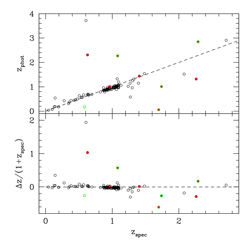
Figure 6.— Comparison of our photometric redshifts to 119 spectroscopic redshifts in the UDS field (top panel) and fractional error (bottom panel). Red filled circles denote those points flagged as QSOs in the Simpson et al. (2006) sample, and green open circles are objects with $\log(\chi^{2})>2.9$ as derived by EAZY.

This process was repeated for one of the lowest–sensitivity regions in the mosaic, the area of a single WFCAM chip in the northwest quadrant of the image. Even in this worst case the catalog is 100% complete for $K<23.2$ and 95% complete for $K\lesssim 23.5$ (see Figure 5). It should be noted that these completeness estimates are entirely based on point sources; for real galaxies with extended flux distributions, the completeness at a given magnitude will be lower. However, for the relatively bright galaxies considered in this analysis ($K<22.4$, or 1 magnitude brighter than the worst–case 95% completeness limit), this should not be an issue. Also, this does not take into account the possibility of close pairs of objects being blended, and thus mistakenly being counted as a single object by SExtractor; however, for this analysis such effects are likely to be small (further discussed in §8).

4.6. Catalog format

The final $K$–selected catalog employed in this analysis was generated from the 99022 objects (not lying near bad pixels) detected by SExtractor in the UDS mosaic. Some of these may be image artifacts and/or fall on bad or missing regions in the SXDS and SWIRE images as described in §4.3. Such objects are included in the catalog, but with flag(s) noting that their photometry in a given band is likely to be unreliable. Photometry in the $B$ through IRAC 4.5 $\mu$m bands, as well as limited morphological information, are included, and all fluxes are given with an AB zeropoint of 25. The columns of the catalog are as follows:

Columns (1)–(3).—Running ID, right ascension, and declination (J2000)
Columns (4)–(15).—$BRi^{\prime}z^{\prime}JK$ “color” fluxes and errors (1$\farcs$75 diameter aperture, listed in the order $f_{B}$, $\sigma_{B}$, $f_{R}$, $\sigma_{R}$, …)
Column (16).—Total $K$ flux in the SExtractor AUTO aperture
Columns (17)–(20).—IRAC 3.6$\mu$m and 4.5$\mu$m fluxes and errors (matched to the optical/IR “color” aperture)
Columns (21)–(23).—$K$–band half–light radius, ellipticity, and position angle
Columns (24)–(25).—Optical and SWIRE bad–pixel flags
Column (26).—Flag for objects not detected in the stacked $B+R+i^{\prime}+z^{\prime}$ image
Column (27).—Internal flag generated by SExtractor

5. Photometric Redshifts and rest–frame colors

5.1. EAZY fitting

Photometric redshifts were determined with the EAZY code, described in detail in Brammer et al. (2008). In its default configuration, EAZY uses $\chi^{2}$ minimization to fit linear combinations of six basis templates to broadband galaxy spectral energy distributions; a $K-$band luminosity prior and estimates of systematic errors due to template mismatch are also taken into account. These default settings have been demonstrated to provide reliable photometric redshifts for other $K$–selected samples (see Brammer et al., 2008).

To test the reliability of the UDS $z_{\rm phot}$ values we compared them to galaxies in this field with known spectroscopic redshifts. A query using the NASA Extragalactic Database (NED) finds 96 published redshifts, most of which are old passively–evolving galaxies at $0.8<z<1.2$ from Yamada et al. (2005). An additional 60 redshifts of radio sources are from the catalog of Simpson et al. (2006). After cross–correlating these objects with objects detected in the UDS $K$ band, 119 spectroscopic redshifts remained; EAZY was able to find $z_{\rm phot}$ solutions for 110 of these (and found no $\chi^{2}$ minimum for the other 9). The left–hand panel of Figure 6 shows a comparison of the photometric and spectroscopic redshifts of these galaxies. Objects flagged by Simpson et al. (2006) as “QSO” or “XQSO” (X-ray emitting QSO), which may not be well–fit by typical galaxy templates if the AGN light contributes significantly to the overall flux, are shown as filled red circles in the plot. Of the aforementioned nine objects for which EAZY failed to find $z_{\rm phot}$ solutions, four of them fell in this AGN category.

While the agreement between the photometric and spectroscopic redshifts is quite good (particularly at $z\sim 1$), roughly 8% of the points are outliers with fractional errors of 0.2 or more (and about half of these in turn are serious outliers, with $\left|\Delta z\right|/(1+z_{\rm spec})>0.5$). Determining a priori from photometry alone which objects are likely to be outliers is difficult – although most of the QSOs are indeed strong outliers, weak (or even strong) AGN activity in galaxies is not always evident. However, the $\chi^{2}$ value returned by EAZY appears to be a somewhat reliable indicator: all objects with $\log\chi^{2}>2.9$ have $(1+z_{\rm phot})$ values that deviate more than 20% from their measured spectroscopic redshifts. When objects with these high $\chi^{2}$ values are removed from the sample, the remaining normalized median absolute deviation (NMAD) in $\Delta z/(1+z_{\rm spec})$ is 0.033 with a median offset of $\Delta z=-0.013$.

At $z\sim 1.2$ the photometric redshifts appear to exhibit a small systematic offset of $\Delta z/(1+z)\sim-0.05$ (though due to the small number of points here it is difficult to assess the magnitude of the offset). A similar offset at the same redshift is seen by Brammer et al. (2008) even with more photometric bands included (notably $U$, $V$, and $H$), and the offset persists when different template sets and input parameters are used. Additionally, relatively small–scale “spikes” and “voids” (on the scale of $\Delta z=0.1-0.2$) in the photometric redshift distribution are apparent–see Figure 7. These may in part represent real variations in the large–scale galaxy distribution, but some are also likely to be numerical artifacts intrinsic to the photometric redshifts. However, since these effects are relatively small, and since in our analysis we employ redshift intervals ($\Delta z>0.5$) larger than the observed “spikes” in the $z_{\rm phot}$ distribution, such effects are not likely to significantly affect our results.

Figure 7.— Distribution of apparent $K$ magnitude as a function of photometric redshift (top panel), and number of galaxies as a function of $z_{\rm phot}$ (bottom panel).

The rest–frame near– and mid–infrared properties of typical galaxies are not as well constrained as the optical SEDs, so the galaxy templates employed by EAZY tend to be uncertain in this regime. This uncertainty is taken into account during the $z_{\rm phot}$ calculations; nevertheless, the inclusion of the IRAC data could still in principle introduce systematic effects. To check this, we re–ran EAZY with only the $BRi^{\prime}z^{\prime}JK$ photometry and compared the results to those with the IRAC fluxes included. While the resulting $z_{\rm phot}$ values were similar, the scatter and systematic offset increased substantially, with ${\rm NMAD}\left[\Delta z/(1+z_{\rm spec})\right]=0.044$ and median $\Delta z=-0.017$. Moreover, although the number of major outliers is comparable, such outliers are no longer easily rejected: even with the $\chi^{2}$ cut and excluding objects where solutions were not found, only three of the AGNs are excluded, and overall the worst outliers are no longer confined to the fits with the highest $\chi^{2}$ values.

Including IRAC data in the calculation of photometric redshifts thus reduces the $z_{\rm phot}$ scatter and allows outlying points (including many AGNs) to be rejected from the sample . This is perhaps not surprising: for example, Stern et al. (2005) find that AGNs typically have redder IRAC $[3.6]-[4.5]$ colors than typical galaxies. Since the galaxy templates employed by EAZY do not take possible AGN components into account, the 4.5 $\mu$m excess in galaxies with nuclear activity in turn cannot be matched well by any of these templates. Indeed, most of the objects that either had high $\chi^{2}$ values or no solutions from EAZY appeared to exhibit redder $[3.6]-[4.5]$ colors than those galaxies with good $z_{\rm phot}$ fits.

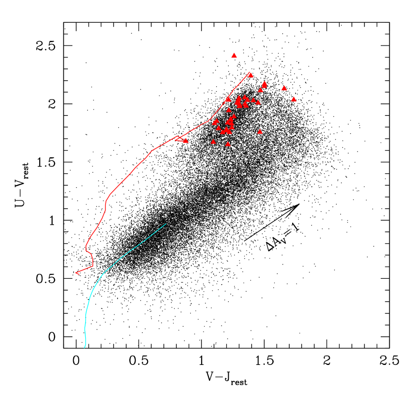
Figure 8.— Rest–frame color–color diagram for $K_{\rm AB}<22.4$, $z_{\rm phot}<2.5$ UDS galaxies (black points). Red points denote spectroscopically–confirmed $z\sim 1$ old passively–evolving galaxies (OPEGs) from Yamada et al. (2005) with little or no detected line emission ($W_{\lambda}({\rm OII})<5$ Å). Bruzual & Charlot (2003) evolutionary tracks of passively–evolving (red line) and constantly star–forming (cyan line) stellar populations from $0.1-10$ Gyr are overplotted, and the arrow shows the effect of 1 magnitude of dust extinction. The extended star–forming track and the “quiescent clump” (which overlaps with the OPEG sample) are clearly separated.

5.2. Monte Carlo analysis

During the process of computing $z_{\rm phot}$ values, EAZY also provides estimates on the redshift uncertainty and a probability distribution $p(z)$ for each object. The $p(z)$ curves in particular are useful for estimating the redshift distribution of a large sample of objects, since the true distribution is likely to be broader than a histogram of the best–fit $z_{\rm phot}$ values (e.g., in an extreme case with a sample of $z_{\rm phot}=2.00$ galaxies, the true distribution would be much broader than a delta function). To assess the consistency of the $p(z)$ distributions, we performed 120 Monte Carlo iterations varying the input photometry assuming Gaussian errors. Though this is a relatively small number of iterations, it gives a rough estimate of the $z_{\rm phot}$ uncertainty for any given object, and an accurate computation of the redshift distribution of a large sample of objects.

For each object, the median and dispersion among the 120 Monte Carlo runs were determined and compared to the estimates from EAZY. The median values for the UDS sample were consistent with the best–fit values derived by EAZY from the original (unperturbed) catalog, as were the $1\sigma$ uncertainty estimates. Furthermore, for subsets of the catalog, the redshift distributions derived from the Monte Carlo analysis closely reflected the EAZY–derived $p(z)$ distributions. The uncertainties derived by EAZY thus appear to be internally consistent for the UDS data.

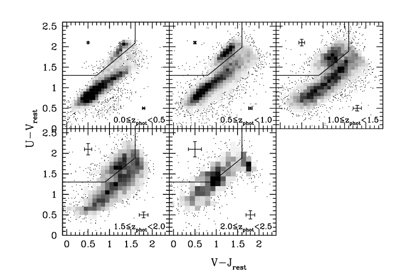
Figure 9.— Rest–frame $U-V$ vs. $V-J$ colors of UDS $K<22.4$ galaxies in five redshift bins. The greyscale represents the density of points in the central region of each plot, while outlying points are plotted individually. The solid lines show the adopted divisions between the star–forming and quiescent galaxy samples at each redshift, defined in Equation 4. Median uncertainties in the rest–frame colors of quiescent and star–forming galaxies (only taking random errors into account) are shown in the upper left and lower right of each frame, respectively.

5.3. Interpolating rest–frame photometry

At $z\sim 2.5$, the $U$, $V$, and $J$ rest–frame bands fall roughly into the observed $J$, $K$, and IRAC $4.5\mu$m bands respectively. Up to this redshift, intrinsic $UVJ$ fluxes can thus be interpolated from the observed data. Filter response curves for the observed bands, taking into account atmospheric absorption and detector quantum efficiency, were downloaded from each of the WFCAM, Suprime–Cam, and IRAC websites. For rest–frame filter definitions we used the standard filter definitions without atmospheric absorption or detector response included: the Bessell (1990) $U$ and $V$ curves, and the Mauna Kea definition (Tokunaga et al., 2002) for $J$. Rest–frame fluxes were then interpolated following the method of Rudnick et al. (2003). Uncertainties on the rest–frame fluxes were derived using the perturbed input catalogs and output redshifts from the Monte Carlo analysis described in §5.2. Note that these color uncertainties only take into account photometric errors (and the resulting $z_{\rm phot}$ errors), and do not include the uncertainties intrinsic to the templates used for $z_{\rm phot}$ fitting.

6. Evidence for quiescent galaxies to $z\sim 2.5$

6.1. The rest–frame colors of quiescent and star–forming galaxies

We use the galaxy catalog derived from the UDS/SXDS/SWIRE data, along with the photometric redshifts and interpolated rest–frame colors described in the previous section, to analyze the rest–frame color distribution of galaxies out to $z=2.5$. Beyond this redshift the rest–frame $J$ band begins to “fall off” the reddest filter in our catalog (IRAC $4.5\mu$m), and rest–frame colors at $z>2.5$ are therefore less reliable. Stars are selected (and removed from the sample) using the two criteria: $J-K<0$ and $(J-K)<0.2(i^{\prime}-K)-0.16$. This two–color cut was derived by inspection of the $J-K$ vs. $i^{\prime}-K$ color–color diagram, wherein stars form a tight, well–defined track. Additionally, we exclude all objects that fall on bad pixels or missing data regions in any band, as well as those with bad photometric redshift solutions ($\log\chi^{2}>2.9$ as derived in §5), and apply a magnitude limit of $K<22.4$. When all these criteria are met, the subsample analyzed hereafter contains 30108 galaxies between $0<z<2.5$. By comparison with 119 spectroscopic redshifts in the field we find typical photometric redshift errors of $\Delta z/(1+z)\sim 0.033$, though this is almost entirely measured with galaxies at $z\lesssim 1.2$; at higher redshifts the $z_{\rm phot}$ uncertainty is likely to be substantially larger.

Figure 8 shows the rest–frame $U-V$ vs. $V-J$ (hereafter $UVJ$) diagram for this subset of UDS galaxies. A striking bimodality emerges: one diagonal track extends from blue to red $V-J$, while a localized clump that is red in $U-V$ but blue in $V-J$ lies above this track. Previously, Labbé et al. (2005) and Wuyts et al. (2007) found that actively star–forming and quiescent galaxies segregate themselves in this plane, with the star–forming galaxies forming a diagonal track and quiescent galaxies populating mostly the upper left–hand region; with the far larger number of sources in the UDS, it is now evident that the galaxies form a truly bimodal distribution in this plane. Indeed, this interpretation is supported here by both data and models: the red points overlying the “quiescent clump” in Figure 8 are spectroscopically–confirmed old passively–evolving galaxies from Yamada et al. (2005), while the star–forming and quiescent loci are reasonably coincident with the corresponding Bruzual & Charlot (2003) stellar population models; a detailed analysis of the star–formation properties of galaxies in the $UVJ$ plane will be presented in a forthcoming paper (Labbé et al., in preparation).

Essentially, the $UVJ$ diagram allows the degeneracy between red star–forming and red quiescent galaxies to be broken: while galaxies with blue $U-V$ colors in general exhibit relatively unobscured star formation activity, red galaxies could be either quiescent galaxies with evolved stellar populations or dust–obscured starbursts. But since dust–free quiescent galaxies are blue in $V-J$, they occupy a locus in the $UVJ$ plane that is distinct from the star–forming galaxies, allowing the two populations to be empirically separated. Clearly, such a separation using a single color (such as $U-V$) would be fraught with problems: at best, the quiescent sample derived in this manner would be contaminated by red starbursts, and if the number of such starbursts were sufficiently high the bimodality would no longer be visible (see also Figure 10). Note that although the $U-B$ color is better at distinguishing between a narrow break (characteristic of an old stellar population) and broader dust reddening when spectroscopic redshifts are available, the larger uncertainties on photometric redshifts do not allow sufficiently accurate $U-B$ colors to be estimated.

Even when photometric redshifts are derived using alternative template sets within EAZY, or an entirely different $z_{\rm phot}$ code (HYPERZ; Bolzonella, Miralles, & Pelló, 2000), the basic bimodal shape of Figure 8 persists, indicating that this method is robust to the specific numerical technique employed.

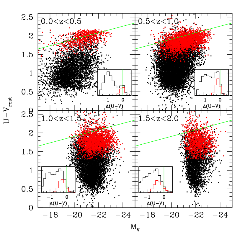
Figure 10.— Left panel: Number of red galaxies as a function of the normal distance from the diagonal dividing lines shown in Figure 9; the normal distance is defined such that, in these histograms, star–forming galaxies are to the left (i.e. negative values) and quiescent galaxies are on the right. Bimodality along this diagonal line is clearly evident up to $z=2$. Right panel: Color–magnitude diagrams in the same bins; red and black points denote quiescent and star–forming galaxies (selected on the basis of the cuts in Figure 9) respectively. The green line is a fit to the red points in the $0.0<z<0.5$ bin, and the inset plots show galaxy counts as a function of the distance in $U-V$ from this line (with quiescent galaxies plotted separately as a red histogram). Note that no $U-V$ bimodality is evident at $z>1.5$, even though it is clearly seen in the $UVJ$ plane.

6.2. Color Evolution

Changes in rest–frame colors with redshift reflect the intrinsic evolution of stellar populations, since all spectra have in principle been transformed to the same reference frame (barring possible $z_{\rm phot}$ systematic errors). $UVJ$ diagrams at five different redshifts (in bins of width $\Delta z_{\rm phot}=0.5$) are shown in Figure 9. The most immediately apparent feature is that the observed bimodal distribution of star–forming and quiescent galaxies is clearly seen up to $z\sim 2$. Although the scatter increases substantially at higher redshifts (to the point where it likely washes out any intrinsic bimodality at $z>2$), most likely due to a combination of larger photometric redshift uncertainties and weaker observed fluxes, the two distinct populations are nonetheless visible.

It is also notable that the shape of the star–forming sequence appears to change: at the lowest redshifts the sequence curves, but this may be due to the effects of using a small aperture on relatively nearby galaxies (i.e., the outermost, bluer parts of galaxies with large angular sizes falling outside the “color” aperture). At $z\gtrsim 0.5$, where the angular size–redshift relation begins to flatten, the dust sequence indeed becomes more linear. The increase in star formation activity at higher redshifts is also apparent in two ways: the fractional number of dusty, star–forming galaxies (the upper–right portion of the dust sequence) increases, and the entire dust sequence appears to move to redder $V-J$ colors. Note that at $2.0<z_{\rm phot}<2.5$ a concentration at red $V-J$ and $U-V$ appears; this mainly comprises galaxies with a substantial contribution from the red $A_{V}=2.75$ template included with EAZY. This single template substantially improves the $z_{\rm phot}$ solutions of very dusty galaxies, but can lead to the observed discrete clump in color–color space.

With increasing redshift the dead clump appears to steadily move to bluer $U-V$ (with the median $U-V$ changing by $\sim 0.15$ magnitudes between the $z=0-0.5$ and $z=1.5-2$ bins), while the $V-J$ color remains more or less unchanged. This is expected from passive evolution of the stellar populations in the clump, but relatively small systematic errors in the photometric redshifts (on the order of $\Delta z/(1+z)\sim 0.05$) can produce similar offsets in the average $U-V$ color of quiescent galaxies at $z\sim 1.5$. The $z_{\rm phot}$ estimates show a systematic offset that is smaller than this, about $(z_{\rm phot}-z_{\rm spec})/(1+z_{\rm spec})\sim-0.01$ over the full redshift range (see Figure 6). Nonetheless, given the lack of spectroscopic redshifts at $z\gtrsim 1.3$, we cannot ascertain whether there are larger systematic offsets at higher redshift, and therefore cannot accurately measure the color evolution of galaxies in the quiescent clump or absolutely define the boundaries of the box in which they live.

6.3. Sample Division

Since the color bimodality is visible up to $z\sim 2$, we employ empirical criteria to divide this sample into quiescent and star–forming subsamples. In each redshift bin of Figure 9 where the bimodality could be seen, an initial diagonal cut was first made between the two populations. Histograms of red galaxy counts relative to this line were then derived. The position of the diagonal cut was fine–tuned (keeping the same slope at all redshifts) to fall roughly between the two peaks (except in the lowest–redshift bin, where the shapes of the quiescent and star–forming galaxy loci made this impossible); Figure 10 (left panel) shows these histograms along the adjusted diagonal lines.

The adopted diagonal selection criteria for quiescent galaxies between $0<z<2.0$ bin are:

$$\begin{array}[]{lcccr}(U-V)>0.88\times(V-J)+0.69&&&&\left[0.0<z<0.5\right]\\ (U-V)>0.88\times(V-J)+0.59&&&&\left[0.5<z<1.0\right]\\ (U-V)>0.88\times(V-J)+0.49&&&&\left[1.0<z<2.0\right]\end{array}$$ (4)

Additional criteria of $U-V>1.3$ and $V-J<1.6$ are applied to the quiescent galaxies at all redshifts to prevent contamination from unobscured and dusty star–forming galaxies, respectively. The samples of star–forming galaxies are then defined by everything falling outside this box (but within the color range plotted in Figure 9, such that the very small number of extreme color outliers are not included in either sample). The two distinct populations are no longer visible at $z_{\rm phot}>2.0$, but the same dividing line used at $z=1-2$ is shown for reference. Note that the exact placement of this division does not significantly affect the results presented herein (see also §7 for a more detailed discussion). Typical random color uncertainties for the star–forming and quiescent samples at each redshift interval are shown in the lower right and upper left corners, respectively, of each panel in Figure 9.

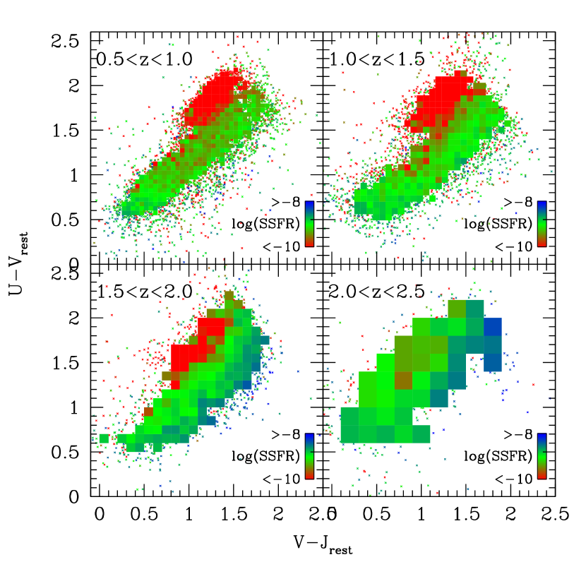
Figure 11.— Rest frame $UVJ$ diagram in four redshift ranges with bins color coded by the median specific star–formation rate of the galaxies within each bin; outliers in the $UVJ$ plane are plotted individually. The $z<0.5$ bin is not included here because the adopted SSFR proxies are not reliable at low redshifts. Quiescent galaxies lie in approximately the same region at all redshifts.

6.4. MIPS $24\mu$m measurements

Between $z\sim 1-2.5$, the $24\mu$m flux of galaxies is strongly correlated with dust–obscured star formation due to the presence of redshifted $6-12\mu$m polycyclic aromatic hydrocarbon (PAH) features in this band (Yan et al., 2004, e.g.). The observed $24\mu$m fluxes of the UDS galaxies can thus be used to empirically confirm whether the $UVJ$ criteria indeed select star–forming and quiescent galaxies. Since the $K$ band, which at these redshifts corresponds to rest–frame optical/NIR light, is a rough tracer of stellar mass, the $24\mu$m/$K$ flux ratio then provides an estimate of the dust–obscured specific star–formation rate (SSFR). Likewise, the UV–to–$K$ flux ratio provides an approximate measure of the unobscured SSFR, and thus the combination of these three bands provides a reasonably robust estimate of total SSFR.

Using the FIREWORKS catalog of Wuyts et al. (2008) we derive proxies for the IR and UV SSFR based on UV/$K$ and $24\mu m/K$ flux ratios, and use these proxies to obtain order–of–magnitude estimates of the SSFRs of UDS galaxies; the details of this derivation are given in the Appendix. Figure 11 shows the $UVJ$ diagram in four redshift bins between $0.5<z<2.5$ (the bin at $z<0.5$ is not shown, since the SSFR proxies are not expected to be effective at such low redshifts). Since the $24\mu$m data are too shallow for most galaxies in this sample to be detected individually, we combine the SSFRs of multiple galaxies as a function of $UVJ$ color as follows: at each redshift galaxies are divided into square $UVJ$ color bins. If $>10$ objects fall into a given bin, a square is plotted with a color corresponding to the median SSFR of the underlying galaxies (in essence “binning” the galaxies’ SSFR estimates); otherwise, individual points are plotted. A strong trend is clearly seen from $z=0.5-2$: the “quiescent clump” on average exhibits low SSFR, and is distinctly offset from the adjacent red star–forming galaxies.

In the $2.0<z<2.5$ bin of Figure 9 the scatter in the $UVJ$ diagram is too large for any intrinsic bimodality to be seen, and the trend in SSFR also appears weaker (Figure 11), perhaps due in part to the smaller number of points at high redshift and passive evolution. At $z>2$, we employ another approach to verify the presence of galaxies with relatively low SFRs: the top panel of Figure 12 again shows the $z=2-2.5$ $UVJ$ plot, with red galaxies selected by the rectangular boxes shown. The median $24\mu$m flux of the $N$ galaxies within each box, measured in 8″ diameter apertures, is then calculated. To estimate the uncertainties in the median fluxes, $N$ apertures were placed randomly on the MIPS image and the median $24\mu$m flux within these apertures calculated. This was repeated 500 times for each value of $N$, and the clipped standard deviation of these 500 trials was taken as the uncertainty in the median of the galaxy fluxes for every bin of $N$ galaxies. Note that since the randomly–placed apertures may contain bright and/or confusing $24\mu$m sources, this error estimate inherently takes both background and confusion noise into account.

Figure 12.— Rest–frame colors of bright ($K<22.4$), $2.0<z<2.5$ galaxies (top panel). Red galaxies with $1.3<(U-V)<2.0$ are selected by the boxes shown, and the median $24\mu$m MIPS flux for the galaxies within each box is plotted in the lower panel. The $24\mu$m flux rises at red $V-J$, confirming the trend suggested in the corresponding panel of Figure 11.

The median $24\mu$m fluxes within each bin are shown in the lower panel of Figure 12; indeed, $24\mu$m flux increases strongly with $V-J$ color, indicating that $V-J$ does indeed provide a good proxy for star formation rate at $z=2-2.5$ (with a factor of $\sim 5$ difference in $24\mu$m flux between the bluest and reddest galaxies in $V-J$). The trends in $24\mu$m flux and SSFR strongly suggest that the $UVJ$ selection criteria indeed separate quiescent from star–forming galaxies (even given the limited number of photometric bands available in UDS) at $z<2$, and may work reasonably well up to higher redshifts, $z\lesssim 2.5$. Since the color bimodality can no longer be seen at $z>2$ it is possible that the quiescent galaxy sample at these redshifts contains somewhat more contamination from red, star–forming galaxies; furthermore, the rest–frame $J$ flux estimate relies on the relatively shallow $3.6/4.5\mu$m data at $z>2$, which may result in subtle incompleteness effects in the sample at these redshifts. Therefore, for the remainder of our analysis we focus only on galaxies at $z<2$ where the bimodality can obviously be seen. It is also important to note that the presence of AGN may produce enhanced $24\mu$m emission and redder $V-J$ colors, and thus mimic the photometric effects of star formation. As described in §5, most objects with known strong AGN activity do not have valid $z_{\rm phot}$ solutions and have likely been removed from the sample; even so, some weak AGN activity may remain and contribute to the observed correlation.

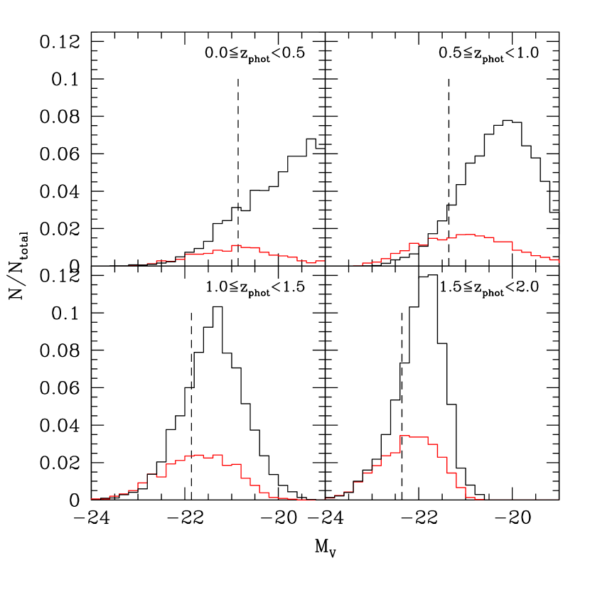
Figure 13.— Rest–frame $V$ magnitude distributions of the quiescent (red histogram) and star–forming (black histogram) galaxies in the four redshift ranges shown in Figure 10. The vertical dashed line shows the value of $M_{V}^{\star}$ at the central redshift of each bin, assuming the $z=0.1$ SDSS value of Blanton et al. (2003) and evolving as $M_{V}^{\star}(z)=M_{V}^{\star}(0)-z$. At high redshifts, quiescent galaxies compose roughly half of the total bright galaxy population, and a larger fraction at lower redshifts.

6.5. Luminosities

Absolute rest–frame $V$ magnitude histograms of the number counts of quiescent and star–forming galaxies in each redshift interval are shown in Figure 13. The value of $M_{V}^{\star}$ at the center of each redshift bin, assuming the Blanton et al. (2003) SDSS value at $z=0.1$ and evolving as $M_{V}^{\star}(z)=M_{V}^{\star}(0)-z$, is also shown. At bright magnitudes ($M_{V}\lesssim-22.5$) between $z\sim 1-2$, quiescent galaxies contribute approximately as much to the galaxy number density as those that are actively star–forming. This is similar to the result of Kriek et al. (2006), who found star formation rates consistent with zero in 9/20 bright galaxies at $z=2.0-2.7$, though their spectroscopic determination of SFRs is likely to produce fundamentally different “quiescent” samples than our rest–frame color definition. At lower redshifts ($0.5<z<1.0$), the luminous galaxy population is comprised of an larger fraction of quiescent galaxies, while galaxies with fainter $V$ luminosities (and hence which typically have lower stellar masses) are dominated by those undergoing star formation.

7. Clustering of quiescent and star–forming galaxies

To investigate the relation between halo mass and star formation activity at $z>1$, we calculate the clustering of the star–forming and quiescent galaxies (as defined by their rest–frame $UVJ$ colors) at these redshifts following the method of Quadri et al. (2007a, 2008); a brief summary of this method follows. The angular correlation function of each sample was computed using the Landy & Szalay (1993) estimator, taking into account all “bad” data regions (described in detail in §4.3). Figure 14 shows these functions for the quiescent and star–forming samples, with the former clearly exhibiting stronger clustering (in angular space) than the latter.

Because of the large number of objects in this catalog at $z=1-2$, it is possible to further break each of the quiescent and star–forming samples into bright and faint subsamples, thereby also investigating the effect of luminosity on clustering strength. Angular correlation functions were recomputed for star–forming and quiescent galaxies within two luminosity bins divided at $M_{V}=-22.0$. This is approximately the minimum luminosity at which the $z=1-2$ sample is complete—essentially all galaxies with $M_{V}<-22$ at $z=2$ have observed $K$ fluxes brighter than the $K<22.4$ cutoff, while at $M_{V}>-22$ some galaxies (most of which are low–mass and blue) fall below the $K$ flux limit. However, this should not affect the reliability of the $r_{0}$ determination itself since the Monte Carlo $z_{\rm phot}$ simulations (§5.2) fully account for differences in the redshift distributions. For each subsample we fit power laws to the angular correlation functions over the range $60\arcsec-300\arcsec$, and estimated $r_{0}$ using the Limber projection (see Quadri et al., 2007a, for details). The lower cutoff ensures that we are only measuring the large–scale correlation function, and are not unduly influenced by the clustering of galaxies within individual halos. The upper cutoff was chosen to minimize the importance of the integral constraint correction (see Quadri et al., 2008). The slope of the spatial correlation function is fixed to 1.6, which is consistent with each of the subsamples studied here, and the uncertainties are estimated using bootstrap resampling.

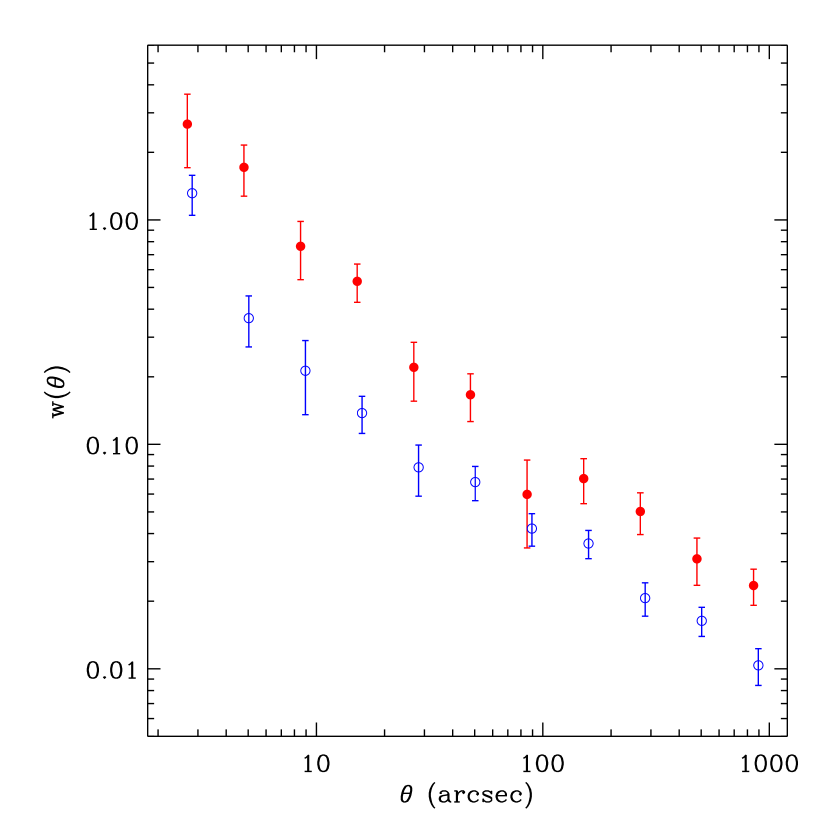
Figure 14.— Angular correlation functions for the $1.0<z_{\rm phot}<2.0$ quiescent (red filled circles and errorbars) and star–forming (blue open circles ) samples. The quiescent galaxy sample shows significantly stronger angular clustering.

The resulting clustering lengths of the quiescent and star–forming samples in both luminosity bins are shown in Figure 15. The clustering of bright quiescent galaxies is stronger (at $1.4\sigma$ significance) than that of the bright star–forming sample, with $r_{0}=9.5^{+1.1}_{-1.2}$ h^-1 Mpc and $7.4\pm 0.9$ h^-1 Mpc respectively, and the difference in clustering length becomes far more pronounced in the fainter bin. Interestingly, the clustering length of quiescent galaxies appears to be independent of luminosity; star–forming galaxies, on the other hand, exhibit a marginal increase in clustering strength with luminosity. The stronger clustering of bright galaxies in the combined (star–forming plus quiescent) sample thus appears to be driven by both the larger quiescent fraction among bright galaxies as well as the stronger clustering of star–forming galaxies.

The exact criteria used to divide the “quiescent” and “star–forming” samples (i.e. the lines shown in Figure 9) may have an effect on this result. While we chose the diagonal dividing line to lie centered between the star–forming track and quiescent “clump,” this is not necessarily the best criterion. For example, moving the line “upward” (toward redder $U-V$ and bluer $V-J$) would result in a less complete sample of quiescent galaxies that is also less contaminated by star–forming galaxies scattering across the line; similarly, moving the line down toward the star–forming track increases completeness at the expense of contamination. To check whether this affects the clustering measurement, we moved the diagonal divider by $0.1$ magnitudes in both directions and re–calculated the $r_{0}$ values. The perturbed $r_{0}$ values were all within $1\sigma$ of the old values, with one exception: when the dividing line was moved upwards (i.e. defining a less complete quiescent galaxy sample with less contamination), the clustering strength of bright ($M_{V}<-22$) quiescent galaxies increased by $\sim 1.5\sigma$. Therefore, the result that quiescent galaxies exhibit a larger clustering length appears robust to the color criteria used to select the quiescent sample.

The clustering length we have found for quiescent galaxies at $z=1-2$ is fully consistent with the value of $r_{0}=10.6\pm 1.6h^{-1}$ Mpc for $z_{\rm phot}=2-3$ DRGs in this catalog (Quadri et al., 2008). This is perhaps not surprising, as roughly half of the $z_{\rm phot}>2$ DRGs in this sample fall within the “quiescent” $UVJ$ selection region.

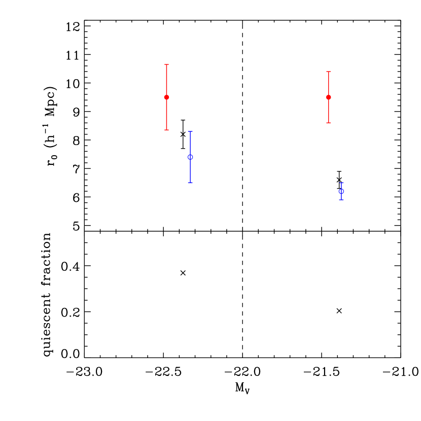
Figure 15.— Deprojected real–space clustering length in two absolute magnitude bins ($M_{V}<-22$ and $M_{V}>-22$) for the $1.0<z_{\rm phot}<2.0$ quiescent (red filled circles and errorbars), star–forming (blue open circles), and combined (black crosses) galaxy samples. For each point, the median $M_{V}$ of the corresponding sample is plotted. The lower panel shows the fraction of quiescent galaxies in each bin. Quiescent galaxies exhibit stronger clustering, and thus occupy more massive dark matter halos, than star–forming galaxies in both magnitude bins.

8. Discussion

The presence of a bimodal population of galaxies in the $UVJ$ plane to at least $z\sim 2$ is consistent with previous spectroscopic studies, such as Kriek et al. (2008b), who find a nascent red sequence at $z\sim 2.3$. The purely photometric analysis presented herein allows much larger samples of quiescent galaxies to be found, albeit with lower confidence for any individual object. At first glance, however, this appears to be in conflict with the Cirasuolo et al. (2007) claim that the galaxy bimodality disappears at $z\sim 1.25-1.5$. In fact, the apparent discrepancy between these results is probably due to observational effects: Cirasuolo et al. (2007) consider only bimodality in the rest–frame color–magnitude ($U-B$ vs. $M_{B}$) diagram, i.e. the “red sequence” method. Indeed, as the right panel of Figure 10 shows, such a plot does not show a bimodal population of galaxies at $z_{\rm phot}>1.5$, even though the bimodality is still present in the $UVJ$ diagram. Similarly, the absence of a bimodal distribution in the $UVJ$ diagram at $z>2$ (Figure 10, left panel) does not necessarily imply the disappearance of bimodality in the underlying galaxy population, but rather reflects the larger photometric and $z_{\rm phot}$ uncertainties at these redshifts (as can also be seen from the large $UVJ$ error bars at $2<z_{\rm phot}<2.5$; Figure 9).

Using a single rest–frame color (determined via photometric redshifts) to select quiescent and star–forming galaxies can obscure an underlying bimodality for two reasons: (1) the population of dusty, star–forming galaxies increases with redshift, and these have significant overlap their optical colors with any red, quiescent galaxies that may be present; and (2) the greater scatter in the rest–frame $U-V$ or $U-B$ at higher redshifts can effectively wash out the intrinsic red sequence. This increased scatter is due not only to the larger uncertainties on measured photometry of fainter galaxies at large redshift, but also the larger photometric redshift uncertainties (Kriek et al., 2008a). As previously mentioned, $U-B$ by itself is only effective at distinguishing quiescent from dusty galaxies when accurate spectroscopic redshifts are available; with photometric redshifts the rest–frame color uncertainty is too large to see the quiescent red sequence. The use of $V-J$ in addition to $U-V$ helps mitigate both of these problems: $V-J$ separates red, quiescent galaxies from red, dust–obscured starbursts (Figure 8), and a two–dimensional color bimodality is more resilient to increased scatter than a single color. Thus, when only photometric redshifts are available, the two–color $UVJ$ technique employed herein appears to provide a “cleaner” selection of high–redshift, quiescent galaxies than standard red–sequence methods.

The differences between high–redshift quiescent and star–forming galaxy properties can provide clues to the physical mechanisms behind star formation (or the lack thereof). In the moderately high–redshift ($z=1-2$) sample considered here, the most striking contrasts between the two populations are in their clustering strengths and luminosities. Quiescent galaxies cluster more strongly than those undergoing active star formation (implying, from standard CDM theory, that they reside preferentially in higher–mass halos) and typically exhibit brighter absolute $V$ magnitudes, comprising about half of the bright galaxy population at all redshifts. However, the clustering strength of quiescent galaxies does not appear to be strongly dependent on luminosity: as shown in Figure 15, the bright and faint quiescent samples exhibit roughly equal clustering lengths, which in turn are consistently higher than the corresponding values for star–forming galaxies. This may be indicative of a characteristic halo mass above which star formation is inhibited.

Our results may be taken to suggest that the star formation-density relation was already in place at $z\sim 1.5$, with quiescent galaxies more strongly clustered and hence situated, on average, in denser regions. On first glance this would seem to contradict recent claims of a “reversal” of the star formation–density relation that occurs at $z\sim 1-1.5$ (e.g. Elbaz et al., 2007; Cooper et al., 2008). These authors present evidence that the average SFR per galaxy in dense regions is higher than in less dense regions, in contrast to the well–known relationship in the local universe. Whether this constitutes a “reversal” is in part a matter of terminology; it may be true that the typical star formation rate increases with environmental density (as found by, e.g., Cooper et al., 2008), but this does not preclude the possibility that the relatively rare quiescent galaxies are preferentially found in the densest regions (as suggested by our results). We also note that the star formation–density relation may be qualitatively different depending on whether one is considering absolute star formation rates or specific star formation rates (see Cooper et al., 2008).

The observed segregation of quiescent and star–forming galaxies both in clustering strength and luminosity suggests strong links between halo mass, stellar mass, and the cessation of star formation. Different theoretical bases for the quenching of star formation in galaxies hosted by massive halos have been proposed, some focusing on radio–mode AGN feedback processes which prevent further gas cooling and star formation (e.g. Croton et al., 2006; Bower et al., 2006, and references therein), while others suggest that hot accretion and shock processes in high–mass halos may be sufficient to produce quiescent galaxies without invoking AGN (Keres et al., 2005; Birnboim, Dekel, & Neistein, 2007). Although these models may not represent the definitive explanation for the observational results presented here, the correspondence between theory and observation is nonetheless intriguing. Further observations of large quiescent galaxy samples (e.g., comparing the radio emission of high–$z$ quiescent and star–forming galaxies) are likely to shed further light on the underlying quenching mechanism.

9. Caveats

This analysis employs photometric redshifts, which of course are much less well–constrained than those determined using spectroscopy. Furthermore, the number of spectroscopic redshifts for comparison is quite small, with 119 available spec–$z$s in this field. Essentially all of these known redshifts are from two samples, neither of which can be considered unbiased: a set of $z\sim 1$ old passively–evolving galaxies, and galaxies selected from their radio emission (thus all likely exhibiting some degree of AGN activity). If anything, one might expect photometric redshift determinations to be worse in this latter sample since the templates used to derive the phot–$z$s do not include AGN activity; however, Figure 6 shows that the fits are actually quite good from about $z=0-1.5$ (and the worst outliers, including two–thirds those with signatures of AGN, are excluded through either a $\chi^{2}$ cut or the lack of a $z_{\rm phot}$ solution). The fit to the “old” $z\sim 1$ galaxy sample was even better, with fractional redshift errors on the order of 2%. At $z\gtrsim 1.5$ it is likely that these fractional errors are at least $\sim 0.07$, the scatter found in the EAZY–derived photometric redshifts from the CDFS–GOODS catalog (which included several more photometric bands than the UDS$+$SXDS$+$SWIRE dataset; Brammer et al., 2008).

It is nonetheless possible that some additional systematic errors remain in the photometric redshifts. Such errors would manifest themselves as shifts in the rest–frame colors, the magnitude of which primarily depend on the galaxy redshift and template shape. However, the results presented herein are not dependent on the exact rest–frame colors themselves, but rather on the relative separation between the quiescent and star–forming populations. Since the two populations are clearly visible from $z=0-2$ (Figure 9), and the positions of galaxies in the $UVJ$ plane are strongly correlated with $24\mu$m flux (Figure 11), we conclude that we can distinguish populations of galaxies based on their relative star–formation rates. It is nonetheless important to note that the absolute values of the interpolated rest–frame colors may still be subject to systematic, possibly redshift–dependent offsets, and these offsets may be different depending on the SED (e.g. for quiescent and star–forming galaxies). Further differences are likely to come about with differing photometric redshift codes and techniques for determining rest–frame colors. This underscores the importance of defining such empirical color cuts based on the actual data and analysis techniques employed; relying on criteria defined on other datasets can lead to inaccurate results.

Another possible source of error is the ability of SExtractor to deblend close pairs of objects. Where two extended sources overlap, or if the separation of two point sources is smaller than a few times the $K$–band PSF FWHM ($\sim$0$\farcs$7), oftentimes the two objects will be counted as a single object. In this case, the galaxy clustering is probably underestimated at the smallest scales ($<1.5$″ or so). Even if they are successfully identified as separate objects, the fixed color apertures used to measure fluxes are likely to be contaminated, and thus may cause errors in photometric redshifts and rest–frame colors. However, the fraction of objects in such close pairs is negligible compared to the total catalog. Furthermore, these clustering results are based on larger–scale correlations—i.e., we do not calculate the clustering below $\theta\sim 2\farcs$. Thus, this incompleteness at the smallest scales is unlikely to affect our results.

10. Conclusions

From our matched multiband UDS$+$SXDS$+$SWIRE $K$–selected catalog we have derived reliable photometric redshifts and rest–frame colors. For a relatively bright ($K<22.4$) subsample of this catalog, we find that:

1. Galaxies show strong bimodal behavior in rest–frame $U-V$ vs. $V-J$ color–color space, with one population of “dead” (non–star forming) galaxies, and a sequence of dusty, actively star–forming galaxies. This behavior can be seen out to $z\sim 2$, so the observed present–day galaxy bimodality was present at least to this redshift; however, at $z\gtrsim 1.5$ the bimodality is not seen in a single–color–magnitude diagram.

2. From $z=0$ to $2.5$, the rest–frame $V-J$ color (at red $U-V$ colors) shows a strong correlation with our estimates of specific star–formation rate, indicating that the $V-J$ color is a reliable tracer of star formation activity even at $z>2$ where the rest–frame color uncertainties are too large for the bimodality to be seen.

3. Quiescent and star–forming galaxies at $z>1$ contribute roughly equally to the overall galaxy population at the brightest $V$ luminosities; the less luminous population is dominated by actively star–forming objects.

4. The clustering strength of quiescent galaxies from $z=1-2$ appears to be independent of galaxy luminosity, and is consistently stronger than the clustering of the actively star–forming galaxies; thus, “dead” galaxies appear to occupy more massive halos than those which are in the process of forming stars. This suggests a link between halo mass and the early cessation of star formation activity.

Forthcoming data releases of the UKIDSS UDS, including deep $H$–band data and ultimately reaching a depth of $K=24.9$ (AB), will allow these results to be tested with even fainter, higher–redshift galaxies. More importantly, the 290–hour ultra–deep Spitzer legacy survey of the UDS field (SpUDS; PI: J. Dunlop) currently being undertaken will provide at least an order–of–magnitude increase in exposure time compared to the SWIRE data used in this paper, giving much–improved constraints on photometric redshifts, AGN activity, and rest–frame colors.

Appendix A Estimating specific star–formation rates

Accurately determining specific star formation rates (SSFR; i.e. SFR as a fraction of galaxy mass) typically requires deep UV and $24\mu$m data in order to measure unobscured and obscured star formation, respectively. Unfortunately, the UDS data presented here currently lack several key ingredients; i.e. there are no $U$-band data, the available SWIRE $24\mu$m data are shallow, and the necessary detailed models for determining galaxy masses and the $24\mu$m–$L_{IR}$ conversions are beyond the scope of this work. However, to test the validity of the $UVJ$ colors as a tracer of SSFR, such precision is not necessary: simple order–of–magnitude estimates will suffice.

Over the redshift range $0.5<z<2.5$, we therefore resort to a proxy based entirely on observed photometry and calibrated with the Chandra Deep Field–South FIREWORKS catalog of Wuyts et al. (2008). Reliable SSFRs were derived from FIREWORKS based on the rest–frame 2800Å luminosity and observed $24\mu$m fluxes (Wuyts et al., in preparation). The sum of these two contributions should then approximate the total amount of star formation in “typical” galaxies (i.e. those without extreme obscuration, like SMGs). Since $K$ flux is itself a tracer of stellar mass, it follows that the $f_{\rm UV}/f_{K}$ flux ratio (for some observed band that falls in or near the rest–frame ultraviolet) can provide a rough estimate of the unobscured SSFR, and $f_{24\mu m}/f_{K}$ should do the same for the “dusty” SSFR.

From the FIREWORKS data we find that a single linear relation sufficiently describes the correlation between the IR SSFR and $f_{24\mu m}/f_{K}$ over $0.5<z<2.5$. There is also a strong correlation between UV SSFR and $f_{R}/f_{K}$; however, the exact slope and normalization of the relation appear to change abruptly at $z\sim 1$; for the UV relation we thus perform separate linear fits at $0.5<z<1$ and $1<z<2.5$. This UV proxy is somewhat flatter (i.e. insensitive to $f_{R}/f_{K}$) than the $24\mu$m–SFR relation, and substantially underestimates the largest UV SSFRs by a factor of $\sim 2$, but it appears to accurately reproduce relatively low SSFRs ($la2\times 10^{9}$ yr^-1); thus, this UV proxy is effectively used as an additive term to correct the fluxes of galaxies which are faint in $24\mu$m. The best–fit relations, shown in Figure 16, are:

$$\begin{array}[]{l}{\rm SSFR}_{\rm IR}=-2.2\times 10^{-11}+1.85\times 10^{-10}(f_{24}/f_{K})\\ {\rm SSFR}_{\rm UV}(z<1)=-7.4\times 10^{-10}+3.8\times 10^{-9}(f_{R}/f_{K})\\ {\rm SSFR}_{\rm UV}(z>1)=-5.8\times 10^{-10}+5.8\times 10^{-9}(f_{R}/f_{K})\end{array}$$ (A1)

Note that the UV relations formally yield substantially negative SSFR values even when $f_{R}/f_{K}>0$, since SSFR_UV is not quite a linear function of $f_{R}/f_{K}$; thus, we require that the UV contribution to the total SSFR be positive (i.e. for any object where SSFR${}_{\rm UV}<0$, we set SSFR${}_{\rm UV}=0$). Since a large number of galaxies have $f_{24\mu m}<0$ due to background noise, and the SSFR_IR relation appears very close to linear, we do allow individual objects to have SSFR${}_{\rm IR}<0$ in the stacking analysis.

Figure 16.— Relations used to derive specific star–formation rates from the observed IR ($f_{\rm 24\mu m}/f_{K}$; top panel) and UV ($f_{R}/f_{K}$; bottom panel) flux ratios. Data in this figure are from the FIREWORKS catalog of Wuyts et al. (2008); the IR relation shown is fit to galaxies between $0.5<z<2.5$ and the UV at $1.0<z<2.5$ (a similar UV relation was derived for the $z=0.5-1$ galaxies, not shown here). The IR SSFR shows a good correlation with $f_{24\mu m}/f_{K}$ over the full range, but the UV relation tends to underestimate large SSFRs.

References

- Baldry et al. (2004) Baldry, I. K., Glazebrook, K., Brinkmann, J., Ivezić, Ž., Lupton, R .H., Nichol, R. C., & Szalay, A. S. 2004, ApJ, 600, 681
- Bertin & Arnouts (1996) Bertin, E., & Arnouts, S. 1996, A&AS, 117, 393
- Bertin et al. (2002) Bertin, E., Mellier, Y., Radovich, M., Missonnier, G., Didelon, P., & Morin, B. 2002, in ASP Conf. Ser. 281, Astronomical Data Analysis Software and Systems XI, ed. D. A. Bohlender, D. Durand, & T. H. Handley (San Francisco: ASP), 228
- Bessell (1990) Bessell, M. S. 1990, PASP, 102, 1181
- Birnboim, Dekel, & Neistein (2007) Birnboim, Y., Dekel, A., & Neistein, E. 2007, MNRAS, 380, 339
- Blanton et al. (2003) Blanton, M. R., et al. 2003, ApJ, 592, 819
- Bolzonella, Miralles, & Pelló (2000) Bolzonella, M., Miralles, J.-M., & Pelló, R. 2000, A&A, 363, 476
- Bower et al. (2006) Bower, R. G., et al. 2006, MNRAS, 370, 645
- Brammer et al. (2008) Brammer, G. B., van Dokkum, P. G., & Coppi, P. 2008, ApJ, 686, 1503
- Bruzual & Charlot (2003) Bruzual, G. & Charlot, S. 2003, MNRAS, 344, 1000
- Budavari et al. (2003) Budavári, T., et al. 2003, ApJ, 595, 59
- Casali et al. (2007) Casali, M., et al. 2007, A&A, 467, 777
- Cirasuolo et al. (2007) Cirasuolo, M., et al. 2007, MNRAS, 380, 585
- Cooper et al. (2008) Cooper, M. C., et al. 2008, MNRAS, 383, 1058
- Croton et al. (2006) Croton, D., et al. 2006, MNRAS, 365, 11
- Daddi et al. (2004) Daddi, E., et al. 2004, ApJ, 617, 746
- Daddi et al. (2005) Daddi, E., et al. 2005, ApJ, 626, 680
- Elbaz et al. (2007) Elbaz, D., et al. 2007, A&A, 468, 33
- Förster Schreiber et al. (2006) Förster Schreiber, N., et al. 2006, AJ, 131, 1891
- Franx et al. (2003) Franx, M., et al. 2003, ApJ, 587, L79
- Gawiser et al. (2006) Gawiser, E., et al. 2006, ApJS, 162, 1
- Giavalisco et al. (2004) Giavalisco, M., et al. 2004, ApJ, 600, L93
- Grazian et al. (2007) Grazian, A., et al. 2007, A&A, 465, 393
- Hambly et al. (2008) Hambly, N. C., et al. 2008, MNRAS, 384, 637
- Hewett et al. (2006) Hewett, P. C., Warren, S. J., Leggett, S. K., & Hodgkin, S. T. 2006, MNRAS, 367, 454
- Kauffmann et al. (2003) Kauffmann, G., et al. 2003, MNRAS, 341, 33
- Keres et al. (2005) Keres, D., Katz, N., Weinberg, D. H., & Davé, R. 2005, MNRAS, 363, 2
- Kriek et al. (2006) Kriek, M., et al. 2006, ApJ, 649, L71
- Kriek et al. (2008a) Kriek, M., et al. 2008, ApJ, 677, 219
- Kriek et al. (2008b) Kriek, M., et al. 2008, ApJ, 682, 896 (arXiv:0804.4175)
- Kron (1980) Kron, R. 1980, ApJ, 43, 305
- Labbé et al. (2003) Labbé, I., et al. 2003, AJ, 125, 1107
- Labbé et al. (2005) Labbé, I., et al. 2005, ApJ, 624, L81
- Labbé et al. (2006) Labbé, I., Bouwens, R., Illingworth, G. D., & Franx, M. 2006, ApJ, 649, L67
- Landy & Szalay (1993) Landy, S. D., & Szalay, A. S. 1993, ApJ, 412, 64
- Lawrence et al. (2007) Lawrence, A., et al. 2007, MNRAS, 379, 1599
- Lonsdale et al. (2003) Lonsdale, C. J., et al. 2003, PASP, 115, 897
- Miyazaki et al. (2002) Miyazaki, S., et al. 2002, PASJ, 54, 833
- Papovich et al. (2006) Papovich, C., et al. 2006, ApJ, 640, 92
- Quadri et al. (2007a) Quadri, R., et al. 2007a, ApJ, 654, 138
- Quadri et al. (2007b) Quadri, R., et al. 2007b, AJ, 134, 1103
- Quadri et al. (2008) Quadri, R., et al. 2008, ApJ, 685, 1
- Rudnick et al. (2003) Rudnick, G., et al. 2003, ApJ, 599, 847
- Rudnick et al. (2006) Rudnick, G., et al. 2006, ApJ, 650, 624
- Sekiguchi et al. (2004) Sekiguchi, K., et al. 2004, BAAS, 36, 1478
- Simpson et al. (2006) Simpson, C., et al. 2006, MNRAS, 372, 741
- Steidel et al. (1996) Steidel, C. C., Giavalisco, M., Pettini, M., Dickinson, M., Adelberger, K. L. 1996, ApJ, 462, L17
- Stern et al. (2005) Stern, D., et al. 2005, ApJ, 631, 163
- Tokunaga et al. (2002) Tokunaga, A. T., Simons, D. A., & Vacca, W. D. 2002, PASP, 114, 180
- van Dokkum et al. (2006) van Dokkum, P. G., et al. 2006, ApJ, 638, L59
- Warren et al. (2007a) Warren, S. J., et al. 2007, MNRAS, 375, 213
- Warren et al. (2007b) Warren, S. J., et al. 2007, preprint, arXiv:astro-ph/0703037
- Wuyts et al. (2007) Wuyts, S., et al. 2007, ApJ, 655, 51
- Wuyts et al. (2008) Wuyts, S., Labbé, I., Förster Schreiber, N., Franx, M., Rudnick, G., Brammer, G., & van Dokkum, P. 2008, ApJ, 682, 985
- Yamada et al. (2005) Yamada, T., et al. 2005, ApJ, 634, 861
- Yan et al. (2004) Yan, L., et al. 2004, ApJS, 154, 75