Gauge theory picture of an ordering transition in a dimer model

Abstract

We study a phase transition in a 3D lattice gauge theory, a ”coarse-grained” version of a classical dimer model. Duality arguments indicate that the dimer lattice theory should be dual to a XY model coupled to a gauge field with geometric frustration. The transition between a Coulomb phase with dipolar correlations and a long range ordered columnar phase is understood in terms of a Higgs mechanism. Monte Carlo simulations of the dual model indicate a continuous transition with exponents close but apparently different from those of the 3d XY model. The continuous nature of the transition is confirmed by a flowgram analysis.

Realizing that seemingly unrelated phenomena obey the same rules is certainly one of the most fascinating aspects of physics. In the context of phase transitions between different states of matter, this issue of universality is often addressed within Landau-Ginzburg-Wilson (LGW) theory, where one derives an action in powers of the order parameter describing a spontaneous symmetry breaking. Recently, new kinds of unconventional phase transitions which do not easily fit in the LGW framework have been discussed in the domain of strongly correlated systems. A first example is the quantum phase transition arising in some frustrated antiferromagnets from a Néel state with antiferromagnetic order (AF) to a valence bond solid (VBS) state which breaks lattice symmetries Senthil . Another case is the classical interacting dimer system on the cubic lattice Alet , which displays a continuous transition from an ordered phase where the dimers align in columns to a Coulomb phase with dipolar dimer correlations. In all cases, two important issues have to been considered: first, one has to make sure that the transition is indeed critical and not first-order. Then, one must seek for alternative (“non-LGW”) descriptions of the phase transition. For instance, the possibility of a continuous AF-VBS transition has been proposed to be understood in terms of spinon deconfinement Senthil . However, this deconfined quantum criticality scenario is confronted with recent simulations favoring a very weak first-order driven process Kuklovnew .

In this paper, we focus on the effective description of the phase transition in the classical dimer model. There, a gauge field arises naturally in the Coulomb phase HKMS ; Alet . One generally introduces the lattice electric field: $E_{i}(\textbf{r})=(-1)^{\textbf{r}}n_{i}(\textbf{r})$ with n being the dimer occupation number. To capture the hardcore nature of the dimers, a divergence constraint is obeyed: $\mathbf{\nabla}\cdot\textbf{E}=\pm 1$. In the Coulomb phase, the long wavelength properties of the system are described by the coarse-grained action: $S=\frac{K}{2}\int\textbf{E}^{2}\textrm{d}^{3}r$. Due to the energy form of the microscopic model, the dimer system is driven at low temperatures to a columnar phase with broken lattice symmetries. Using some duality transformations, we argue in this paper that this transition can be understood in terms of a Higgs mechanism. At the critical point, the system is described by a field theory closely linked to the one appearing in studies of deconfined quantum criticality. The same scenario has been recently proposed by mapping the classical dimer model to a quantum 2d bosonic model Powell2 . We study via Monte Carlo (MC) simulations the transition of the effective dual model between Coulomb and columnar phases to recover its continuous nature.

We start by considering a “coarse-grained” model where the electric field on the lattice can take all integer values, which generalizes the microscopic case. Nevertheless, we retain the divergence constraint $\mathbf{\nabla}\cdot\textbf{E}=\pm 1$. Our starting point is the following action on the lattice:

$$Z = \int_{-\pi}^{\pi}\left[D\theta\right]\sum_{E_{i}(\mathbf{r)}=-\infty}^{+\infty}e^{-S_{\mathrm{Coulomb}}-S_{\mathrm{const}}}$$

$$S_{\mathrm{Coulomb}} = \frac{J}{2}\sum_{\mathbf{r}}E_{i}^{2}\left(\mathbf{r}\right)$$

$$S_{\mathrm{cons}} = i\sum_{\mathbf{r}}\theta(\mathbf{r)}\left(\nabla_{i}E_{i}^{0}(\mathbf{r)}-\nabla_{i}E_{i}\left(\mathbf{r}\right)\right).$$

with $E_{i}^{0}(\mathbf{r)=}\frac{(-1)^{\mathbf{r}}}{6}e_{i}$ and the angular field $\theta$ is a Lagrange multiplier ensuring the divergence constraint. A real-valued field is then introduced via the Poisson formula:

$$\sum_{E_{i}(\mathbf{r})=-\infty}^{+\infty}e^{-S\left[E_{i}\left(\mathbf{r}\right)\right]}\rightarrow$$

$$\sum_{u_{i}\left(\mathbf{r}\right)=-\infty}^{+\infty}\int_{-\infty}^{+\infty}\left[D\mathbf{E}\right] \exp\left(-S\left[E_{i}\left(\mathbf{r}\right)\right]-\sum_{\mathbf{r}}2i\pi E_{i}u_{i}\left(\mathbf{r}\right)\right).$$

Performing a duality transformation Motrunich1 , we introduce the dual current $q_{i}=\epsilon_{ijk}\nabla_{j}u_{k}$ and the gauge field A defined by $\mathbf{B}=\frac{1}{2\pi}\epsilon_{ijk}\nabla_{j}A_{k}$ where $B_{i}=E_{i}-E_{i}^{0}$. We also define the static vector $\textbf{X}^{0}$ by $E_{i}^{0}=\frac{1}{2\pi}\epsilon_{ijk}\nabla_{j}X_{k}^{0}$. The circulation of $\textbf{X}^{0}$ is equal to $\frac{\pi}{3}$ modulo $2\pi$ on each dual plaquette. The dual theory corresponds now to a magnetic field coupled to the currents q with a static frustration field $\textbf{X}^{0}$. Adding a fugacity term for the currents: $S_{f}=\frac{1}{2\lambda_{m}}\sum(q_{i})^{2}$ , one can easily perform the integration over the q variables and find:

$$S\left[A_{i},\chi\right] = \frac{\mathcal{K}}{2}\sum_{\mathbf{r}^{\ast}}\left(\nabla_{i}A_{j}-\nabla_{j}A_{i}\right)^{2}$$ (1)

$$- \lambda_{m}\sum_{\mathbf{r}^{\ast}}\cos\left(\nabla_{k}\chi-A_{k}-X_{k}^{0}\right),$$

with the field $\chi$ resulting from the conservation of the dual currents. The different steps above were already discussed for related 3D quantum spin models Motrunich1 ; Motrunich2 . We are left with a dual theory of one matter field interacting with a non compact gauge field with geometric frustration. Note that the non-compactness of the field originates from the absence of monomers in the original dimer model. We can now discuss the possible phases encountered in this dual model. For small $\lambda_{m}$, the gauge field is essentially free and exhibits dipolar correlations. When $\lambda_{m}$ increases, the matter field condenses and gaps the gauge field by the Higgs mechanism. However, this condensation is constrained by the frustration vector $\textbf{X}^{0}$.

To find how the matter field condenses, one standard possibility Motrunich1 ; Motrunich2 ; Blankschtein et al. is to consider the soft spin version of Eq. 1. The kinetic energy turns out to have a two-dimensional manifold of minima, giving rise to an effective Ginzburg-Landau action function of the two complex matter fields $\mathbf{\phi}=\left(\phi_{1},\phi_{2}\right)$ Motrunich1 :

$$S=\int\textrm{d}^{3}r\left(|(\nabla_{i}-iA_{i}){\mathbf{\phi}}|^{2}+U(\phi)+\frac{K}{2}(\nabla\times\mathbf{A})^{2}\right),$$ (2)

with $U(\phi)=r|\mathbf{\phi}|^{2}+u|\mathbf{\phi}|^{4}+v_{8}I_{8}({\mathbf{\phi}})$ and where the exact form of the 8th order term $I_{8}$ has been derived in Ref. Motrunich1, for a quantum-mechanical model in $3+1$ dimensions.

The criticality of field theories such as Eq. 2 has been of great interest in recent years. In $(2+1)$ dimensions, it is in principle related to the AF-VBS transition at the deconfined quantum critical point Senthil , up to the $I_{8}$ term. The connection between the original dimer model and the effective action Eq. 2 was recently derived independently Powell2 . Note that the presence of the frustration vector $\textbf{X}^{0}$ in Eq. 1 is of crucial importance for the analysis above. The non-frustrated model, being dual to a XY theory, is known to present an inverted XY transition which therefore lies in the 3D XY universality class Dasgupta-Bartolomew . Its associated field theory corresponds to a single matter field interacting with a gauge field. We therefore expect a different behavior with and without frustration.

Theoretically, the $\epsilon$ expansion is of no help to characterize the transition as it predicts a first order transition Halperin-Lubensky for both one component and two component matter field model. Several high performance simulations Sudbofirst ; Kuklov on easy-plane lattice versions of two matter fields models have shown evidence for a weak first order transition, in contrast with the continuous transition predicted by the deconfined criticality scenario. Recent simulations on $SU(2)$ versions are controversial, with some pointing towards a continuous transition Motrunichnew while sophisticated analyses favor a first-order process Kuklovnew .

There are several caveats when considering the two-matter fields model. The first problem comes from the inherent approximations performed when taking the soft spin version of Eq. 1, and then going back to the lattice for the numerical simulations. Secondly, simulating Eq. 2 is more complicated than Eq. 1 as we have more degrees of freedom with the two-matter fields. Finally and most importantly, the connection is lost with the original dimer model, our main motivation. In some cases, it might be simpler to go one step back and simulate an intermediately-derived field theory such as Eq. 1, when available. This has the advantage of being at the same time closer to the microscopic dimer model (and therefore making it possible to use microscopic observables such as the columnar order parameter) as well as to a gauge-theory description (which is necessary to invoke the Higgs mechanism). In this paper, we adopt this strategy and present results of a MC simulation performed on Eq. 1 which shows a transition between a columnar and a dipolar phase. The transition is continuous with exponents found close but possibly different from those of the 3d XY universality class. We used the Metropolis algorithm on cubic lattices of size $L^{3}$ with periodic boundary conditions up to $L=64$, taking $\lambda_{m}=\beta=1/T$.

We first take $\mathcal{K}=1$ and present thermodynamic results. We checked that the probability distribution of the action reveals no double peak structure, supporting the scenario of a second order transition. The second moment of the action $M_{2}=\langle\left(S-\langle S\rangle\right)^{2}\rangle/L^{2}$ displays a peak at the transition point (see Fig. 1a). The height of the peak grows slowly up to $L=32$ and then converges within error bars for larger systems. The critical temperature $T_{c}^{M_{2}}=1.05(1)$ is estimated from the position of the maximum. The fact that $M_{2}$ converges at the transition indicates a critical exponent $\alpha$ negative, as in the 3d XY universality class. We note that $M_{2}$ appears to converge more rapidly with system size than for the non-frustrated model (data not shown), similar to the situation found in Ref. Motrunichnew, . This suggests an exponent $\alpha$ larger (in absolute value) than for the 3d XY universality class although it is difficult to give a precise value.

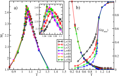
Figure 1: (color online) a) Second moment $M_{2}$ versus $T$ for different system sizes. Inset: Zoom on the peak. b) Columnar order parameter $C$ and transverse magnetic field correlator $G(\textbf{p}_{\mathrm{min}})$ as a function of $T$ for different system sizes.

We now consider the low-temperature phase. In this lattice gauge theory, a gauge-invariant order parameter related to lattice symmetry breaking can be defined. In the original microscopic model, dimers order on columns as temperature is lowered. Equivalently in the coarse grained model, the magnetic field B arranges in staggered flux lines in one particular direction. We therefore define the local order parameter $c_{i}(\textbf{r})=(-1)^{\textbf{r}-r_{i}}B_{i}(\textbf{r})$ and the associated global parameter:

$$C=\frac{1}{L^{3}}\|\textbf{C}\|=\frac{1}{L^{3}}\|\sum_{\textbf{r}}\textbf{c}(\textbf{r})\|.$$

At low $T$, we expect one of the component of the vector C to be non-zero, resulting in a finite expectation value. The original columnar states of the dimer model are represented by the configurations with: $\vec{C}=\left\{\pm C,0,0\right\},\left\{0,\pm C,0\right\},\left\{0,0,\pm C\right\}$. In Fig. 1b, $C$ is observed to vanish at high T, to take a non-zero value as $T$ decreases and to finally behave as $1/T$ at low $T$ as can be understood from the equations of motion. To locate the critical point, we measure the Binder cumulant of the order parameter $B=\langle C^{4}\rangle/\langle C^{2}\rangle^{2}$, which admits a crossing point for different systems sizes (see Fig. 2). This is characteristic of a second order transition and leads to an estimate $T_{c}^{col}=1.044(5)$. Assuming the standard scaling form $B=f(L^{1/\nu}(T-T_{c}))$, the derivative $dB/dT$ should scale as $L^{1/\nu}$ at criticality. We have measured this quantity thermodynamically, and display its scaling in the left inset of Fig. 2 for the temperatures $T=1.04$ and $T=1.05$ around the estimated $T_{c}$. Fits to a power-law form at these two $T$ allow to bound $0.70<\nu<0.82$. The other inset shows the best data collapse of the curves according to the scaling form with $\nu=0.73$ and $T_{c}=1.044$. We find that acceptable data collapses can also be obtained for values in the rather broad range $\nu=0.65-0.85$.

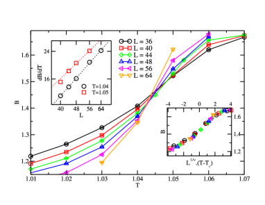
Figure 2: (color online) Binder cumulant of the columnar parameter versus $T$. Left inset: Divergence of the derivative $dB/dT$ close to $T_{c}$ versus system size (log-log scale). Right inset: Binder cumulant scaling collapse.

To characterize the high $T$ phase and detect its Coulomb nature, we study the evolution of the transverse magnetic field correlator at small momentum Olsson ; Kajantie : $G(\textbf{p}_{\mathrm{min}})=\frac{1}{L^{3}}\langle\hat{B}_{i}(\textbf{p}_{\mathrm{min}})\hat{B}_{i}(-\textbf{p}_{\mathrm{min}})\rangle$ with $\hat{B}_{i}(\textbf{p})$ the Fourier transform of $B_{i}(\textbf{r})$ and $\textbf{p}_{\mathrm{min}}=2\pi\hat{x}/L$. $G(\textbf{p}_{\mathrm{min}})=1$ if the gauge field presents dipolar correlations and $G(\textbf{p}_{\mathrm{min}})\to 0$ if the field has short range correlations. In our case, we expect the field to acquire a mass in the low-T phase as the matter field condenses. The evolution of $G(\textbf{p}_{\mathrm{min}})$ with $T$ is shown in Fig. 1 b. At high $T$, $G(\textbf{p}_{\mathrm{min}})\to 1$ and the gauge field is gapless. As $T$ is lowered, $G(\textbf{p}_{\mathrm{min}})$ decreases and the field becomes massive due to the Higgs mechanism. Close to the critical point, we assume the following scaling ansatz: $L^{\eta_{A}}.G(\textbf{p}_{\mathrm{min}})=f(L^{1/\nu}(T-T_{c}))$, where gauge and scale invariance impose $\eta_{A}=1$ at the critical point Tesanovic-Calan . The crossing of $L.G$ for different system sizes at $T_{c}$ has been observed in the non-frustrated model, leading to an estimate $\nu=0.67$ Olsson . The frustrated model also presents a crossing point (see Fig. 3) at $T_{c}^{G}=1.035(5)$. The scaling versus $L$ of the numerical derivative $LdG/dT$ leads to an independent estimate $\nu=0.73(5)$ (see left inset of Fig. 3), agreeing with the less precise values obtained from the Binder cumulant. The value of $\alpha$ obtained with hyperscaling $\alpha=2-\nu d$ agrees with the convergence of $M_{2}$. The data collapse of $L.G$ obtained with this value of $\nu$ is also of good quality (see right inset).

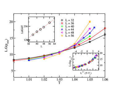
Figure 3: (color online) $L.G$ versus $T$ for different system sizes. Left inset: Scaling of the derivative $LdG/dT$ versus system size $L$ (log-log scale). Right inset: Data collapse of $L.G$.

So far, if the transition looks well continuous, we cannot totally exclude a very weak first-order process, with a very large but finite correlation length. In order to confirm this, we change the value of the stiffness $\mathcal{K}$ and implement the flowgram method Kuklov ; Kuklovnew . This method relies on the demonstration that the large scale behavior for a large value of $\mathcal{K}$ is identical to that at a smaller value of $\mathcal{K}$ where the nature of the transition can be easily determined. For each $\mathcal{K}$, we follow Ref. Motrunichnew, and define the operational critical temperature $T_{c}(L)$ for a size $L$ as the temperature where the Binder ratio is equal to $B_{c}=1.41$ noteBC . We then compute for each value of $\mathcal{K}$ and $L$ the value of $L.G$ and recover the flows. If all the curves within an interval $\mathcal{K}\in[\mathcal{K}_{1},\mathcal{K}_{2}]$ can be collapsed into a single master curve by rescaling the system size, then it implies that the order of the transition remains the same within the interval. A diverging flow for the collapse is a clear sign of a first order transition. We present here the flowgram obtained for our model with $\mathcal{K}\in[0.36,2.2]$ on Fig  4. We have succeeded in performing a collapse of the curves by rescaling $L\rightarrow C(\mathcal{K})L$ with $C(\mathcal{K})=2.0/\mathcal{K}+0.4/\mathcal{K}^{2}$. The collapse is clearly converging. This suggests that scale invariance is reached and goes in favor of a continuous transition in the interval considered, confirming the previous analysis at $\mathcal{K}=1$.

To summarize our results, we have shown how, via a duality transformation, the interacting dimer model on the cubic lattice can be understood in terms of a complex matter field coupled to a gauge field with geometric frustration. As for the microscopic dimer model Alet , we found a direct continuous transition (by the Higgs mechanism) between a dipolar Coulomb phase at low coupling and a columnar phase which breaks lattice symmetries at high coupling. However, critical exponents are rather different from the ones obtained in the original dimer model (where $\alpha\simeq 0.5$ and $\nu\simeq 0.5$). In particular, the second moment of the action clearly shows no diverging peak in our case. The anomalous dimension $\eta_{A}$ is in agreement with the scale dimension of the stiffness in Ref. Alet, but a different value of $\nu$ is obtained.

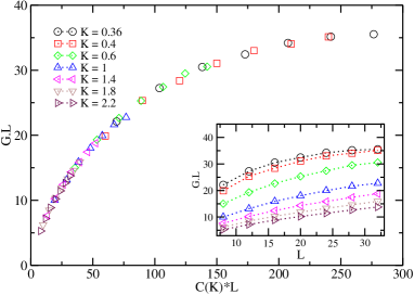
Figure 4: (color online) Data collapse of the Flowgram of the model. Inset: flows for different values of $\mathcal{K}$, note how the flows look more convergent for smaller stiffness.

The exponents that we find ($\nu\simeq 0.73$ and $\alpha<0$) seem to be slightly different from those of the 3d XY universality class (and consequently of the non-frustrated version of Eq. 1), although we cannot exclude it within our numerical accuracy. In both cases, we are left with an interesting open problem as there is no field theoretical arguments allowing to say that we should end up in the XY universality class. In view of our original motivation, an intriguing possibility remains that the microscopic dimer model is directly self-tuned (for unknown reasons) to a tricritical point. The flowgram analysis displays no sign of tricriticality however in the range of stiffness considered. Since values of $\mathcal{K}<0.36$ cannot be reached as the critical temperature is too low for the Metropolis algorithm to be efficient, one alternative would be to directly perturb the original microscopic dimer model to check this scenario.

We thank F. Delduc, I. Herbut, A. Honecker, G. Misguich, V. Pasquier and A. Vishwanath for enlightening discussions, and GENCI for allocation of CPU time. Simulations used the ALPS libraries ALPS .

References

- (1) T. Senthil et al., Science, 303, 1490 (2004); Phys. Rev. B 70, 144407 (2004)
- (2) F. Alet et al., Phys. Rev. Lett. 97, 030403 (2006); G. Misguich, V. Pasquier and F. Alet, Phys. Rev. B 78, 100402(R) (2008)
- (3) A.B. Kuklov et al., Phys. Rev. Lett. 101, 050405 (2008); preprint arXiv:0805.2578
- (4) D.A. Huse et al., Phys. Rev. Lett. 91, 167004 (2003)
- (5) S. Powell and J.T. Chalker, preprint arXiv:0805.3968; see also Phys. Rev. B 78, 024422 (2008)
- (6) O.I. Motrunich and T. Senthil, Phys. Rev. B 71, 125102 (2005)
- (7) K. Gregor and O.I. Motrunich Phys. Rev. B 76, 174404 (2007). See also D.L. Bergman, G.A. Fiete and L. Balents, ibid. 73, 134402 (2006).
- (8) D. Blankschtein, M. Ma and A.N. Berker, Phys. Rev. B 30, 1362 (1984); R.A. Jalabert and S. Sachdev, ibid. 44, 686 (1991); C. Lannert, M.P.A. Fisher and T. Senthil, ibid. 63, 134510 (2001)
- (9) C. Dasgupta and B.I. Halperin, Phys. Rev. Lett. 47, 1556 (1981); J. Bartholomew, Phys. Rev. B 28, 5378 (1983)
- (10) B.I. Halperin, T.C. Lubensky and S. Ma, Phys. Rev. Lett. 32, 292 (1974); J.H. Chen, T.C. Lubensky and D.R. Nelson, Phys. Rev. B 17, 4274 (1978)
- (11) A.B. Kuklov et al., Ann. Phys. 321, 1602 (2006)
- (12) S. Kragset et al., Phys. Rev. Lett. 97, 247201 (2006)
- (13) O.I. Motrunich and A. Vishwanath, preprint arXiv:0805.1494
- (14) K. Kajantie et al., Nucl. Phys. B 699, 632 (2004)
- (15) P. Olsson and S. Teitel, Phys. Rev. Lett. 80, 1964 (1998)
- (16) I.F. Herbut and Z. Tesanović, Phys. Rev. Lett. 76, 4588 (1996); C. de Calan and F.S. Nogueira, Phys. Rev. B 60, 4255 (1999)
- (17) We checked that the results hold if is slightly varied.
- (18) F. Albuquerque et al., J. Magn. Magn. Mater. 310, 1187 (2007); M. Troyer, B. Ammon and E. Heeb, Lect. Notes Comput. Sci., 1505, 191 (1998). See http://alps.comp-phys.org.