AGN Dusty Tori: I. Handling of Clumpy Media

Abstract

According to unified schemes of Active Galactic Nuclei (AGN), the central engine is surrounded by dusty, optically thick clouds in a toroidal structure. We have recently developed a formalism that for the first time takes proper account of the clumpy nature of the AGN torus. We now provide a detailed report of our findings in a two-paper series. Here we present our general formalism for radiative transfer in clumpy media and construct its building blocks for the AGN problem — the source functions of individual dusty clouds heated by the AGN radiation field. We show that a fundamental difference from smooth density distributions is that in a clumpy medium, a large range of dust temperatures coexist at the same distance from the radiation central source. This distinct property explains the low dust temperatures found close to the nucleus of NGC1068 in 10 $\mu$m interferometric observations. We find that irrespective of the overall geometry, a clumpy dust distribution shows only moderate variation in its spectral energy distribution, and the 10$\mu$m absorption feature is never deep. Furthermore, the X-ray attenuating column density is widely scattered around the column density that characterizes the IR emission. All of these properties are characteristic of AGN observations. The assembly of clouds into AGN tori and comparison with observations is presented in the companion paper.

1. INTRODUCTION

Although there are numerous AGN classes, a unified scheme has been emerging steadily (e.g., Antonucci, 1993, 2002; Urry & Padovani, 1995). The nuclear activity is powered by a supermassive black hole and its accretion disk, and this central engine is surrounded by a dusty toroidal structure. Much of the observed diversity is simply explained as the result of viewing this axisymmetric geometry from different angles. The torus provides anisotropic obscuration of the central region so that sources viewed face-on are recognized as “type 1”, those observed edge-on are “type 2”. From basic considerations, Krolik & Begelman (1988) conclude that the torus is likely to consist of a large number of individually very optically thick dusty clouds. Indeed, Tristram et al. (2007) find that their VLTI interferometic observations of the Circinus AGN “provide strong evidence for a clumpy or filamentary dust structure”. A fundamental difference between clumpy and smooth density distributions is that radiation can propagate freely between different regions of an optically thick medium when it is clumpy, but not otherwise. However, because of the difficulties in handling clumpy media, models of the torus IR emission, beginning with Pier & Krolik (1992), utilized smooth density distributions instead. Rowan-Robinson (1995) noted the importance of incorporating clumpiness for realistic modeling, but did not offer a formalism for handling clumpy media.

We have recently developed such a formalism and presented initial reports of our modeling of AGN clumpy tori in Nenkova, Ivezić, & Elitzur (2002), Elitzur, Nenkova, & Ivezić (2004), and Elitzur (2006, 2007). We now offer a detailed exposition of our formalism and its application to AGN observations. Because of the wealth of details, the presentation is broken into two parts. In this paper we describe the clumpiness formalism and construct the source functions for the emission from individual optically thick dusty clouds, the building blocks of the AGN torus. In a companion paper (Nenkova et al., 2008, part II hereafter) we present the assembly of these building blocks into a torus and the application to AGN observations.

2. CLUMPY MEDIA

We start by presenting a general formalism for handling clumpy media. For completeness, the full formalism is described here, including results that are utilized only in part II.

Consider a region where the matter is concentrated in clouds (see Fig. 1). For simplicity we take all clouds to be identical; generalizing our results to a mixture of cloud properties is straightforward (Conway, Elitzur, & Parra, 2005). Individual clouds are characterized by their size $R_{\rm c}$, the cloud distribution is specified by the number of clouds per unit volume $n_{\rm C}$. Denote by $V_{\rm c}$ the volume of a single cloud and by $\phi$ the volume filling factor of all clouds, i.e., the fraction of the overall volume that they occupy. We consider the medium to be clumpy whenever

$$\phi=\hbox{$n_{\rm C}$}\hbox{$V_{\rm c}$}\ll 1\,.$$ (1)

In contrast, the matter distribution is smooth, or continuous, when $\phi\simeq 1$. It is useful to introduce the number of clouds per unit length

$$\hbox{$N_{\rm C}$}=\hbox{$n_{\rm C}$}\hbox{$A_{\rm c}$}=\ell^{-1}$$ (2)

where $A_{\rm c}$ is the cloud cross-sectional area and $\ell$ is the photon mean free path for travel between clouds (Fig. 1). Since $\hbox{$V_{\rm c}$}\simeq\hbox{$A_{\rm c}$}\hbox{$R_{\rm c}$}$, the clumpiness condition (eq. 1) is equivalent to

$$\phi=\hbox{$N_{\rm C}$}\hbox{$R_{\rm c}$}\ll 1,\qquad\hbox{or}\quad\hbox{$R_{\rm c}$}\ll\ell.$$ (3)

The clumpiness criterion is met when the mean free path between clouds greatly exceeds the cloud size.

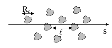
Figure 1.— A region populated by clouds of size $R_{\rm c}$. Along ray $s$, the photon mean-free-path is $\ell$ and the number of clouds per unit length is $N_{\rm C}$ = $\ell^{-1}$.

2.1. Emission from a clumpy medium

When the clumpiness criterion is met, each cloud can be considered a “mega-particle”, a point source of intensity $S_{\rm c,\lambda}$ and optical depth $\tau_{\lambda}$. The intensity at an arbitrary point $s$ along a given path can then be calculated by applying the formal solution of radiative transfer to the clumpy medium. The intensity generated in segment $ds^{\prime}$ around a previous point $s^{\prime}$ along the path is $\hbox{$S_{\rm c,\lambda}$}(s^{\prime})\hbox{$N_{\rm C}$}(s^{\prime})ds^{\prime}$. Denote by $\hbox{$\cal N$}(s^{\prime},s)=\int_{s^{\prime}}^{s}\hbox{$N_{\rm C}$}ds$ the mean number of clouds between $s^{\prime}$ and $s$ and by $\hbox{$P_{\rm esc}$}(s^{\prime},s)$ the probability that the radiation from $s^{\prime}$ will reach $s$ without absorption by intervening clouds. Natta & Panagia (1984) show that when the number of clouds is distributed around the mean $\hbox{$\cal N$}(s^{\prime},s)$ according to Poisson statistics,

$$\hbox{$P_{\rm esc}$}(s^{\prime},s)=e^{-t_{\lambda}(s^{\prime},s)},\qquad\hbox{where}\quad t_{\lambda}(s^{\prime},s)=\hbox{$\cal N$}(s^{\prime},s)(1-e^{-\tau_{\lambda}});$$ (4)

the Appendix discusses the validity of the Poisson distribution and presents the derivation of this result. Its intuitive meaning is straightforward in two limiting cases. When $\tau_{\lambda}<1$ we have $t_{\lambda}(s^{\prime},s)\simeq\hbox{$\cal N$}(s^{\prime},s)\tau_{\lambda}$, the overall optical depth between points $s^{\prime}$ and $s$; that is, clumpiness is irrelevant when individual clouds are optically thin, and the region can be handled with the smooth-density approach. It is important to note that $\hbox{$\cal N$}\tau_{\lambda}$ can be large—the only requirement for this limit is that each cloud be optically thin. The opposite limit $\tau_{\lambda}>1$ gives $\hbox{$P_{\rm esc}$}(s^{\prime},s)\simeq e^{-{\cal N}(s^{\prime},s)}$. Even though each cloud is optically thick, a photon can still travel between two points along the path if it avoids all the clouds in between.

With this result, the intensity at $s$ generated by clouds along the given ray is

$$\hbox{$I^{\rm C}_{\lambda}$}(s)=\int^{s}e^{-t_{\lambda}(s^{\prime},s)}\hbox{$S_{\rm c,\lambda}$}(s^{\prime})\hbox{$N_{\rm C}$}(s^{\prime})ds^{\prime}$$ (5)

This relation is the exact analog of the formal solution of standard radiative transfer in continuous media, to which it reverts when the cloud sizes are decreased to the point that they become microscopic particles; in that case $\tau\ll 1$ for each particle and $\ell^{-1}$ is the standard absorption coefficient. The only difference between the clumpy and continuous cases is that optical depth is replaced by its effective equivalent $t_{\lambda}$ and absorption coefficient is replaced by the number of clouds per unit length $N_{\rm C}$. It should be noted that, because of the particulate composition of matter, the solution of radiative transfer is always valid only in a statistical sense, corresponding in principle to the intensity averaged along the same path over an ensemble of many sources with identical average properties. However, in the smooth-density case the large number of dust particles along any path (a column with unity optical depth contains $\sim$ $10^{10}$ particles when made up of 0.1 $\mu$m dust grains) implies such small relative fluctuations around the mean that the statistical nature can be ignored and the results considered deterministic. For example, the intensity contours produced by a smooth-density spherical distribution are perfectly circular for all practical purposes. In the clumpy case, on the other hand, the small number of particles along the path can lead to substantial deviations from the mean intensity $I^{\rm C}_{\lambda}$. In contrast with the smooth density case, the intensity of a spherical cloud distribution can fluctuate significantly around concentric circles even though the distribution average properties are constant on such circles. The flux emitted from the enclosed circular area involves areal integration which smoothes out and reduces these fluctuations, so deviations of individual spectral energy distributions (SED) from their average are expected to be smaller than the brightness fluctuations. In general, the SED can be expected to have lower fluctuations than the brightness in clumpy distributions with a smoothly behaved function $N_{\rm C}$. Estimating fluctuations is beyond the scope of our formalism, which is predicated on averages at the outset. An assessment of fluctuations would require an extended theoretical apparatus or analysis of Monte-Carlo simulations, such as those described by Hönig et al. (2006).

After characterizing the clumpy medium by the cloud size $R_{\rm c}$ and the volume density of clouds $n_{\rm C}$ we introduced an equivalent set of two other independent variables—the volume filling factor $\phi$ and the number of clouds per unit length $N_{\rm C}$. Our final expression for the intensity does not involve $\phi$; only $N_{\rm C}$ enters. A complete formalism that would not invoke the assumption $\phi\ll 1$ would lead to a series expansion in powers of $\phi$, and the expression we derived in eq. 5 is the zeroth order term in that expansion. In fact, detailed Monte Carlo simulations show that, to within a few percents, this expression describes adequately clumpy media with $\phi$ as large as 0.1 (Conway, Elitzur & Parra, in preparation). Since the intensity calculations are independent of the volume filling factor, their results do not provide any information on this quantity, nor do they provide separate information on either $R_{\rm c}$ or $n_{\rm C}$, only on $N_{\rm C}$. In complete analogy, the radiative transfer problem for smooth density distributions does not involve separately the size of the dust grains or their volume density, only the combination $n_{\rm d}\sigma_{\rm d}$, which determines the absorption coefficient and which is equivalent to $N_{\rm C}$.

Equation 5 accounts only for the radiation generated along the path by the clouds themselves. A path containing a background source, such as the line of sight to the AGN, requires different handling since averaging is then meaningless. For such a line of sight, the intensity $I_{k}$ generated when there are exactly $k$ intervening clouds ($k=0,1,2,\dots$) has a Poisson probability $P_{k}$. The only meaningful quantities that can be deduced from modeling in this case are tabulations of the intensities $I_{k}$ and their associated probabilities $P_{k}$; that is, the probability is $P_{0}$ that the intensity is $I_{0}$ (the unobscured AGN), $P_{1}$ that it is $I_{1}$, etc. An actual source will correspond to one particular member of this probability distribution.

2.2. The cloud distribution

The only distribution required for intensity calculation is $N_{\rm C}$, the number of clouds per unit length. Our interest is primarily in cloud distributions with axial symmetry in which $N_{\rm C}$ depends only on the distance $r$ from the distribution center and the angle $\beta$ from the equatorial plane (the complementary of the standard polar angle). The total number of clouds along radial rays slanted at angle $\beta$ is, on average, $\hbox{${\cal N}_{\rm T}$}(\beta)=\int\!\hbox{$N_{\rm C}$}(r,\beta)\,dr$. It is convenient to introduce as a free parameter the mean of the total number of clouds along radial rays in the equatorial plane, ${\cal N}_{0}$ = ${\cal N}_{\rm T}$(0). The angular profile $\hbox{${\cal N}_{\rm T}$}(\beta)/\hbox{${\cal N}_{0}$}$ is expected to decline as $\beta$ increases away from the equatorial plane in AGN tori.

2.3. Total mass in clouds

The mass of a single cloud can be written as $\simeq\hbox{$m_{\rm H}$}N_{\rm c,H}\hbox{$A_{\rm c}$}$, where $N_{\rm c,H}$ denotes column density and $m_{\rm H}$ is the hydrogen nucleus mass. With the aid of eq. 2 and introducing the distribution profile $\hbox{$\eta_{\rm C}$}(r,\beta)=(1/\hbox{${\cal N}_{0}$})\hbox{$N_{\rm C}$}(r,\beta)$, the total mass in clouds is

$$M_{\rm C}=\hbox{$m_{\rm H}$}N_{\rm c,H}\hbox{${\cal N}_{0}$}\int\!\!\hbox{$\eta_{\rm C}$}\,dV$$ (6)

where the integration is over the entire volume populated by clouds. Note that $N_{\rm c,H}\hbox{${\cal N}_{0}$}$ is the mean overall column density in the equatorial plane. The total mass of a smooth distribution with the same equatorial column density would be given by the same expression except that the profile $\eta_{\rm C}$ would then describe the normalized gas density distribution.

The result in equation 6 for the overall mass in the clouds is independent of the filling factor $\phi$. The only property of an individual cloud that enters into this expression is its column density $N_{\rm c,H}$, which is directly related to its optical depth. The cloud size $R_{\rm c}$ is irrelevant so long as it meets the clumpiness criterion eq. 3.

2.4. Total number of clouds

Similar to the intensity, the overall mass involves the number of clouds per unit length $N_{\rm C}$, not the cloud volume density $n_{\rm C}$. The latter quantity enters in the calculation of the total number of clouds $n_{\rm tot}=\int\hbox{$n_{\rm C}$}dV$. Expressing $n_{\rm tot}$ too in terms of $N_{\rm C}$ brings in the cloud size because $n_{\rm tot}=\int(\hbox{$N_{\rm C}$}/\hbox{$A_{\rm c}$})dV$. With $\hbox{$A_{\rm c}$}\simeq R_{\rm c}^{2}$ and $\hbox{$R_{\rm c}$}=\phi/\hbox{$N_{\rm C}$}$,

$$n_{\rm tot}=\hbox{$\cal N$}_{0}^{3}\int{\eta_{\rm c}^{3}\over\phi^{2}}\,dV.$$ (7)

Among the quantities of interest, $n_{\rm tot}$ is the only one dependent upon the volume filling factor. Self-consistency of our formalism requires $\phi\ll 1$ to ensure the clumpiness criterion and $n_{\rm tot}\gg\hbox{${\cal N}_{0}$}$ to validate the Poisson distribution along paths through the source (see Appendix). Since $\eta_{\rm C}$ obeys the normalization $\int\!\hbox{$\eta_{\rm C}$}(r,0)\,dr=1$, $n_{\rm tot}$ is of order $\sim$ $\hbox{$\cal N$}_{0}^{3}/\phi^{2}$ and the two requirements are mutually consistent.

2.5. Covering Factors

Various AGN studies have invoked the concept of a “covering factor” in different contexts. The covering factor is generally understood as the fraction of the sky at the AGN center covered by obscuring material. This is the same as the fraction of randomly distributed observers whose view to the center is blocked. Therefore the average covering factor of a random sample of AGN is the same as the fraction, $f_{2}$, of type 2 sources in this sample; that is, $f_{2}$ is the average of the fraction of the AGN radiation absorbed by obscuring clouds. Denote the spectral shape of the AGN radiation by $f_{\rm e\lambda}$, normalized according to $\int\hbox{$f_{\rm e\lambda}$}d\lambda=1$. The fraction of the AGN luminosity escaping through a spherical shell of radius $r$ centered on the nucleus is, on average,

$$\hbox{$p_{\rm AGN}$}(r)=\int_{0}^{1}\!\!d\sin\beta\int\!d\lambda\,\hbox{$f_{\rm e\lambda}$}\,P_{\lambda,\rm esc}(r,\beta)\,,$$ (8)

where $P_{\lambda,\rm esc}(r,\beta)$ is the probability for a photon of wavelength $\lambda$ emitted by the AGN in direction $\beta$ to reach radius $r$ (eq. 4). Therefore $f_{2}=1-\hbox{$p_{\rm AGN}$}(R_{\rm out})$, where $R_{\rm out}$ is the torus outer radius, a relation that holds independent of the magnitude of the optical depth of individual clouds. The spectral integration involves all wavelengths in general, and is limited to the relevant spectral range in cases of specific obscuring bands. When the clouds are optically thick to the bulk of the AGN radiation, $P_{\lambda,\rm esc}(R_{\rm out},\beta)\simeq e^{-{\cal N}_{\rm T}(\beta)}$, independent of $\lambda$ (eq. 4). Utilizing the normalization of $f_{\rm e\lambda}$ then yields

$$f_{2}=1-\int_{0}^{\pi/2}e^{-{\cal N_{\rm T}}(\beta)}\cos\beta d\beta.$$ (9)

In a recent study Maiolino et al. (2007) defined the “dust covering factor” as the ratio of thermal infrared emission to the primary AGN radiation. Since the bulk of the AGN output is in the optical/UV, the radiation absorbed by the torus clouds must be re-radiated in infrared, therefore this dust covering factor is the fraction $f_{2}$ for optical/UV. In X-rays, the fraction $f_{2}$ is usually derived from the statistics of sources that have at least one obscuring cloud, whether Compton-thick or not, along the line of sight to the AGN. Since the probability to miss all clouds is $e^{-{\cal N}_{\rm T}}$, equation 9 holds in this case, too, with ${\cal N}_{\rm T}$ the overall number of X-ray obscuring clouds, whether dusty or dust-free. Therefore, the Maiolino et al. covering factors for dust and X-rays properly correspond to the $f_{2}$ fractions for optical/UV and X-rays, respectively, and can be used for a meaningful comparison between similar quantities. Although the actual comparison is subject to many observational uncertainties that affect differently the two wavelength regimes, its formal, fundamental premise is valid.

Other definitions of a “covering factor” do not always correspond to the fraction of obscured sources, and sometimes even lead to values that exceed unity. Krolik & Begelman (1988) introduce a “covering fraction” $C$ such that the average column density near the equatorial plane is $C\,N_{\rm c,H}$. Therefore, their covering factor is ${\cal N}_{0}$, the average number of clouds along radial equatorial rays. Broad and narrow line emission from AGN is frequently calculated from an expression similar to eq. 5 without considering cloud obscuration, i.e., in the limit $t_{\lambda}=0$ (e.g., Netzer, 1990). The cloud distribution is taken as spherical and the normalization of the total line flux is obtained from a “covering factor”. Similar to Krolik & Begelman, this covering factor is ${\cal N}_{\rm T}$, the total number of clouds along radial rays (see eq. 8 in Kaspi & Netzer, 1999). Since a spherical distribution has $f_{2}=1-e^{-{\cal N}_{\rm T}}$ (eq. 9), this covering factor coincides with $f_{2}$ only when $\hbox{${\cal N}_{\rm T}$}\ll 1$. Note that a spherical distribution with ${\cal N}_{\rm T}$ = 1 would have a unity covering factor according to this definition, because a cloud is encountered in every direction on average, when in fact $f_{2}$ is only 0.63 in this case.

The emission line covering factor is the cloud number ${\cal N}_{\rm T}$, not the fraction $f_{2}$. This covering factor is obtained from the analysis of type 1 spectra under very specific approximations. The population of clouds dominating the calculation under these assumptions can be quite different from that controlling the AGN obscuration, and this covering factor can differ a lot from the fraction $f_{2}$ obtained from source statistics. As this discussion shows, the concept of a covering factor has not been well defined in the literature, referring to different quantities in different contexts. When this concept is invoked, a proper definition requires calculation of probability from the detailed cloud distribution function, similar to the one for $f_{2}$ above (eq. 9).

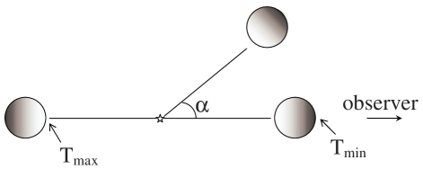
Figure 2.— Clouds at a fixed distance from the AGN at various position angles $\alpha$ with respect to the observer direction. The dust temperature varies on the surface of an optically thick cloud from $T_{\rm max}$ on the illuminated face to $T_{\rm min}$ on the dark side. Therefore the emission is anisotropic and $\alpha$ determines the visible fraction of the illuminated surface area.

3. SOURCE FUNCTION

The formalism just described is general. Its application to a specific radiative process requires modeling of the source function for a single cloud. Here we apply this formalism to dusty torus clouds heated by the central AGN radiation. We divide the clouds into two classes. For large optical depths, clouds directly facing the AGN will have a higher temperature on the illuminated face than on other surface areas (Fig. 2). Their emission is therefore strongly anisotropic, and the corresponding source function $S^{\rm d}_{\rm c,\lambda}$ depends on both distance $r$ from the AGN and the angle $\alpha$ between the directions of the cloud and observer. Clouds whose view of the AGN is blocked by another cloud will be heated only indirectly by all other clouds. Heating of these clouds by diffuse radiation is, in general, much more even, and the $\alpha$-dependence is expected to be much weaker for their source function $S^{\rm i}_{\rm c,\lambda}$ than for $S^{\rm d}_{\rm c,\lambda}$. At location $(r,\beta)$, the mean number of clouds to the AGN is $\hbox{$\cal N$}(r,\beta)=\int_{0}^{r}\!\hbox{$N_{\rm C}$}(r,\beta)\,dr$ and the probability for unhindered view of the AGN is $p(r,\beta)=e^{-{\cal N}(r,\beta)}$. The general expression for the cloud overall source function at that location is thus

$$\hbox{$S_{\rm c,\lambda}$}(r,\alpha,\beta)=p(r,\beta)\hbox{$S^{\rm d}_{\rm c,\lambda}$}(r,\alpha)+\left[1-p(r,\beta)\right]\hbox{$S^{\rm i}_{\rm c,\lambda}$}(r,\alpha,\beta)$$ (10)

We now describe our detailed calculations of the source functions of the two classes of clouds.

3.1. Directly illuminated clouds

Clouds come in all shapes and forms. But whatever its shape, when the size of a cloud directly illuminated by the AGN is much smaller than $r$, it is indistinguishable from a flat patch with the same overall optical depth. Indeed, all calculations of line emission from AGN always model the line emitting clouds as slabs illuminated by the central engine along the normal to their surface. However, a fundamental difference between a flat slab and an actual cloud of the same optical thickness is that the former presents to an observer either its bright or dark faces while the latter generally presents a combination of both. To account for this effect we construct “synthetic clouds” by averaging the emission from an illuminated slab over all possible slab orientations (figure 3). This procedure utilizes an exact solution of radiative transfer for externally illuminated slabs, and we proceed now to discuss the properties of an irradiated dusty slab; the synthetic clouds are constructed from the slab solutions in §3.1.4.

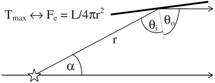
Figure 3.— A synthetic cloud at distance $r$ from the AGN and position angle $\alpha$ from the observer direction is constructed by averaging the emission from a slab with the same optical depth over all slab orientations (see eq. 16). The local illuminating flux, $F_{\rm e}$, and maximal temperature on the cloud surface, $T_{\rm max}$, are uniquely related to each other (see §3.1.2).

3.1.1 Slab radiative transfer

Thanks to the planar symmetry, the slab radiative transfer equation can be formulated completely in optical depth space; neither the density profile nor the slab geometrical thickness are relevant. In the case of dusty slabs this invariance extends to the temperature equation because the only attenuation of the heating radiation comes from radiative interactions. Therefore the slab radiative transfer problem is fully specified by the optical depth $\hbox{$\tau_{\rm\lambda}$}=q_{\lambda}\hbox{$\tau_{\rm V}$}$, where $\tau_{\rm V}$ is the dust optical depth across the slab at visual wavelengths and $q_{\lambda}$ is the relative efficiency factor at wavelength $\lambda$. The radiative transfer equation along a ray at angle $\arccos\mu$ to the slab normal is

$$\mu{d\hbox{$I_{\lambda}$}\over d\hbox{$\tau_{\rm\lambda}$}}=S_{\lambda}(\hbox{$\tau_{\rm\lambda}$})-\hbox{$I_{\lambda}$}(\hbox{$\tau_{\rm\lambda}$})$$ (11)

where $\tau_{\rm\lambda}$ is measured in the normal direction from the illuminated face and $S_{\lambda}$ is the source function. For dust albedo $\varpi_{\lambda}$ and isotropic scattering, $S_{\lambda}=(1-\hbox{$\varpi_{\lambda}$})\hbox{$B_{\lambda}$}(T)+\hbox{$\varpi_{\lambda}$}\hbox{$J_{\lambda}$}$ where $J_{\lambda}$ is the angle averaged intensity and $T$ the dust temperature, obtained at each point in the slab from the coupled equation of radiative equilibrium.

We solve the slab radiative transfer problem with the 1D code DUSTY (Ivezić, Nenkova, & Elitzur, 1999). The code takes advantage of the scaling properties of the radiative transfer problem for dust absorption, emission and scattering (Ivezić & Elitzur, 1997, IE97 hereafter). The solution determines both the radiation field and the dust temperature profile in the slab. The dust grains are spherical with size distribution from Mathis, Rumpl, & Nordsieck (1977). The composition has a standard Galactic mix of 53% silicates and 47% graphite. The optical constants for graphite are from Draine (2003), for silicate from the Ossenkopf, Henning, & Mathis (1992) “cold dust”, which produces better agreement with observations of the 10 and 18 $\mu$m silicate features (Sirocky et al., 2008). From the optical constants DUSTY calculates the absorption and scattering cross-sections using the Mie theory and replaces the grain mixture with a single-type composite grain whose radiative constants are constructed from the mix average. This method reproduces adequately full calculations of grain mixtures, especially when optical depths are large (e.g., Efstathiou & Rowan-Robinson, 1994; Wolf, 2003). The handling of the dust optical properties is exact in this approach, the only approximation is in replacing the temperatures of the different grain components at each point in the slab with a single average. Wolf (2003) finds that the temperatures of different grains are within $\hbox{$\sim$}\pm 10\%$ of that obtained in the mean grain approximation, and that these deviations disappear altogether when $\tau>10$. Henceforth, the term “dust temperature” implies this mean temperature of the mixture.

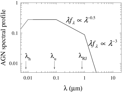
Figure 4.— The spectral shape of the AGN illuminating radiation for the standard set of parameters (see eq. 13).

The slab is illuminated by the AGN flux $F_{\rm e,\lambda}$ at an angle $\theta_{\rm i}$ from the normal. For isotropic AGN emission with luminosity $L$, the bolometric flux at the slab position is

$$\hbox{$F_{\rm e}$}={L\over 4\pi r^{2}}$$ (12)

The illuminating flux is characterized by $F_{\rm e}$ and by the AGN normalized SED $\hbox{$f_{\rm e\lambda}$}=F_{\rm e,\lambda}/\hbox{$F_{\rm e}$}$. Following Rowan-Robinson (1995), we employ the piecewise power-law distribution

$$\lambda\hbox{$f_{\rm e\lambda}$}\propto\cases{\lambda^{1.2}&\hskip 14.45377pt$\lambda\leq\hbox{$\lambda_{\rm h}$}$\cr\rm const&\hskip 14.45377pt$\hbox{$\lambda_{\rm h}$}\leq\lambda\leq\hbox{$\lambda_{\rm u}$}$\cr\lambda^{-p}&\hskip 14.45377pt$\hbox{$\lambda_{\rm u}$}\leq\lambda\leq\hbox{$\lambda_{\rm RJ}$}$\cr\lambda^{-3}&\hskip 14.45377pt$\hbox{$\lambda_{\rm RJ}$}\leq\lambda$\cr}$$ (13)

with the following set of parameters: $\lambda_{\rm h}$ = 0.01$\mu$m, $\lambda_{\rm u}$ = 0.1$\mu$m, $\lambda_{\rm RJ}$ = 1$\mu$m and $p$ = 0.5 (see fig. 4). The effects of varying the parameters from this standard set are discussed below in §3.1.5.

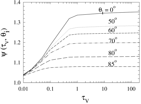
Figure 5.— The effects of optical thickness $\tau_{\rm V}$ (normal to the slab sides) and illumination angle $\theta_{\rm i}$ on the temperature of the slab illuminated surface. Shown is the variation of the function $\psi$ (see eq. 14) with $\tau_{\rm V}$ at various $\theta_{\rm i}$, as marked. The dust in all figures has standard Galactic composition, the temperature is the mixture average. The flatness of $\psi$ for $\hbox{$\tau_{\rm V}$}\gtrsim 1$ implies that the dust temperature is the same on the illuminated face of all optically thick slabs.

3.1.2 Dust temperature

When $\hbox{$\tau_{\rm V}$}\ll 1$ the diffuse radiation inside the slab is negligible. The dust temperature is the same everywhere in the slab and depends only on $F_{\rm e}$; it does not depend on either $\tau_{\rm V}$ or the illumination angle $\theta_{\rm i}$ (so long as the slab remains optically thin along the slanted direction). The same holds for any externally heated cloud as long as it is optically thin and its size is much smaller that the distance to the source, and the slab geometry faithfully mimics this aspect. By contrast, when the radiation source is embedded inside a smooth density distribution (e.g., a spherical shell), the dust temperature does vary even in the optically thin case because of the spatial dilution of radiation with distance from the source.

When $\hbox{$\tau_{\rm V}$}>1$ the slab diffuse radiation contributes significantly to dust heating. If $q_{\rm a\lambda}$ is the efficiency factor for absorption, let $\hbox{$q_{\rm ae}$}=\int\!\hbox{$q_{\rm a\lambda}$}\hbox{$f_{\rm e\lambda}$}d\lambda$ and $q_{\rm aP}$ the corresponding average with the Planck spectral shape. From radiative equilibrium, the dust temperature at the slab illuminated boundary obeys (IE97)

$$\sigma T^{4}\hbox{$q_{\rm aP}$}(T)=\frac{1}{4}\hbox{$F_{\rm e}$}\hbox{$q_{\rm ae}$}\psi(\hbox{$\tau_{\rm V}$},\hbox{$\theta_{\rm i}$})$$ (14)

The function $\psi$ introduced here accounts for the contribution of the diffuse radiation to the energy density, and can be obtained only from a detailed solution of the radiative transfer problem; it is normalized according to $\psi(0,\hbox{$\theta_{\rm i}$})=1$ to recover the temperature of optically thin dust (IE97). Irrespective of the actual value of the dust temperature on the illuminated face, the function $\psi$ fully describes the effects of illumination angle and slab overall optical depth on that temperature. Figure 5 shows the variation of $\psi$ with both $\tau_{\rm V}$ and $\theta_{\rm i}$. The dependence on either variable is weak. Even for normal illumination, where it is the largest, $\psi$ does not exceed 1.35, reaching its maximum at $\hbox{$\tau_{\rm V}$}\gtrsim 1$; i.e., the contribution of the diffuse component to the surface heating is no more than 35% of the direct heating by the external source. This behavior is markedly different from the spherical case where $\psi$ increases monotonically with $\tau_{\rm V}$ without bound (IE97). The reason is the fundamental difference in the relation between radiative flux and energy density in the two geometries. In a spherical shell, the energy density can increase indefinitely in the inner cavity because there is no energy transport there (from symmetry, the diffuse flux vanishes in the cavity). As the optical depth increases, the radiation trapped in the cavity dominates the dust heating on the shell inner boundary, leading to an unbounded increase of $\psi$ with $\tau_{\rm V}$ (the same surface temperature requires a smaller $F_{\rm e}$). In contrast, a slab cannot store energy anywhere. When a slab optical thickness increases, any increase in diffuse energy density is accompanied by a commensurate flux increase, producing the saturation effect evident in the figure. As a result, the temperature on the illuminated face is the same, independent of optical depth when $\hbox{$\tau_{\rm V}$}\gtrsim 1$.

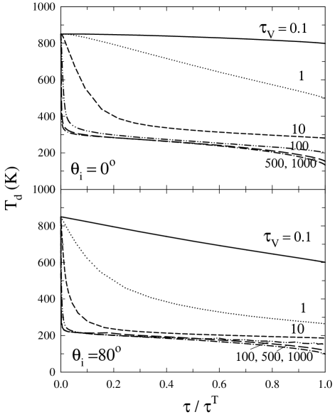
Figure 6.— Temperature variation inside slabs of various $\tau_{\rm V}$, as marked, for two illumination angles. The variable $\tau/\tau^{\rm T}$ is thickness into the slab from the illuminated face, where the temperature is 850 K for all the displayed slabs.

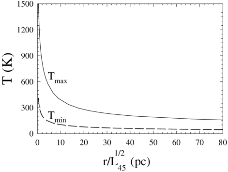
Figure 7.— An optically thick dusty slab at distance $r$ from an AGN with luminosity $L_{45}=L$/($10^{45}$ erg s^-1) is irradiated normal to the surface. The dust temperature is $T_{\rm max}$ on the slab illuminated face, $T_{\rm min}$ on the dark side. The curve for $T_{\rm max}$ is applicable whenever $\hbox{$\tau_{\rm V}$}>1$, the one for $T_{\rm min}$ when $\hbox{$\tau_{\rm V}$}>10$.

Figure 6 displays the temperature variation inside representative slabs of varying optical thickness heated to a surface temperature of 850 K. After a sharp drop near the illuminated face, the temperature is nearly constant throughout the rest of the slab for optical depths exceeding $\tau_{\rm V}$ $\sim$ 10. There is little difference between the profiles at large overall optical depths—all slabs with $\tau_{\rm V}$ $\geq$ 100 produce nearly indistinguishable profiles. Increasing $\theta_{\rm i}$ has a similar effect to increasing $\tau_{\rm V}$ because of the slanted illumination. The temperature decline near the illuminated surface reflects the exponential attenuation of the external heating radiation. Once this radiation is extinguished, the dust temperature in the rest of the slab is maintained by the diffuse radiation. And since the bolometric flux is constant and must be radiated from the slab dark side, this temperature is uniquely determined by the external flux and the grain optical properties. It is independent of the overall optical depth once that optical depth exceeds unity for all wavelengths around the Planck peak. This behavior is in stark contrast with all centrally heated dust distributions where the flux radiated from the outer boundary decreases as the surface area increases with overall size, leading to ever declining dust temperatures.

As is evident from figure 5, $\psi(\hbox{$\tau_{\rm V}$},\hbox{$\theta_{\rm i}$})$ is nearly constant as a function of $\tau_{\rm V}$ for $\hbox{$\tau_{\rm V}$}\geq 1$; deviations are within the 5% accuracy of our numerical results. Therefore, at a given distance $r$ from the AGN and a given inclination $\theta_{\rm i}$, all optically thick slabs are heated to the same surface temperature. And as is evident from figure 6, they also have essentially the same dust temperature on their dark face when $\hbox{$\tau_{\rm V}$}>10$. Figure 7 displays the variation of these two surface temperatures with distance from the AGN for optically thick slabs with normal illumination. The displayed relations can be described with simple analytic approximations. The temperature $T_{\rm max}$ on the illuminated face reaches 1500 K at distance $R_{\rm d}\simeq 0.4\,L_{45}^{1/2}$ pc, where $L_{45}=L$/($10^{45}$ erg s^-1). Introduce $\rho=r/\hbox{$R_{\rm d}$}$, then

$$T_{\rm max} \simeq \cases{1500\cdot(1/\rho)^{0.39}\ \hbox{K}&$\rho\leq 9$\cr\cr\phantom{1}640\cdot(9/\rho)^{0.45}\ \hbox{K}&$\rho>9$\cr}$$

$$T_{\rm min} \simeq \phantom{1}400\cdot(1/\rho)^{0.42}\ \hbox{K}$$ (15)

These temperatures bracket the range of dust temperatures on the surface of a cloud at distance $\rho$ from the AGN (see figure 2). Because the dust temperature is determined by radiative equilibrium, the large disparity between different surface areas cannot be equalized by cloud rotation. The dust is primarily heated by absorption of short wavelength radiation in electronic transitions, with typical time scales of $10^{-6}$ sec, and cools via vibrational transitions within seconds. Therefore dust radiative equilibrium is established instantaneously when compared with any dynamical time scale. It is also important to note that the gas has no effect on the dust temperature as long as the density is $\lesssim$ $10^{12}$ cm^-3.

All the clouds illustrated in figure 2 are at the same distance from the AGN, yet their radiation toward the observer involves a mix of a wide range of surface temperatures. This result has profound implications for the torus emission. The 10 $\mu$m dust emission in NGC1068 has been recently resolved in VLTI interferometry by Jaffe et al. (2004), who analyzed their observations with a model containing a compact ($r\lesssim$ 0.5 pc) hot ($>$ 800 K) core and cooler (320 K) dust extending to $r\simeq$ 1.7 pc. Poncelet et al. (2006) reanalyzed the same data with slightly different assumptions and reached similar conclusions — the coolest component in their model has an average temperature of 226 K and extends to $r$ = 2.7 pc. As noted by the latter authors, the close proximity of regions with dust temperature of $>$ 800 K on one hand and $\sim$200–300 K on the other is a most puzzling, fundamental problem. Clumpiness provides a natural solution, thanks to the spatial collocation of widely different dust temperatures. With a bolometric luminosity of $\sim$ 2$\times$$10^{45}$ erg s^-1 for NGC1068 (Mason et al., 2006), the dust temperature in an optically thick cloud at $r$ = 2 pc is 960 K on the bright side but only 247 K on the dark side, declining further to 209 K at 3 pc. Indeed, the temperatures deduced in the model synthesis of the VLTI data fall inside the range covered by the cloud surface temperatures at the derived distances. Schartmann et al. (2005) have recently modeled the NGC1068 torus with multi-grain dust in a smooth density distribution and found that, although the different dust components span at the same location a range of temperatures, this range is smaller than required. They conclude that even with this refinement their model cannot explain the VLTI interferometric observations and that the clumpy structure of the dust configuration must be included in realistic modeling. The same effect is found in the Circinus AGN, where Tristram et al. (2007) conclude similarly that the temperature distribution inferred from their VLTI observations provides strong evidence for a clumpy or filamentary dust structure.

At a given distance $r$, the highest surface temperature is obtained for slab orientation normal to the radius vector. This maximal temperature has a one-to-one correspondence with $F_{\rm e}$. Thanks to this correspondence, $T_{\rm max}$ can be used instead of $F_{\rm e}$ to characterize the boundary condition of the solution.

3.1.3 Emerging intensity from a slab

The spectral shape of the radiation emerging from the slab depends on $\tau_{\rm V}$, $T_{\rm max}$, $\theta_{\rm i}$ and the angle $\theta_{\rm o}$ between the observer direction and the slab normal (see figure 3). Figures 8–10 display the dependence of the slab SED on these four parameters. Each figure displays separately the SEDs for the illuminated and dark sides of the slab, which are fundamentally different from each other. Every SED is scaled with $F_{\rm e}$, the AGN bolometric flux at the slab location (see eq. 12).

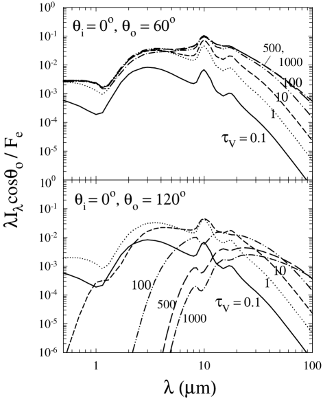
Figure 8.— Optical depth dependence of SED of slabs illuminated by normal radiation to $T_{\rm max}$ = 850 K. In the top and bottom panels the observer direction is 60$\arcdeg$ from slab normal on the illuminated and dark sides, respectively.

Figure 8 displays the $\tau_{\rm V}$ dependence of the SED for representative parameters. On the illuminated side the SED is dominated by scattering and hot emission from the surface layer. The silicate 10$\mu$m feature appears always in emission, although its contrast decreases with $\tau_{\rm V}$. On the dark side, the feature displays the behavior familiar from spherical models (e.g., IE97): emission at small $\tau_{\rm V}$, switching to absorption at large $\tau_{\rm V}$ when the hot radiation from the illuminated region propagates through optically thick cool layers. However, the absorption feature is never as deep as in the spherical case , reflecting the flat temperature profile (fig. 6).

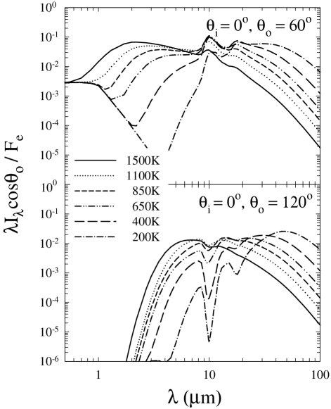
Figure 9.— The SED of slabs with $\tau_{\rm V}$ = 100 normally illuminated to surface temperature $T_{\rm max}$, as marked. All other parameters are the same as in Fig. 8.

Figure 9 shows the variation of the SED with the temperature of the illuminated surface. The change in temperature affects the dust emission, shifting it to longer wavelengths as $T$ decreases. This modifies the 10$\mu$m silicate feature. When the emission peak moves past 10$\mu$m, the silicate feature starts disappearing from the SED. Short wavelengths ($\lambda\lesssim 1\hbox{$\mu$m}$) are dominated by the scattered component. They are visible only on the bright side and are unaffected by this change.

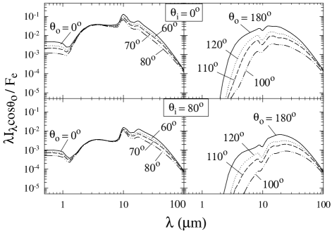
Figure 10.— Dependence of slab SED on illumination and observation angles $\theta_{\rm i}$ and $\theta_{\rm o}$. The observer is on the illuminated side in the left panels, on the dark side in the right panels. All slabs have $\tau_{\rm V}$ = 100, the external flux $F_{\rm e}$ corresponds to $T_{\rm max}$ = 850 K (the surface temperature that a normally illuminated slab would have at that location).

Figure 10 shows the effects of the illumination and viewing angles. Moving the observer’s direction away from the slab normal has a similar effect to increasing the slab optical depth. Varying the illumination angle affects the attenuation of the external heating radiation.

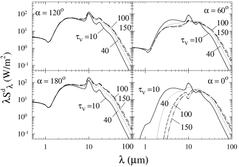
Figure 11.— Dependence of the source function of directly illuminated clouds on optical depth. The clouds are located at $r$-equivalent temperature $T_{\rm max}$ = 850 K and position angles as marked; $\alpha=0\arcdeg$ is directly in front of the AGN, $\alpha=180\arcdeg$ directly behind (see fig. 2).

3.1.4 Cloud source function $S^{\rm d}_{\rm c,\lambda}$

A slab-like patch observed at angle $\theta_{\rm o}$ from a large distance appears as a point whose intensity (flux per solid angle) is $\hbox{$I_{\lambda}$}(\hbox{$\theta_{\rm o}$})\cos\hbox{$\theta_{\rm o}$}$. At a distance $r$ from the AGN, corresponding to temperature $T_{\rm max}$, and position angle $\alpha$ we construct the source function for a “synthetic cloud” with optical depth $\tau_{\rm V}$ from

$$\hbox{$S^{\rm d}_{\rm c,\lambda}$}(\hbox{$T_{\rm max}$},\hbox{$\tau_{\rm V}$},\alpha)=\langle I(\hbox{$T_{\rm max}$},\hbox{$\tau_{\rm V}$},\hbox{$\theta_{\rm i}$},\hbox{$\theta_{\rm o}$})\cos\hbox{$\theta_{\rm o}$}\rangle$$ (16)

Here $\hbox{$I_{\lambda}$}(\hbox{$T_{\rm max}$},\hbox{$\tau_{\rm V}$},\hbox{$\theta_{\rm i}$},\hbox{$\theta_{\rm o}$})$ is the intensity of a slab with the listed parameters and the brackets denote averaging over all possible slab orientations (Fig. 3). The fraction of slabs with observable bright side is the same as the visible fraction of the illuminated area on the surface of a spherical-like cloud.

Figure 11 displays the dependence of the source function $S^{\rm d}_{\rm c,\lambda}$ on optical depth for clouds located at the same distance at a number of representative position angles around the AGN. At $\alpha=0\arcdeg$, only the dark side of the cloud is visible (see fig. 2). Increasing $\alpha$ exposes to the observer a larger fraction of the illuminated area until it is fully visible at $\alpha=180\arcdeg$. This explains the emergence of short wavelengths and the switch from absorption to emission of the 10 $\mu$m silicate feature as $\alpha$ increases. The same behavior is evident also in figure 12, which provides a more detailed coverage of the $\alpha$-dependence of $S^{\rm d}_{\rm c,\lambda}$ as well as additional temperatures.

At all position angles, increasing the optical depth of a single cloud beyond $\hbox{$\tau_{\rm V}$}\sim 100$ has only a minimal effect on the spectral shape. And except for the short wavelengths at $\alpha=0$, the SED similarity extends down almost to clouds with $\tau_{\rm V}$ = 10. This behavior reflects the saturation of the slab temperature profile (see fig. 6) and is a realistic depiction of the situation inside an actual cloud heated from outside by a distant source. An important consequence of the flatness of the temperature profile through most of the cloud is that the silicate absorption feature never becomes deep — a uniform temperature source cannot produce an absorption feature at all. This is fundamentally different from continuous dust distributions surrounding the heating source, where the temperature keeps decreasing with radial distance and the absorption feature keeps getting deeper as the overall optical depth increases until finally the entire wavelength region is suppressed by self absorption. In an externally heated cloud, on the other hand, the depth of the absorption feature is set by the contrast between temperatures on the two faces. When both $T_{\rm max}$ and $T_{\rm min}$ are higher than $\sim$ 300 K (the Planck-equivalent of 10$\mu$m, roughly) the entire slab contributes to 10$\mu$m emission; when both are lower, no region emits appreciably at this wavelength. The absorption feature is deepest when the hot face is warmer than $\sim$ 300 K and the cool side is cooler, maximizing the contrast between the emitting and absorbing layers. The solutions displayed in figure 12 for $T_{\rm max}$ = 400K and 200K show the deepest absorption features produced by directly illuminated clouds for any combination of the parameters.

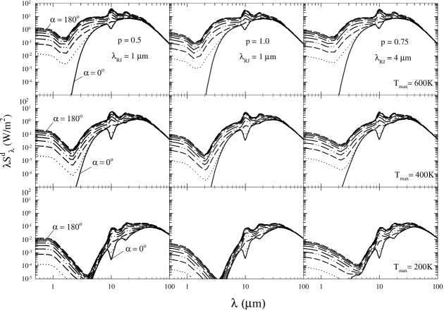
Figure 12.— Dependence of the source function for directly illuminated clouds with $\tau_{\rm V}$ = 100 on position angle $\alpha$, varied at $20\arcdeg$ intervals. Each row of panels corresponds to $r$-equivalent temperature $T_{\rm max}$ as marked. Each column corresponds to a different set of $p$ and $\lambda_{\rm RJ}$ (see eq. 13) for the illuminating spectral shape, with the central one corresponding to the standard parameters .

3.1.5 The input spectral shape

All previous descriptions of the spectral shape of the AGN input continuum are summarized by the piecewise power law in eq. 13 (see Rowan-Robinson, 1995, and references therein). The continuum shape shortward of 0.1$\mu$m (1000Å) is uncertain; the slope of the spectral falloff between optical and X-rays has been determined for many sources but the location $\lambda_{\rm h}$ of the turndown from flat $\lambda\hbox{$f_{\rm e\lambda}$}$ toward high frequencies remains unknown. Fortunately, this spectral region has no effect on the shape of the dust SED. It affects only the normalization of the relation between luminosity and dust temperature (eq. 3.1.2), and we find this to be only $\sim$ 1% effect when $\lambda_{\rm h}$ increases from our standard 0.01$\mu$m all the way to 0.03$\mu$m.

The impact of the optical—near-IR region is much more significant. Since dust cannot be hotter than its sublimation temperature ($\sim$ 1500 K), it emits predominantly at $\lambda\gtrsim$ 2–3$\mu$m. Shorter wavelengths involve the Wien tail of emission by the hottest dust and scattering of the AGN radiation, and thus reflect directly the input spectrum. We characterize the AGN emission in this region by the spectral index $p$ and the wavelength $\lambda_{\rm RJ}$, which marks the onset of the Rayleigh-Jeans tail $\hbox{$f_{\rm e\lambda}$}\propto\lambda^{-4}$. This wavelength corresponds roughly to the lowest temperature on the accretion disk of the central engine. The spectral index $p$ has been determined for 6868 quasars studied in the Sloan Digital Sky Survey (Ivezić et al., 2002). Its distribution covers the range $-1\leq p\leq 1.5$ and has a flat peak at $0.5\leq p\leq 0.8$. Direct observational determination of $\lambda_{\rm RJ}$ requires near-IR spectral studies of type 1 AGN with angular resolution better than 0$\farcs$01 for a source distance of 10 Mpc. Such observations are yet to be performed. Promising indirect methods for separating the near-IR emission into its torus and disk components include measurements of continuum polarization (Kishimoto et al., 2005) and multiple regression analysis of time variability (Tomita et al., 2006).

Figure 12 shows SEDs for clouds illuminated by radiation with $p$ = 0.5 and $p$ = 1, two cases that bracket the peak of the observed $p$-distribution. The input spectrum makes no difference at wavelengths dominated by dust emission, $\lambda\gtrsim$ 2$\mu$m. Shorter wavelengths are dominated by the AGN scattered radiation, and the displayed results reflect the difference in input radiation in this spectral region. Although not large, these differences are important because IR spectral indices that include at least one wavelength shorter than 2$\mu$m are a common tool of spectral analysis (e.g., Alonso-Herrero et al., 2003). The figure also shows an intermediate slope, $p$ = 0.75, with $\lambda_{\rm RJ}$ increased from 1$\mu$m to 4$\mu$m. As is evident from the figure, such an increase will also produce an observable effect on IR spectral indices.

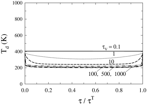
Figure 13.— Temperature variation inside slabs of various $\tau_{\rm V}$, as marked, heated indirectly by diffuse radiation at distance from the AGN with equivalent temperature $T_{\rm max}$ = 850 K (cf fig. 6). The variable $\tau/\tau^{\rm T}$ is thickness into the slab from one face.

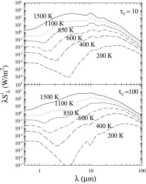
Figure 14.— Source functions of clouds heated indirectly by the diffuse radiation for two optical depths and a set of distances, labelled by the equivalent temperature $T_{\rm max}$.

3.2. Clouds Heated Indirectly

Clouds whose line-of-sight to the AGN is blocked by another cloud will be heated only indirectly by the diffuse radiation from all other clouds. Just as in the standard, smooth density case, the self-consistent solution for the coupled problems of diffuse radiation field and source function can be readily obtained by $\Lambda$-iterations. In the first step, calculate the source functions for all directly heated clouds, and from the emission of these clouds devise a first approximation for the diffuse radiation field. Next, place clouds in this radiation field and calculate their emission to derive a first approximation for the source functions of indirectly illuminated clouds and, from eq. 10, the composite source function at every location. In successive iterations, add to the AGN direct field the cloud radiation calculated from eq. 5, and repeat the process until convergence. The solution must be tested for flux conservation, which takes the same form in both the smooth and clumpy cases: $\int\!d\lambda\int\!F_{\rm r,\lambda}(r,\Omega)d\Omega/4\pi=\hbox{$F_{\rm e}$}$, where the angular integration is over a spherical Gaussian surface of radius $r$ and $F_{\rm r,\lambda}$ is the radial component of the radiative flux vector, comprised of the AGN transmitted radiation and the diffuse dust emission. In clumpy distributions, the contribution of the transmitted flux to this integral becomes $p_{\rm AGN}$$F_{\rm e}$, where $p_{\rm AGN}$ is from eq. 8, and the radial component of the diffuse flux at any position is $F_{\rm r,\lambda}^{\rm C}=\int\hbox{$I^{\rm C}_{\lambda}$}\cos\theta d\Omega$, where $I^{\rm C}_{\lambda}$ is the intensity from eq. 5 and $\theta$ is angle to the radius vector. Thus the flux conservation relation becomes

$$\hbox{$p_{\rm AGN}$}\hbox{$F_{\rm e}$}+\int_{0}^{1}\!\!d\sin\beta\int\!d\lambda\,F_{\rm r,\lambda}^{\rm C}(r,\beta)=\hbox{$F_{\rm e}$}\,.$$ (17)

With trivial modifications, this is also the result for the smooth-density case: in the transmitted term ($p_{\rm AGN}$$F_{\rm e}$) the clumpy effective optical depth $t_{\lambda}$ is replaced by actual optical depth $\tau_{\lambda}$ in the escape factor $P_{\lambda,\rm esc}$, and in the diffuse term $I^{\rm C}_{\lambda}$ stands for the smooth-density emission intensity.

Dust is heated predominantly at short wavelengths and is reprocessing radiation toward longer wavelengths. As a result, at every location the clouds heated directly by the AGN will be the warmest and provide much stronger heating than the shadowed, much cooler clouds. The significance of feedback from the clouds that are heated indirectly can be gauged from $\hbox{$S^{\rm i}_{\rm c,\lambda}$}/\hbox{$S^{\rm d}_{\rm c,\lambda}$}$, the ratio of their source function to the driving term $S^{\rm d}_{\rm c,\lambda}$; when this ratio is small, rapid convergence can be expected. In our calculations we performed only the first two steps of the $\Lambda$-iteration process and employed an isotropic radiation field as an approximation for the heating of shadowed clouds. The approximate heating field was derived from an average over $\alpha$ of the emission of directly heated clouds at the given location; this is the radiation field that would exist inside a spherical shell of directly illuminated clouds at the given location. In reality, an indirectly heated cloud is probably exposed to the bright sides of somewhat fewer clouds, because they are on the far side from the AGN, so our approximation is an upper limit for the strength of the diffuse field. In this isotropic field we placed dusty slabs and solved the radiative transfer problem with DUSTY. Figure 13 shows the temperature profile inside such slabs at the location where $T_{\rm max}$ = 850 K. As expected, slabs heated by the diffuse radiation are much cooler than their directly illuminated counterparts, shown in fig. 6. As before, from the radiative transfer solution we obtained $S^{\rm i}_{\rm c,\lambda}$ using the averaging procedure in eq. 16. Since now the slab is illuminated isotropically on both faces, the dependence on $\theta_{\rm i}$ disappears and $S^{\rm i}_{\rm c,\lambda}$ is isotropic. Figure 14 shows results for $S^{\rm i}_{\rm c,\lambda}$ at two representative optical depths and a range of radial distances, characterized by $T_{\rm max}$. Figure 15 shows the corresponding ratio $S^{\rm i}_{\rm c,\lambda}$/$S^{\rm d}_{\rm c,\lambda}$ for $\tau_{\rm V}$ = 100. This ratio is always below $\sim$10% around the wavelengths corresponding to peak emission at each distance; for example, clouds with $T_{\rm max}$ = 200 are the main contributors to the emission around $\sim$15$\mu$m, and as is evident from the figure, $S^{\rm i}_{\rm c,\lambda}$ is less than 10% of $S^{\rm d}_{\rm c,\lambda}$ for this temperature in that spectral range. Significantly, $S^{\rm i}_{\rm c,\lambda}$/$S^{\rm d}_{\rm c,\lambda}$ is small even though our approximation overestimates the diffuse radiation strength as it involves an isotropic distribution of directly heated clouds around every AGN-obscured cloud. As expected, clouds heated indirectly are much weaker emitters, indicating rapid convergence of the iteration procedure.

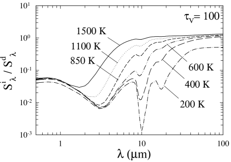
Figure 15.— Ratio of the source functions for directly- and indirectly-heated clouds with $\tau_{\rm V}$ = 100 at the indicated distance-equivalent temperatures. $S^{\rm d}_{\lambda}$ is taken at $\alpha=90\arcdeg$.

In contrast with figs. 11 and 12, figure 14 shows only a trace of the 10 $\mu$m feature. This disparity reflects the fundamental differences, evident in figures 6 and 13, between the internal temperature structures of directly- and indirectly-illuminated clouds. A cloud placed in a black-body radiation field will thermalize with its temperature $T$ and emit according to $I_{\lambda}=B_{\lambda}(T)(1-e^{-\tau_{\lambda}})$. Therefore, when ${\tau_{10\hbox{$\mu$m}}\ll 1}$, $I_{\lambda}\simeq B_{\lambda}\tau_{\lambda}$ and the emergent spectrum has the same shape as the dust cross section, producing an emission feature. When $\tau_{10\hbox{$\mu$m}}$ increases and approaches unity, self-absorption sets in and the feature strength decreases. As $\tau_{10\hbox{$\mu$m}}$ increases further and exceeds unity, $I_{\lambda}$ becomes equal to $B_{\lambda}$: at constant temperature, self-absorption and emission exactly balance each other, producing the thermodynamic limit of the Planck function. For all $\tau_{10\hbox{$\mu$m}}>1$, a single-temperature cloud will never produce a feature, either in emission or absorption. Since our diffuse radiation field differs from a pure black-body, the temperature inside indirectly heated clouds is not constant, but its variation is still relatively modest, as is evident from fig. 13. While the dust temperature in a directly illuminated slabs varies by more than factor 4, it varies by less than factor 2 inside slabs heated from both sides by the isotropic diffuse radiation field. Furthermore, even this small variation is mostly limited to narrow regions near the heated surfaces. This explains why fig. 14 shows only a weak emission feature at $\tau_{\rm V}$ = 10 (which corresponds to $\tau_{10\hbox{$\mu$m}}\simeq 0.7$) and practically no feature in most of the $\tau_{\rm V}$ = 100 clouds.

4. DISCUSSION

The formalism presented here is general and can be applied to any clumpy distribution. In this study we employed it to construct the source functions of dusty clouds. As a small object, a cloud is primarily characterized by its overall optical depth $\tau_{\rm V}$. Two additional properties could potentially affect the cloud emission. One is surface smoothness. A rough, fractal-like surface can be expected to reduce the efficiency of scattering by absorbing some scattered photons and transferring them to the thermal pool. The other is shape. This factor could be studies by averaging ellipsoidal clouds over all orientations. The shape parameter would then correspond to the ellipsoid axial ratio as the cloud varied from a spherical shape to extreme elongation; the clouds constructed here can be considered representative of extremely elongated shapes. The isotropy of the external radiation field of indirectly heated clouds enabled us to explore in this case the two extremes of cloud geometrical shape: since the radiative transfer problem for a spherical cloud retains the spherical symmetry in an isotropic external field, it too can be solved by DUSTY. The source function is then found from $\hbox{$S^{\rm i}_{\rm c,\lambda}$}=F_{\lambda}/\Omega$, where $F_{\lambda}$ and $\Omega$ are, respectively, the flux and solid angle of the sphere at a large distance. We calculated $S^{\rm i}_{\rm c,\lambda}$ for spherical clouds imbedded in the same radiation field used in the calculations described in §3.2. The solution for a sphere with uniform density depends only on the overall optical depth $\tau_{\rm V}$, allowing direct comparison with the clouds constructed by averaging slabs of the same $\tau_{\rm V}$. We found no significant differences between the two extreme cases. We are currently studying also the direct illumination of spherical clouds, and will report our full findings in a separate publication (Kimball, Ivezić & Elitzur, in preparation).

Both shape and surface properties appear to be of secondary importance. The modeling of the source function presented here in which the clouds are characterized purely by $\tau_{\rm V}$ does seem to capture the essence of emission from a single dusty cloud, although definitive conclusions will have to await detailed comparisons with the calculations for externally illuminated spheres.

4.1. Dust temperature in clumpy media

Dust temperature distributions are profoundly different in clumpy and smooth media. In smooth density distributions, dust temperature and distance from the AGN are uniquely related to each other—given the distance, the dust temperature is known, and vice versa. In contrast, as shown in §3.1.2, in a clumpy medium

• different dust temperatures coexist at the same distance from the AGN

• the same dust temperature occurs at different distances — the dark side of a cloud close to the AGN can be as warm as the bright side of a farther cloud

Schartmann et al. (2005) find that different components of the multi-grain mix employed in their torus modeling can have different temperatures at the same location, therefore the concept of “dust temperature” is ill defined at the microscopic level in such regions. Still, the fundamental differences between the temperature structures of smooth and clumpy media apply to the individual components of the grain mix and to the mixture average, as well as to the common, proper dust temperature when all the components equilibrate to the same one. These differences have profound implications for the torus emission, explaining the low dust temperatures found so close to the nuclei of NGC1068 (Jaffe et al., 2004; Poncelet et al., 2006) and Circinus (Tristram et al., 2007). We discuss these implications further in part II.

4.2. X-rays vs IR

IR flux measurements collect the emission from the entire torus area on the plane of the sky. This flux is determined by the average number of clouds along all radial rays through the torus. In contrast, X-ray attenuation is controlled by the clouds along just one particular ray, the line of sight to the AGN. Since X-rays are absorbed by dust-free as well as dusty material, X-ray absorbing clouds will generally outnumber the torus clouds in any given direction. In fact, X-ray absorption in AGN could be dominated by the dust-free clouds (see paper II). But even for the dusty portion of the column, the number of X-ray absorbing clouds can differ substantially from the torus average. As an example, the appendix table 1 presents a tabulation of the Poisson distribution for $\cal N$ = 5, which is representative of AGN tori as shown in part II. More than 80% of the paths will have a number of clouds different from 5 in this case, and the probability to encounter just 1 cloud or as many as 9 is a full 20% of the probability to encounter the average 5. Two type 2 sources with similar cloud properties and the same average $\cal N$ will have an identical IR appearance, yet the X-ray absorbing columns in each torus could still differ by an order of magnitude. This can be expected to introduce a large scatter in X-ray observations.

Each spectral regime responds to large variations in cloud optical depth in an entirely different way. The IR emission depends on $\tau_{\rm V}$ through the probability for photon escape and the cloud source function (see eq. 5). Both factors saturate when $\tau_{\rm V}$ exceeds $\sim$100. From eq. 4, $\hbox{$P_{\rm esc}$}=e^{-\cal N}$ when $\tau_{\lambda}\gg 1$. Since this condition is met at all relevant wavelengths when $\hbox{$\tau_{\rm V}$}\gtrsim 50$, $P_{\rm esc}$ becomes independent of $\tau_{\rm V}$. Similarly for $S_{\rm c,\lambda}$: Because each cloud is heated from outside, only its surface is heated significantly when $\tau_{\rm V}$ is large. Increasing $\tau_{\rm V}$ further only adds cool material, thus $S_{\rm c,\lambda}$ saturates for all relevant $\lambda$ (similar to standard black-body emission). Indeed, figure 11 displays model results that cover three orders of magnitude of clump optical depth, yet the SEDs show only moderate variation, saturating altogether when $\hbox{$\tau_{\rm V}$}\gtrsim 100$. Even at $\hbox{$\tau_{\rm V}$}<100$, significant spectral variety is mostly limited to $\lambda\lesssim 10$ $\mu$m for clouds along the line of sight to the AGN. In contrast, the $\tau_{\rm V}$-dependence of X-ray absorption is markedly different. Individual torus clouds are optically thin to X-rays, because the optical depth for Thomson scattering is only $\sim$2$\times$$10^{-3}$$\tau_{\rm V}$, therefore the overall optical depth for X-ray absorption is $\cal N$$\tau_{\rm V}$ (see §2.1). It increases linearly with $\tau_{\rm V}$, in contrast with the saturated response in the IR regime.

The great disparity between the two spectral regions is expected to further increase the scatter in torus X-ray properties among AGN with similar IR emission. It also may help explain why the SEDs show only moderate variations in the infrared that are not well correlated with the X-ray absorbing columns (e.g., Silva et al., 2004).

4.3. The 10$\mu$m feature

In contrast with ultra-luminous infrared galaxies (ULIRGs), AGN observations do not provide any example of deep 10$\mu$m silicate absorption feature (Hao et al., 2007). This behavior conflicts with the results of smooth-density models (e.g., Pier & Krolik, 1992) but is a natural consequence of clumpiness: as is evident from figures 11 and 12, single clumps never produce extremely deep features. This behavior reflects the flat slab temperature profile (see fig. 6) and is a realistic depiction of the situation inside an actual cloud heated from outside by a distant source. As noted by Levenson et al. (2007), the different behavior of the 10$\mu$m absorption in ULIRGs and AGN indicates that the dust distribution is smooth in the former and clumpy in the latter (see also Spoon et al., 2007).

Clumpiness suffices by itself to explain the modest depth of the 10 $\mu$m absorption feature in AGN. The complete behavior of the feature, including the transition from emission to absorption, involves an intricate interplay between the relative contributions of clouds at different locations and their mutual shadowing. This behavior displays a complex pattern that depends on the actual geometry of the cloud distribution. A detailed, quantitative analysis of the 10$\mu$m feature in clumpy tori is performed in part II.

4.4. Conclusions

Clumpy media differ from continuous ones in a number of fundamental ways. The low dust temperatures found close to the nucleus of NGC1068 contradict basic physical principles in smooth density distributions but arise naturally in clumpy ones. Two additional puzzling features of IR emission from AGN are simply hallmarks of clumpy dust distributions, independent of the distribution geometry: Even if the cloud configurations were spherical or irregular rather than toroidal, (1) the SED still would show only a moderate range incommensurate with the variation of X-ray attenuation, and (2) the 10$\mu$m absorption feature would never be deep. Understanding the full range of 10$\mu$m features observed in AGN spectra requires considerations of the actual geometry of the cloud distribution, though. This problem is addressed in part II together with other implications of clumpy tori to AGN observations.

Appendix A Poisson Statistics

Table 1

$k$	$P_{k}$	$P_{k}/P_{\cal N}$	$\sum\limits_{i\leq k}P_{i}$
0	0.0067	0.04	–
1	0.0337	0.19	0.04
2	0.0842	0.48	0.12
3	0.1404	0.80	0.27
4	0.1755	1.00	0.44
5	0.1755	1.00	0.62
6	0.1462	0.83	0.76
7	0.1044	0.60	0.87
8	0.0653	0.37	0.93
9	0.0363	0.21	0.97
10	0.0181	0.10	0.99
11	0.0082	0.05	0.99
12	0.0034	0.02	1.00

The elementary problem most relevant for the statistics of clouds along a ray is the distribution of points placed randomly on a circular board. Denote by $n$ the total number of points and by $p\ (\ll 1)$ the probability that a point lands on a given radial ray. Then the probability for $k$ points to land on that ray is

$$P_{k}={n!\over k!(n-k)!}\,p^{k}(1-p)^{n-k}$$ (A1)

If $\cal N$ is the average number of points landing on a ray than $p~{}=~{}\hbox{$\cal N$}/n$, therefore

$$P_{k}={\hbox{$\cal N$}^{k}\over k!}\left(1-{\hbox{$\cal N$}\over n}\right)^{n}\times\left[\left(1-{1\over n}\right)\!\!\left(1-{2\over n}\right)\ldots\left(1-{k+1\over n}\right)\left(1-{\hbox{$\cal N$}\over n}\right)^{-k}\right]$$ (A2)

In the limit $n\to\infty$ with $\cal N$ and $k$ fixed, every term in the square brackets approaches unity while $(1-\hbox{$\cal N$}/n)^{n}\to e^{-\cal N}$, yielding the Poisson distribution

$$P_{k}\simeq{\hbox{$\cal N$}^{k}\over k!}e^{-\cal N}.$$ (A3)

Equation 4 for the photon escape probability follows immediately. The probability to encounter $k$ clouds along the path is $P_{k}$. If the optical depth of each cloud is $\tau$ then the probability to escape from all of these encounterers is $e^{-k\tau}$. Therefore

$$\hbox{$P_{\rm esc}$}=\sum_{k}P_{k}e^{-k\tau}=e^{-\cal N}\sum_{k}{(\hbox{$\cal N$}e^{-\tau})^{k}\over k!}$$ (A4)

yielding the Natta & Panagia result (eq. 4).

It is important to note that the only requirement for eq. A3 is that the total number of points obey $n\gg k,\hbox{$\cal N$}$; the mean number $\cal N$ of points on a ray can be small (even less than unity). While the statistics of points along a ray always follows the Poisson distribution, there is no similar universal limit for the statistics of the average $\cal N$, and it remains arbitrary. As an example, consider a large number of identical boards with the same number of points $n$ spread on each one of them, so that the average $\cal N$ is the same for every board. In this case $\cal N$ will have a $\delta$-function distribution while the number of points on any given ray in each board will obey the Poisson distribution around that common average.

Finally, the Poisson distribution allows significant deviations from the average. From the accompanying tabulation for $\cal N$ = 5, the probability to hit just one cloud or as many as nine clouds is 20% of the probability to hit the average five clouds. This implies a substantial probability that the number of clouds along any particular line of sight, such as the one to the AGN, will deviate significantly from the torus average $\cal N$.

References

- Alonso-Herrero et al. (2003) Alonso-Herrero, A., Quillen, A. C., Rieke, G. H., Ivanov, V. D., & Efstathiou, A. 2003, AJ, 126, 81
- Antonucci (1993) Antonucci, R. 1993, ARA&A, 31, 473
- Antonucci (2002) Antonucci, R. 2002, in Astrophysical Spectropolarimetry, ed. J. Trujillo-Bueno, F. Moreno-Insertis, & F. Sánchez, 151–175
- Conway et al. (2005) Conway, J., Elitzur, M., & Parra, R. 2005, Ap&SS, 295, 319
- Draine (2003) Draine, B. T. 2003, ApJ, 598, 1017
- Efstathiou & Rowan-Robinson (1994) Efstathiou, A., & Rowan-Robinson, M. 1994, MNRAS, 266, 212
- Elitzur (2006) Elitzur, M. 2006, New Astronomy Review, 50, 728
- Elitzur (2007) Elitzur, M. 2007, in ASP Conf. Ser. 373: The Central Engine of Active Galactic Nuclei, ed. L. C. Ho & J.-M. Wang, 415–424
- Elitzur et al. (2004) Elitzur, M., Nenkova, M., & Ivezić, Ž. 2004, in ASP Conf. Ser. 320: The Neutral ISM in Starburst Galaxies, ed. S. Aalto, S. Huttemeister, & A. Pedlar, 242–252
- Hao et al. (2007) Hao, L., Weedman, D. W., Spoon, H. W. W., Marshall, J. A., Levenson, N. A., Elitzur, M., & Houck, J. R. 2007, ApJ, 655, L77
- Hönig et al. (2006) Hönig, S. F., Beckert, T., Ohnaka, K., & Weigelt, G. 2006, A&A, 452, 459
- Ivezić & Elitzur (1997) Ivezić, Ž., & Elitzur, M. 1997, MNRAS, 287, 799
- Ivezić et al. (2002) Ivezić, Ž. et al. 2002, AJ, 124, 2364
- Ivezić et al. (1999) Ivezić, Ž., Nenkova, M., & Elitzur, M. 1999, User manual for DUSTY, University of Kentucky Internal Report, accessible at http://www.pa.uky.edu/~moshe/dusty/
- Jaffe et al. (2004) Jaffe, W. et al. 2004, Nature, 429, 47
- Kaspi & Netzer (1999) Kaspi, S., & Netzer, H. 1999, ApJ, 524, 71
- Kishimoto et al. (2005) Kishimoto, M., Antonucci, R., & Blaes, O. 2005, MNRAS, 364, 640
- Krolik & Begelman (1988) Krolik, J. H., & Begelman, M. C. 1988, ApJ, 329, 702
- Levenson et al. (2007) Levenson, N. A., Sirocky, M. M., Hao, L., Spoon, H. W. W., Marshall, J. A., Elitzur, M., & Houck, J. R. 2007, ApJ, 654, L45
- Maiolino et al. (2007) Maiolino, R., Shemmer, O., Imanishi, M., Netzer, H., Oliva, E., Lutz, D., & Sturm, E. 2007, A&A, 468, 979
- Mason et al. (2006) Mason, R. E., Geballe, T. R., Packham, C., Levenson, N. A., Elitzur, M., Fisher, R. S., & Perlman, E. 2006, ApJ, 640, 612
- Mathis et al. (1977) Mathis, J. S., Rumpl, W., & Nordsieck, K. H. 1977, ApJ, 217, 425
- Natta & Panagia (1984) Natta, A., & Panagia, N. 1984, ApJ, 287, 228
- Nenkova et al. (2002) Nenkova, M., Ivezić, Ž., & Elitzur, M. 2002, ApJ, 570, L9
- Nenkova et al. (2008) Nenkova, M., Sirocky, M. M., Nikutta, R., Ivezić, Ž., & Elitzur, M. 2008, ApJ, submitted
- Netzer (1990) Netzer, H. 1990, in Active Galactic Nuclei, ed. T. J. L. Courvoisier & M. Mayor, 57
- Ossenkopf et al. (1992) Ossenkopf, V., Henning, T., & Mathis, J. S. 1992, A&A, 261, 567
- Pier & Krolik (1992) Pier, E. A., & Krolik, J. H. 1992, ApJ, 401, 99
- Poncelet et al. (2006) Poncelet, A., Perrin, G., & Sol, H. 2006, A&A, 450, 483
- Rowan-Robinson (1995) Rowan-Robinson, M. 1995, MNRAS, 272, 737
- Schartmann et al. (2005) Schartmann, M., Meisenheimer, K., Camenzind, M., Wolf, S., & Henning, T. 2005, A&A, 437, 861
- Silva et al. (2004) Silva, L., Maiolino, R., & Granato, G. L. 2004, MNRAS, 355, 973
- Sirocky et al. (2008) Sirocky, M. M., Levenson, N. A., Elitzur, M., Spoon, H. W. W., & Armus, L. 2008, ApJ, 678, 729
- Spoon et al. (2007) Spoon, H. W. W., Marshall, J. A., Houck, J. R., Elitzur, M., Hao, L., Armus, L., Brandl, B. R., & Charmandaris, V. 2007, ApJ, 654, L49
- Tomita et al. (2006) Tomita, H. et al. 2006, ApJ, 652, L13
- Tristram et al. (2007) Tristram, K. R. W. et al. 2007, A&A, 474, 837
- Urry & Padovani (1995) Urry, C. M., & Padovani, P. 1995, PASP, 107, 803
- Wolf (2003) Wolf, S. 2003, ApJ, 582, 859