A Study of Quasar Proximity in O vi absorbers at $z$=2–3

Abstract

With the goal of investigating the nature of O vi absorbers at high redshifts, we study the effects of proximity to the background quasar. In a sample of sixteen quasars at $z_{\rm qso}$ between 2.14 and 2.87 observed at high signal-to-noise and 6.6 km s^-1 resolution with VLT/UVES, we detect 35 O vi absorption-line systems (comprising over 100 individual O vi components) lying within 8 000 km s^-1 of $z_{\rm qso}$. We present component fits to the O vi absorption and the accompanying H i, C iv, and N v. The systems can be categorized into 9 strong and 26 weak O vi absorbers. The strong (intrinsic) absorbers are defined by the presence of either broad, fully saturated O vi absorption or partial coverage of the continuum source, and in practice all have log $N$(O vi)$\ga$15.0; these systems are interpreted as representing either QSO-driven outflows or gas close the central engine of the AGN. The weak (also known as narrow) systems show no partial coverage or saturation, and are characterized by log $N$(O vi)$<$14.5 and a median total velocity width of only 42 km s^-1. The incidence d$N$/d$z$ of weak O vi systems within 2 000 km s^-1 of the quasar down to a limiting equivalent width of 8 mÅ is 42$\pm$12. Between 2 000 and 8 000 km s^-1, d$N$/d$z$ falls to 14$\pm$4, equal to the incidence of intervening O vi absorbers measured in the same spectra. Whereas the accompanying H i and C iv column densities are significantly lower (by a mean of $\sim$1 dex) in the weak O vi absorbers within 2 000 km s^-1 of $z_{\rm qso}$ than in those at larger velocities, the O vi column densities display no dependence on proximity. Furthermore, significant offsets between the H i and O vi centroids in $\approx$50 per cent of the weak absorbers imply that (at least in these cases) the H i and O vi lines are not formed in the same phase of gas, preventing us from making reliable metallicity determinations, and ruling out single-phase photoionization-model solutions. In summary, we find no firm evidence that quasar radiation influences the weak O vi absorbers, suggesting they are collisionally ionized rather than photoionized, possibly in the multi-phase halos of foreground galaxies. Non-equilibrium collisional ionization models are needed to explain the low temperatures in the absorbing gas, which are implied by narrow line widths ($b\!<\!14$ km s^-1) in over half of the observed O vi components.

1 Introduction

Quasars are ideal backlights for absorption-line spectroscopy, thanks to their high luminosities and flat continua. Yet in addition to allowing us to detect foreground absorbers, quasars also create and influence them, through the effects of outflows and ionizing radiation. The enhanced level of ionizing radiation in the vicinity of quasars gives rise to the line-of-sight proximity effect, the observed decrease in the number density of Ly$\alpha$ forest lines (equivalent to a decrease in the mean optical depth, and an increase in the level of hydrogen ionization) at velocities approaching the quasar (Carswell et al., 1982; Murdoch et al., 1986; Tytler, 1987; Bajtlik, Duncan, & Ostriker, 1988; Lu, Wolfe, & Turnshek, 1991; Bechtold, 1994; Rauch, 1998; Scott et al., 2000; Guimarães et al., 2007; Faucher-Giguère et al., 2008).

To obtain an unbiased view of absorbing structures in the high-$z$ Universe, one needs to remove the effects of proximity from samples of metal-line systems. The broad absorption line (BAL) systems, easy to identify in QSO spectra because of their optically thick absorption extending over thousands of km s^-1, are clearly connected to the quasar. BALs trace high-velocity QSO outflows at speeds of up to 0.1$c$ (e.g. Turnshek, 1984, 1988), and are seen in 10–15% of quasar spectra at $z\!>\!1.5$ (Weymann et al., 1991; Trump et al., 2006). A separate category of mini-BAL systems, with fully saturated absorption profiles and total velocity width $<$ 2 000 km s^-1, has also been identified (Turnshek, 1988; Churchill et al., 1999; Yuan et al., 2002; Misawa et al., 2007b). As with BALs, mini-BALs are interpreted as tracing outflows ejected by QSOs. A more difficult task is to decide whether narrow absorbers in quasar spectra are either created by or ionized by the QSO. The traditional way to do this employs the displacement velocity from the quasar, $\delta v\!\equiv\!v_{\rm qso}\!-\!v_{\rm abs}$. So-called ‘associated’ or ‘$z_{\rm abs}\!\approx\!z_{\rm qso}$’ or ‘proximate’ absorbers, typically defined as narrow absorbers at $\delta v\!<\!5\,000$ km s^-1 (Weymann et al., 1979; Foltz et al., 1986; Anderson et al., 1987; Hamann & Ferland, 1999) are often removed from intervening samples because of the possibility they may be intrinsic. Arguments in favour of an intrinsic nature for many proximate absorbers include time-variability of absorption, partial coverage of the continuum source, detection of excited ionic states implying high gas densities, profiles that are smoother than intervening absorbers, and super-solar metallicities (Wampler, Bergeron, & Petitjean, 1993; Møller, Jakobsen, & Perryman, 1994; Petitjean, Rauch, & Carswell, 1994; Savaglio, D’Odorico, & Møller, 1994; Tripp et al., 1996; Barlow & Sargent, 1997; Hamann, 1997; Hamann et al., 1997a, c, 2001; Hamann, Netzer, & Shields, 2000; Petitjean & Srianand, 1999; Srianand & Petitjean, 2000; Ganguly et al., 1999, 2001, 2006; Narayanan et al., 2004).

Using a velocity cutoff to differentiate intervening and intrinsic absorbers has two main problems: quasar-ejected intrinsic systems can appear at higher $\delta v$ (Hamann, Barlow, & Junkkarinen, 1997b; Richards et al., 1999; Richards, 2001; Misawa et al., 2007a; Nestor, Hamann, & Rodríguez Hidalgo, 2008), and intervening systems can appear at lower $\delta v$ (Møller, Warren, & Fynbo, 1998; Sembach et al., 2004). So are many genuine intervening systems lost when they are excluded from absorber samples just because of their proximity to the quasar? In this paper we investigate the transition between proximate and intervening absorbers. We focus on O vi absorbers, which trace either warm-hot ($T\!\ga\!10^{5}$ K) collisionally-ionized plasma, or photoionized gas subject to a hard ionizing spectrum extending to energies above 113.9 eV (the ionization potential to create O⁺⁵). O vi absorbers are of interest for many reasons, including the significant role they play in the baryon and metal budgets, the window they provide on intergalactic metal enrichment, and their ability to trace energetic galaxy/IGM interactions such as accretion and galactic winds. After the first detection of O vi absorbers at $z$=2–3 by Lu & Savage (1993), much work has been done in the era of 10m-class telescopes to characterize their properties (Schaye et al., 2000; Carswell, Schaye, & Kim, 2002; Bergeron et al., 2002; Simcoe, Sargent, & Rauch, 2002, 2004, 2006; Bergeron & Herbert-Fort, 2005; Lopez et al., 2007; Aguirre et al., 2008; Gonçalves, Steidel, & Pettini, 2008).

Here we ask a simple question: is there a proximity effect in O vi? In other words, can we see the signature of quasar photoionization, in terms of correlations between the ionization properties of absorbers and their proximity to the quasar? To address this issue, we form a sample of proximate O vi absorption systems at $z$=2–3 using a homogeneous set of high-resolution VLT/UVES quasar spectra, and we then compare their properties to a sample of intervening (i.e., non-proximate) O vi absorbers observed in the same set of spectra; the intervening sample has been published by Bergeron & Herbert-Fort (2005, hereafter BH05), but it has since been enlarged from ten to twelve sight lines. We also briefly compare our results on O vi absorbers at $z$=2–3 to those obtained in the low-redshift Universe with space-based ultraviolet spectrographs. This paper is thus a study of both the proximity effect and the nature of O vi absorbers in general, and is structured as follows. In §2 we describe the data acquisition and reduction, and our absorber identification and measurement processes. In §3 we discuss the observational properties of proximate O vi absorbers. In §4 we discuss the implications of our results, and we then present a summary in §5. Throughout this paper we adopt a WMAP 3-year cosmology with $\Omega_{\rm M}$=0.27, $\Omega_{\Lambda}$=0.73, and $h_{\rm 70}$=1 (Spergel et al., 2007).

2 Data Acquisition and Handling

2.1 Observations

The ESO-VLT Large Programme The Cosmic Evolution of the Intergalactic Medium (IGM) has built a homogeneous sample of high resolution, high signal-to-noise quasar spectra for use in studying the high-redshift IGM. Twenty bright quasars (most with $V\!<\!17$) in the redshift range 2.1–3.8 (median $z_{\rm qso}$=2.44) were selected for observation, deliberately avoiding sight lines that contain high-column density damped Ly$\alpha$ absorbers. The observations were carried out with the Ultraviolet and Visual Echelle Spectrograph (UVES; Dekker et al., 2000) on VLT UT2 at Paranal, Chile, using a total of thirty nights of service-mode telescope time between June 2001 and September 2002. The observations were taken in good seeing conditions ($<$0.8″) and at airmass$<$1.4, with both blue and red dichroics (Dic1 346+580, Dic1 390+564, and Dic2 437+860 settings), giving spectra complete from 3 000 to 9 000 Å. The data reduction was conducted using the MIDAS pipeline described in Ballester et al. (2000), and then continua were fitted using a third-degree spline function interpolated between regions free from absorption. Full details of the reduction process are given in Chand et al. (2004) and Aracil et al. (2004). The 2$\times$2 binning mode was used, giving a rebinned pixel size of 2.0–2.4 km s^-1. The spectral resolution of the data, $R\approx 45\,000$, corresponds to a velocity resolution of $\approx$6.6 km s^-1 (FWHM). Typical signal-to-noise ratios per pixel in the spectra are $\approx$35 at 3 500 Å and $\approx$60 at 6 000 Å. Among the twenty quasars, sixteen are at $z\!<\!3$. These form the basic sample for this paper. The four cases at $z\!>\!3$ were excluded, because the density of the Ly$\alpha$ forest at these redshifts renders futile searches for O vi.

The emission-line redshifts of ten of the sixteen quasars in our sample have been carefully determined by Rollinde et al. (2005, and references therein), and we adopt their values. For the remaining six quasars we take $z_{\rm qso}$ from Scannapieco et al. (2006). Each of these quasar redshifts is based on a combination of the observed H$\alpha$, Mg ii, C iv, and Si iv emission-line redshifts, allowing for systematic shifts in the displacement velocities of the various lines (e.g. Tytler & Fan, 1992). The uncertainty on each $z_{\rm qso}$ is of the order 500 km s^-1 (Rollinde et al., 2005).

2.2 Identification of O vi systems

We searched systematically through the sixteen quasar spectra in our sample for O vi absorbers within 8 000 km s^-1 of the quasar redshift. This velocity range corresponds to redshifts between $z_{\rm min}$=$z_{\rm qso}$–[(1+$z_{\rm qso}$) 8 000 km s^-1/c] and $z_{\rm qso}$. Our choice of velocities up to 8 000 km s^-1 from the quasar was made in order to investigate whether a transition occurs at 5 000 km s^-1, the conventional cutoff between proximate and intervening systems. In practise, we also searched for (and found) O vi absorbers at up to 2 500 km s^-1 beyond the quasar redshift, indicating the presence of high-velocity inflows toward the quasar.

32 O vi absorbers were identified by their presence in both lines of the O vi $\lambda\lambda$1031.926, 1037.617 doublet in the correct ratio through the line profile, i.e. $\tau_{a}(v,\lambda 1031)/\tau_{a}(v,\lambda 1037)=2$, where the apparent optical depth $\tau_{a}(v)={\rm ln}\,[F_{c}(v)/F(v)]$, and where $F(v)$ and $F_{c}(v)$ are the observed flux level and estimated continuum flux level, respectively, as a function of velocity. In addition, three O vi absorbers were identified in one line of the O vi doublet only, with partial blending in the other O vi line, but with corresponding absorption seen in C iv and H i at exactly the same redshift. Together the sample consists of the 35 O vi systems listed in Table 1. We define the system redshift $z_{\rm abs}$ by the position of the strongest O vi component in the system, i.e. the wavelength of maximum optical depth. In each system, we looked for accompanying absorption in H i (Ly$\alpha$, Ly$\beta$, and Ly$\gamma$), C iii $\lambda 977$, C iv $\lambda\lambda 1548,1550$, and N v $\lambda\lambda 1238,1242$ at the same redshift $z_{\rm abs}$.

We denote the velocity displacement of each absorber from the quasar as $\delta v\equiv c|z_{\rm qso}\!-\!z_{\rm abs}|/(1\!+\!z_{\rm abs})$. A negative value corresponds to an absorber moving toward the quasar. The O vi systems almost always contain multiple components clustered together. We thus define $\delta v$ both for each absorber and for each individual O vi component. The uncertainties on all velocity displacements are dominated by the $\approx$500 km s^-1 uncertainty of the quasar emission redshifts.

2.3 Classification of O vi systems

After identifying 35 proximate O vi systems, we found that they could be classified into:

(a) Seven strong O vi systems, which are defined by showing both fully saturated O vi lines extending over tens to hundreds of km s^-1, and strong (often saturated) N v and C iv absorption. In practice we find that these seven systems all show log $N$(O vi)$>$15.0 and are at $\delta v\!<\!3\,000$ km s^-1, with four of the seven at $\delta v<0$ ($z_{\rm abs}$$>$$z_{\rm qso}$), i.e. the strong systems are strongly clustered around $z_{\rm qso}$. The strong systems are interpreted as being intrinsic to the quasar. Three of the strong systems are classified as mini-BALs, but no full (classical) BAL systems are present in our sample. Partial coverage of the continuum source is present in many of the strong systems, as evidenced by the failure to find a successful Voigt profile fit to the O vi profiles, even though the velocity structure is common among the two members of the doublet. This confirms an intrinsic origin, because partial coverage of the continuum source only occurs when the absorbing gas is physically close to the AGN. The strong systems contain multiple components, with a mean of 5.9 components per system.

(b) 26 weak O vi systems, also known as narrow systems, which are unsaturated and show no evidence for partial coverage, i.e. we were able to conduct successful Voigt profile fits to the two lines of the O vi doublet. The weak systems all have 12.80$<$log $N$(O vi)$<$14.50, clearly separated from the strong systems, but coincident with the range of O vi column densities observed in intervening systems (BH05). Their total line widths are narrow, with a median and standard deviation of $\Delta v_{90}$=42$\pm$33 km s^-1, where $\Delta v_{90}$ is the line width encompassing the central 90% of the integrated optical depth. The weak O vi systems are accompanied by C iv absorption in 24/26 cases, and in 9/26 cases by N v. An mean of 1.9 components per system is required to fit these weak absorbers.

There were two intermediate cases that presented difficulties in their classification: the systems at $z$=2.6998 and 2.7134 toward HE 0151-4326. Neither of these systems shows a saturated O vi profile, and their O vi column densities lie in-between the values shown by the strong ($>$15.0) and weak ($<$14.5 populations). However, differences between the profiles of the two doublet lines of O vi, and between the two lines of N v, in similar velocity ranges are strongly suggestive of partial coverage. This implies they should be classified as intrinsic. For this reason we place these systems in the strong category, and our final sample consists of 9 strong systems and 26 weak systems.

In addition to the different O vi (and N v and C iv) column densities, there are several lines of evidence that support the notion that the strong and weak samples trace physically different populations. The strong population have velocities (relative to $z_{\rm qso}$) that distribute differently, with 4/9 at $z_{\rm abs}$$>$$z_{\rm qso}$, whereas 22/26 weak absorbers are at $z_{\rm abs}$$<$$z_{\rm qso}$. The strong population are show markedly different H i/O vi ratios than the weak population (see §3.5). Finally absorbers in the strong population frequently show evidence for partial coverage of the continuum source. Whereas the strong absorbers are clearly associated with the quasar (e.g. Turnshek, 1984; Weymann et al., 1991; Hamann & Ferland, 1999), either tracing QSO outflows or inflows near the central engine of the AGN, the origin of the weak O vi absorbers is less clear. They are often called ‘associated’ because of their proximity in velocity to the quasar, but there is not necessarily any physical connection. In the rest of this paper we investigate the properties of this weak, proximate sample.

2.4 Component fitting

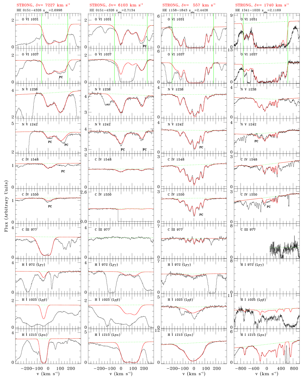
Figure 1: Absorption-line spectra of all proximate O vi systems in the UVES Large Programme. Strong absorbers are shown first, followed by the weak absorbers. Our Voigt profile fits are shown in red. In many of the C iv and N v panels, the data are shown over a limited range in the y-axis, for clarity. Green vertical lines indicate the velocity range of the AOD integration. The label ‘PC’ indicates regions where partial coverage of the continuum source affects the line profiles. At the top of each column we annotate our classification and the proximity of the absorber to the quasar.

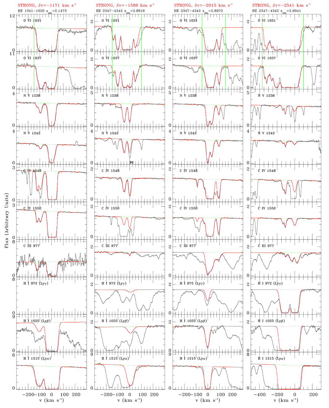
Figure 1: (cont.)

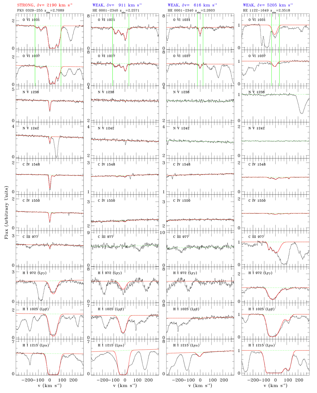
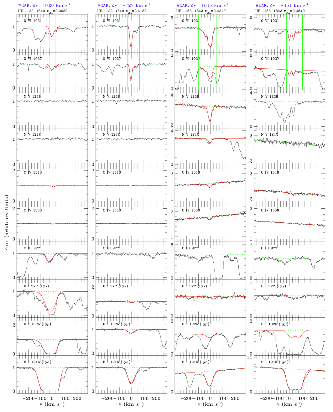
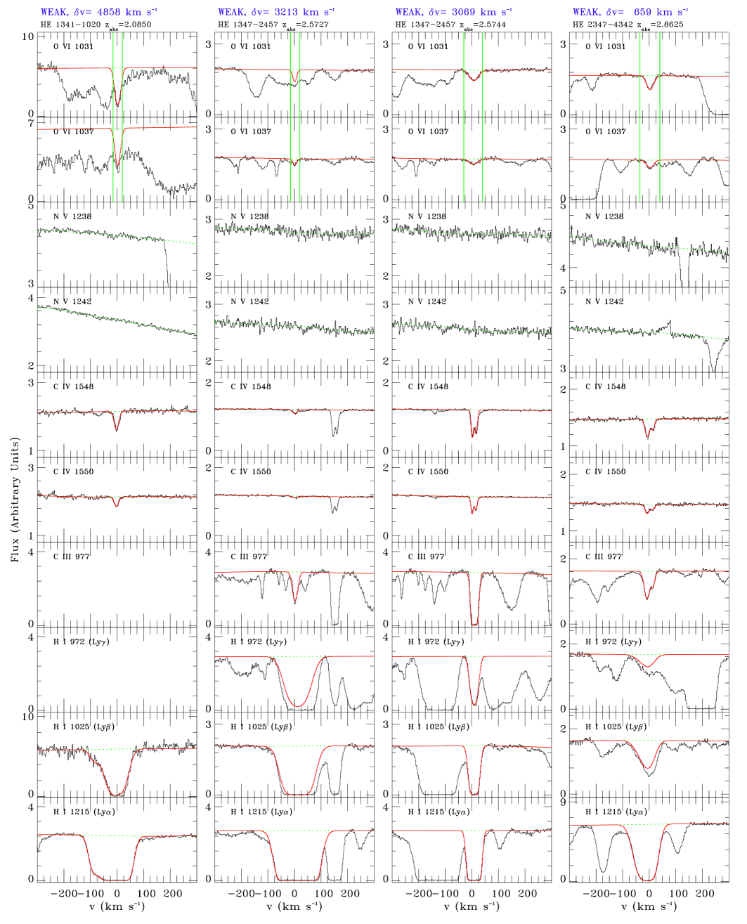
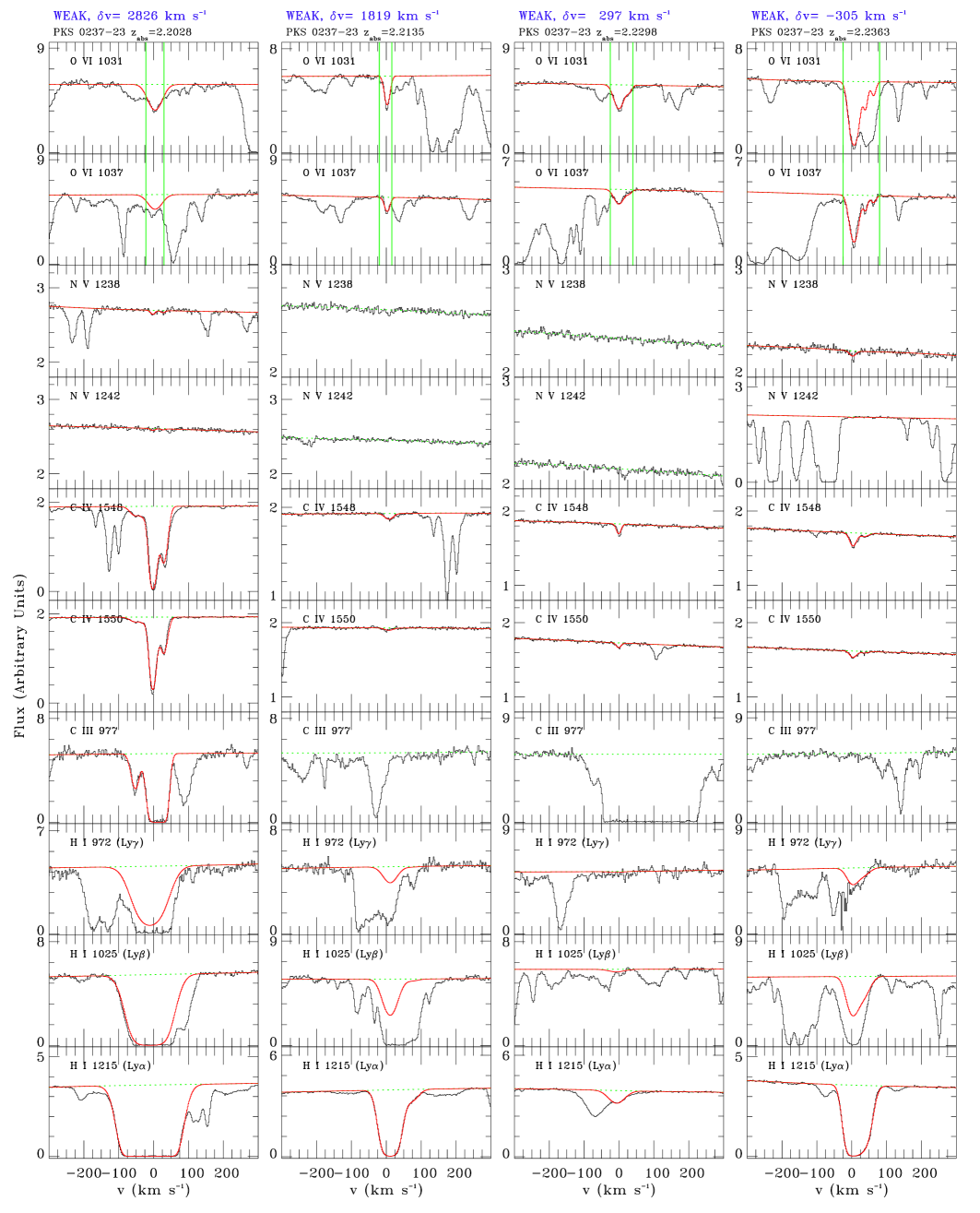
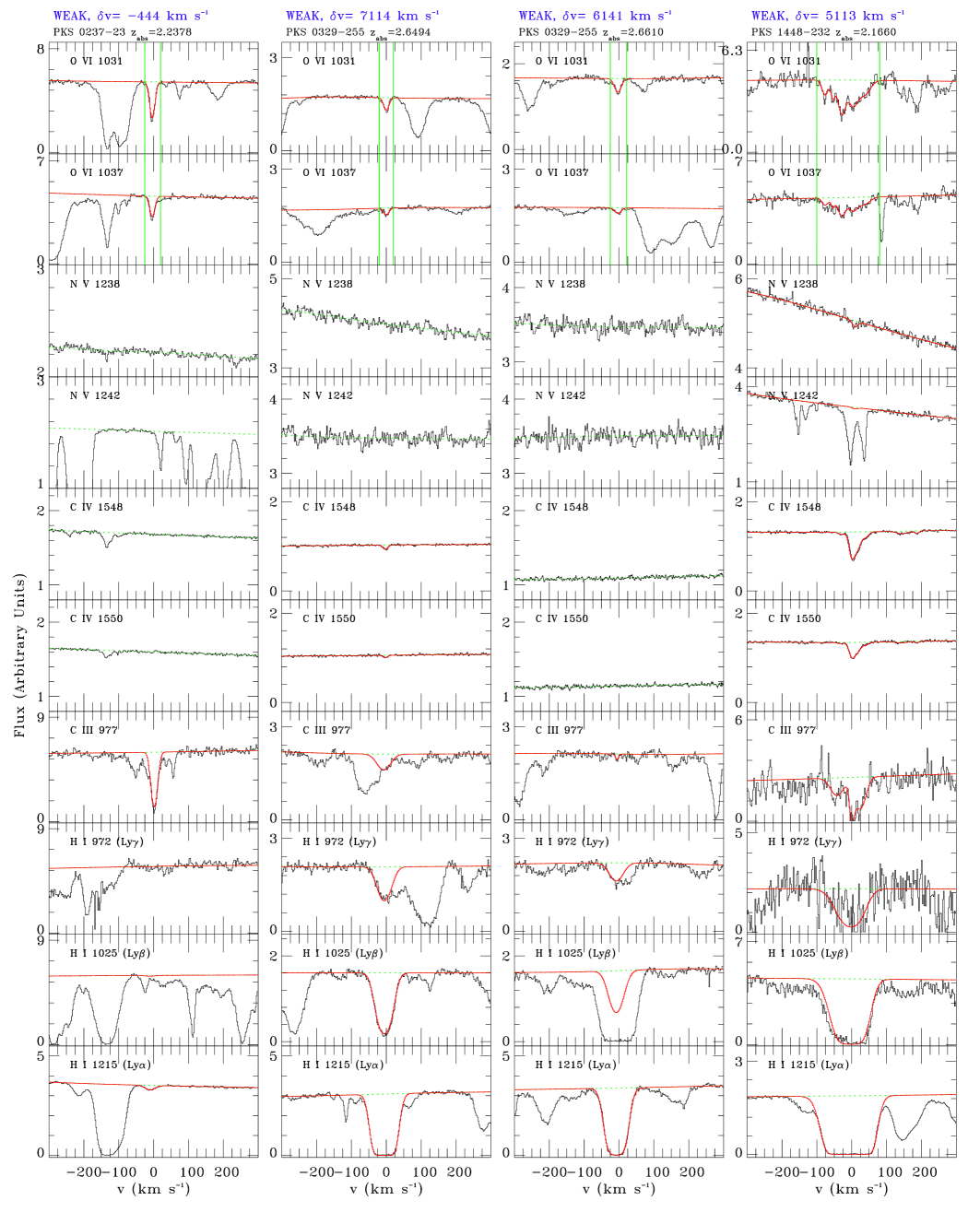
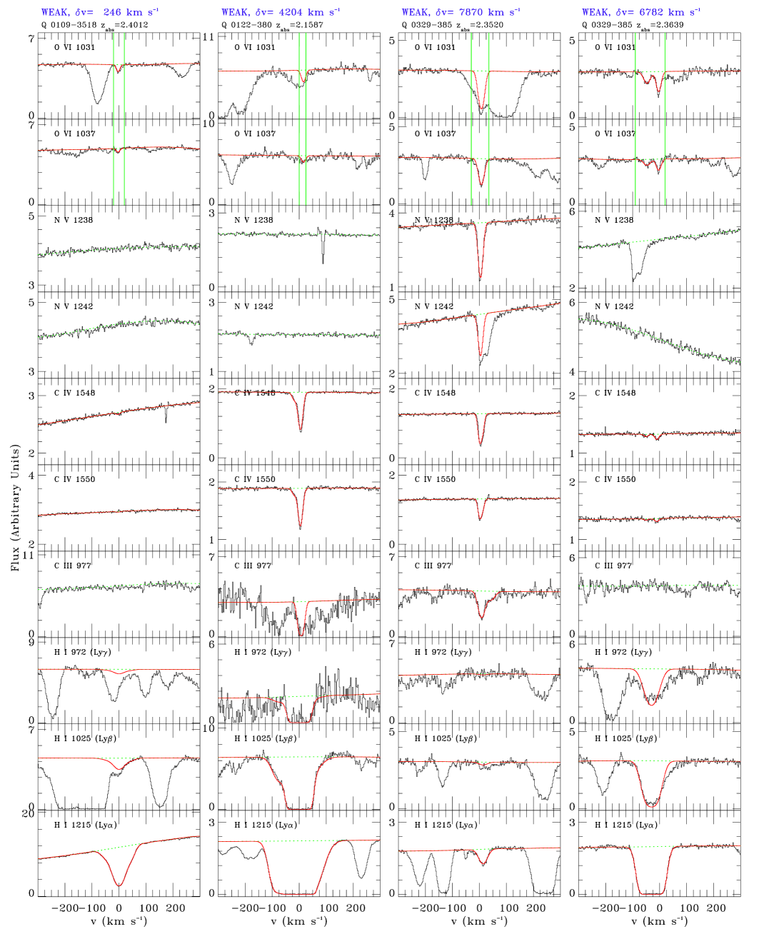
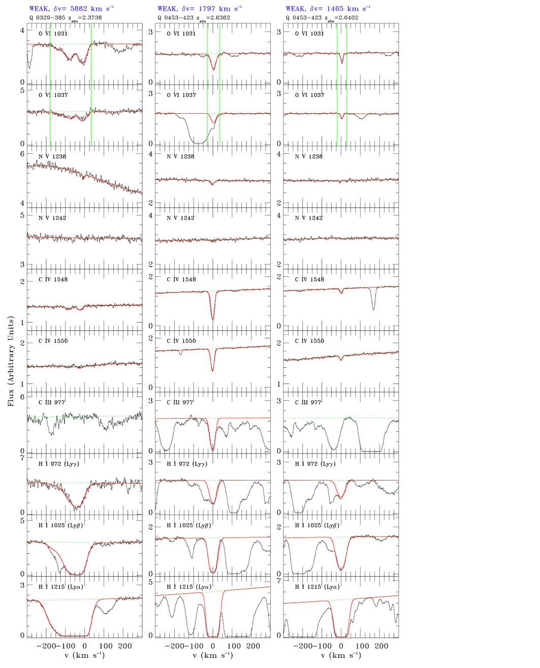
Figure 1: (cont.)

We used the VPFIT software package to determine the column densities, line widths, and central velocities of the O vi components in each system. The number of components to be fit was usually self-evident from inspection of the line profiles, but in case of doubt we used the minimum number of components necessary. Our sample of 35 O vi systems comprises 101 components. We also fit, when possible, the H i, N v, C iii, and C iv absorption, independently of the O vi fits, i.e. we did not fix any component velocity centroids or line widths when fitting the various ions. In the case of the H i lines, we simultaneously fit Ly$\alpha$ with whichever of Ly$\beta$, Ly$\gamma$, and Ly$\delta$ were unblended. The total column densities in each ion in each system were obtained by summing the component column densities, with the individual column density errors added in quadrature to produce the overall error estimate. All the Voigt profile fits are included in Figure 1, which shows the absorption-line spectra for each system in our sample. The total column density of each high ion and of H i in each system is given in Table 1. The detailed results of the component fits to O vi, N v, C iv, and H i in the weak sample are given in Tables 2 and 3. All velocities in Tables 2 and 3 are given on a scale relative to the system redshift $z_{\rm abs}$.

In addition to the component fits, we measured the total column densities in each system using the apparent optical depth (AOD) method of Savage & Sembach (1991). This method has the advantage of requiring no assumptions about the component structure: it simply requires a choice of minimum and maximum velocities for the integration. It will return accurate column densities so long as saturated structure is not present. Whereas saturation is obvious if resolved, because the flux goes to zero, unresolved saturation can be difficult to detect. In the case of a non-detection of C iv or N v, we measured the (null) equivalent width in this ion over the velocity range in which O vi is detected, and found the 3$\sigma$ error on this measurement. We then converted this maximum allowed equivalent width into a column density limit using a linear curve-of-growth. For example, if the equivalent width measurement was 0$\pm$10 mÅ, we derived a 3$\sigma$ column density limit $N_{\rm lim}$ using ${\rm EW_{lim}}$=30 mÅ and the relation $N_{\rm lim}=1.13\times 10^{17}{\rm EW_{lim}}/\lambda^{2}f$ (with $N_{\rm lim}$ in cm^-2 and $\lambda$ in Å). Atomic data were taken from Morton (2003).

In many of the strong absorbers, partial coverage of the continuum source is present. Indeed, we use this as a criterion to classify an absorber as intrinsic. Partial coverage is indicated by a similar velocity structure in the two members of a doublet, but with inconsistent optical depths in each ion. In the case of partial coverage the equation $F(v)=F_{0}e^{-\tau(v)}$ is no longer valid (e.g. Hamann & Ferland, 1999), and a velocity-dependent coverage fraction must be introduced. For these cases, the column density derived from an AOD integration should be considered as a lower limit.

3 Results

In this section we present a discussion of the overall properties of the population of proximate O vi absorbers at $z$=2–3. Although we discuss ionization processes, a detailed discussion of the physical conditions in the individual systems that make up our sample is beyond the scope of this paper. Some of the systems in our sample are discussed in more detail elsewhere. These include the proximate absorbers toward HE 2347-4342 (Fechner, Baade, & Reimers, 2004), and toward HE 1158-1843, PKS 0329-255, and Q0453-423 (D’Odorico et al., 2004).

3.1 Location of absorbers in velocity space

The number of proximate O vi absorption line systems seen in each quasar spectrum varies between zero and five. There are two quasar spectra in our sample without O vi absorption detected within 8 000 km s^-1 of $z_{\rm qso}$: HE 2217-2818 ($z_{\rm qso}$=2.41) and Q0002-422 ($z_{\rm qso}$=2.77). There are two quasars with five proximate O vi absorbers in their spectra: PKS 0237-23 ($z_{\rm qso}$=2.233) and HE 1341-1020 ($z_{\rm qso}$=2.135). To illustrate the location in velocity space of the absorbers, we show in Figure 2 the velocity displacement of all absorbers, strong and weak, for each quasar. Over the whole sample (16 spectra) we find a mean of 0.6 strong proximate O vi systems per sight line, and 1.6 weak proximate O vi absorbers per sight line. However, the O vi sample is incomplete, because of regions where O vi systems are missed due to blending by the Ly$\alpha$ forest. As we show in §3.7, when we calculate the corrected redshift path for the O vi search, our estimated O vi completeness is 84% down to a limiting equivalent width of 8 mÅ.

As a useful gauge of the velocity interval in which we expect to see proximity effects, we can derive the distance from each quasar at which the flux of extragalactic background (EGB) radiation equals the flux of quasar radiation, i.e. we can derive an estimate of the size of the quasar sphere-of-influence. The monochromatic quasar ionizing luminosities at the Lyman Limit have been derived for ten of the sixteen quasars by Rollinde et al. (2005), who calculated $L_{912}$ by extrapolating the QSO $B$-magnitudes assuming a spectral slope of $\alpha$=$-$0.5 (where $F_{\lambda}\!\sim\!\lambda^{\alpha}$). The EGB flux at the Lyman Limit at $z$=2.5 has been calculated to be $F_{\rm EGB}\!\approx\!6\!\times\!10^{-21}$ erg cm^-2 s^-1 Hz^-1 (Haardt & Madau, 1996, corresponding to log $J_{\nu}$=$-$21.3 erg cm^-2 s^-1 Hz^-1 sr^-1; the values for the $z$=2 and 3 cases are not significantly different). The distance $D$ at which $F_{\rm QSO}$=$F_{\rm EGB}$ is given by $D$=$\sqrt{(}L_{912}/4\pi F_{EGB}$). In the case where the velocities are Hubble flow-dominated, we can convert our calculated values of $D$ to velocity displacement from the quasar, using a value for the Hubble parameter calculated at the redshift of each quasar using $H^{2}(z)=H^{2}_{0}[\Omega_{\rm M}(1+z)^{3}+\Omega_{\Lambda}]$. With our adopted cosmology, $H(2.5)$=246 km s^-1 Mpc^-1. These results are shown in Table 4, and are included in Figure 2, where it can be seen that if the velocity displacements from the QSO are due to the Hubble flow, then the proximity effect should only extend to $\sim$1 000–2 500 km s^-1. While peculiar velocities are to be expected, this is still a useful order-of-magnitude estimate for the size of the quasars’ ionizing sphere-of-influence.

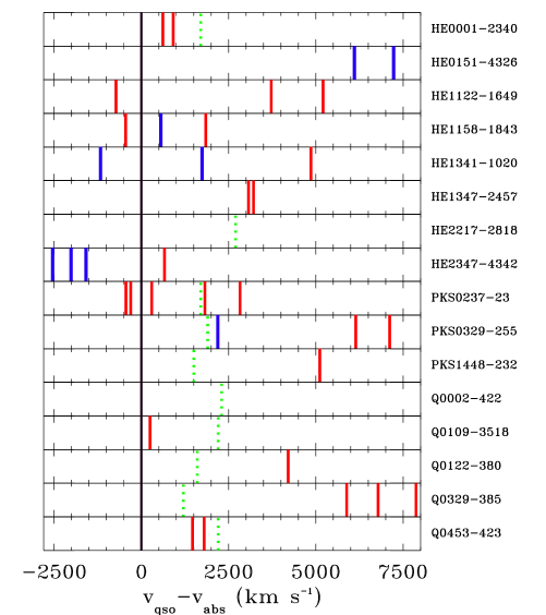
Figure 2: Graphical display of the location in velocity space of the O vi absorbers in this study, relative to their background quasar. Weak absorbers are shown in red, and strong absorbers in blue. The location of $\delta v$=0, i.e. $z_{\rm abs}$=$z_{\rm qso}$, is shown with a solid black line. Negative values for $v_{\rm qso}\!-\!v_{\rm abs}$ imply the absorber is approaching the quasar. Dashed green lines show the velocity at which $F_{\rm QSO}$=$F_{\rm EGB}$ assuming Hubble flow (see text).

Table 4: Size of quasar spheres-of-influence at 912 Å.

QSO	log $L_{912}$	$D$	$\delta v$
	(erg s-1 Hz-1)	(Mpc)	(km s-1)
HE 0001-2340	31.65	7.7	1700
HE 2217-2818	31.99	11.4	2600
PKS 0237-23	31.67	7.8	1700
PKS 0329-255	31.58	7.1	1800
PKS 1448-232	31.53	6.7	1400
Q 0002-422	31.72	8.3	2200
Q 0109-3518	31.82	9.3	2200
Q 0122-380	31.63	7.5	1600
Q 0329-385	31.28	5.0	1100
Q 0453-423	31.71	8.2	2100

3.2 Presence of other ions

The presence and strength of absorption in other ionic species in the proximate O vi absorbers provides important information on the ionization conditions. H i absorption is detected in each of the 35 O vi systems, always in Ly$\alpha$ and occasionally up to Ly$\delta$. Higher-order Lyman lines may also be present, but they lie deep in the Ly$\alpha$ forest where blending and low signal-to-noise aggravate the search for detections. All but two of the O vi systems show C iv detections (the exceptions are the absorbers at $z_{\rm abs}$=2.2378 toward PKS 0237-23 and $z_{\rm abs}$=2.6610 toward PKS 0329-255, both of which are weak O vi systems with low O vi column densities). 9/9 strong O vi systems contain N v, whereas 9/26 weak O vi systems contain N v. Therefore while the presence of N v is a feature of all strong systems, it does not imply that an O vi system is strong. Finally, C iii absorption is seen in 13/26 weak systems, and 7/9 strong systems. However, because C iii $\lambda$977 lies in the Ly$\alpha$ forest, it is often blended and hence not detectable even if present, so these fractions should be treated as lower limits.

3.3 O vi system column densities

A plot of the total O vi column densities in each absorber versus proximity (Figure 3, top panel) shows the distinction between the strong and weak populations. The strong population all show log $N\!\ga\!15.0$ and are(with two exceptions) clustered around $z_{\rm abs}$=$z_{\rm qso}$, whereas the weak population lies between the detection limit of log $N\!\approx\!12.80$ (corresponding to a limiting equivalent width of 8 mÅ) and 14.5. Once the strong systems have been removed, the underlying weak population shows no dependence of $N$(O vi) with proximity to the quasar. To investigate this further, we split the sample into O vi absorbers at $\delta v\!<\!2\,000$ km s^-1 and those at $2\,000\!<\!\delta v\!<\!8\,000$ km s^-1. This division is motivated by an observed enhancement in d$N$/d$z$ below 2 000 km s^-1 (§3.7), as well as this representing the expected size of the proximity zone (§3.1). A two-sided Kolmogorov-Smirnov (K-S) test shows that the probability that the distribution of log $N$(O vi) for absorbers at $<$2 000 km s^-1 is different from those at $>$2 000 km s^-1 is only 17%. There is also no clear correlation between the quasar redshift and the total O vi column, as shown in the lower panel of Figure 3. We do note that the ratio of weak systems to strong systems changes from 6.3 (19/3) at $z\!<\!2.5$ to 1.2 (7/6) at $z\!>\!2.5$, but the statistics are too small for us to investigate this further.

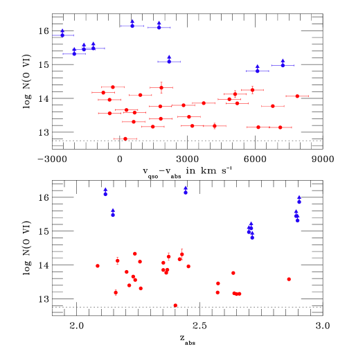
Figure 3: Scatter plots comparing the integrated column density (over all components) of the O vi absorbers with their proximity to the background quasar $\delta v\equiv v_{\rm qso}\!-\!v_{\rm abs}$ and with their redshift $z_{\rm abs}$. An error of 500 km s^-1 in $z_{\rm qso}$ is assumed. Strong absorbers are shown in blue (lower limits), with weak absorbers in red. The distinction between the weak and strong populations is evident. The dashed line shows the detection limit. Among the weak absorbers there is no correlation between $N$(O vi) and $\delta v$, or between $N$(O vi) and $z$.

3.4 O vi component column densities and $b$-values

Proximity effects may occur at the component level, as well as the system level. To investigate this, we compare in Figure 4 the component properties returned by VPFIT (column densities and line widths) of the weak O vi absorbers with $\delta v$. We include for comparison the O vi components from the intervening sample of BH05. As with the system column densities, there is no trend for the component O vi column densities to correlate with proximity to the quasar.

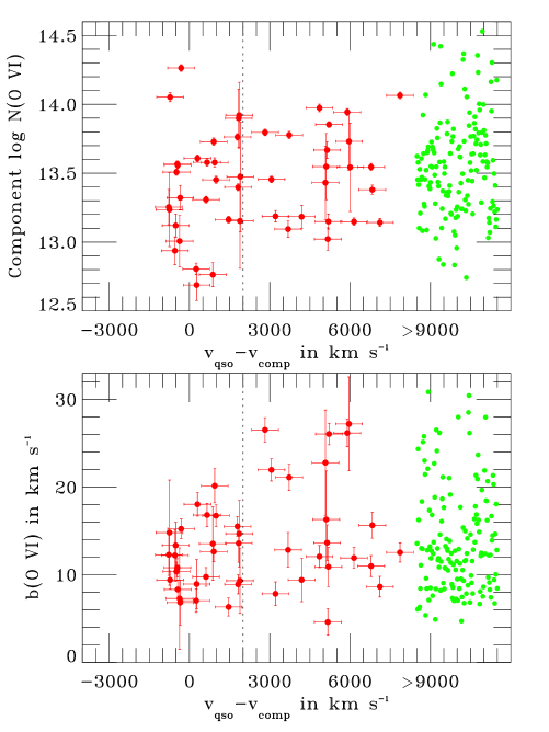
Figure 4: Scatter plots comparing the column densities and line widths of the O vi components with their proximity to the background quasar. The errors shown are returned by the VPFIT profile-fitting code. Included in green is the BH05 sample of intervening O vi components at $z$=2–2.5, plotted for convenience at $\delta v>9\,000$ km s^-1, with arbitrary shifts in the x-direction applied for clarity. Two proximate components with $b$=34$\pm$14 and 45$\pm$18 km s^-1 are not shown because of their large errors.

The distributions of log $N$ and $b$ for the O vi components in our sample are shown in Figure 5. We include the following component distributions as separate curves: the components at $\delta v\!<\!2\,000$ km s^-1, those at $2\,000\!<\!\delta v\!<\!8\,000$ km s^-1, and the intervening absorbers from BH05. A two-sided K-S test finds the probability that the log $N$ distributions for the samples at $<$2 000 km s^-1 and 2 000–8 000 km s^-1 are different (i.e. drawn from distinct parent populations) is only 23%. Comparing the $\delta v\!<\!2\,000$ km s^-1 components to the intervening sample, we do not find any difference valid at more than the 1.0$\sigma$ level, with the intervening sample showing a median log $N$(O vi) of 13.54, and the $\delta v\!<\!2\,000$ km s^-1 sample showing a median of 13.45. This is an important result considering the intervening sample was measured independently in BH05, not in this analysis.

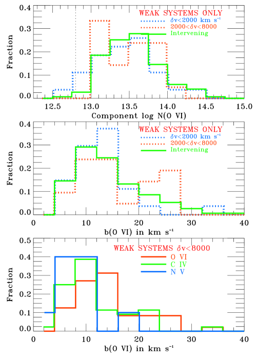
Figure 5: Top two panels: normalized column density- and line width distributions of the proximate O vi components at $\delta v\!<\!2\,000$ km s^-1, at $2\,000\!<\!\delta v\!<\!8\,000$ km s^-1, and in the intervening sample. No statistically significant differences are found, with the exception of a slight excess of systems with $b$=20–30 km s^-1 in the weak sample in the 2 000–8 000 km s^-1 bin. The bottom panel compares the line width distributions for O vi, C iv, and N v in the weak, proximate sample.

Turning to the component line widths, we find that among the proximate weak sample, 29 out of 48 components (60%) are narrow ($b\!\leq\!14$ km s^-1). Comparing the $b$-value distributions, we find that the probability that the population at $\delta v<2\,000$ km s^-1 is different from the intervening distribution is less than 50 per cent. The median $b$-value in the intervening sample is 12.7 km s^-1; in the sample at $\delta v\!<\!2\,000$ km s^-1, it is 12.3 km s^-1. However, an excess of systems with $b$=20–30 km s^-1 is observed for components in the 2 000–8 000 km s^-1 range, as can be seen in the lower panel of Figure 4.

Finally, we compare the line width distribution of the O vi components in the weak proximate sample with the C iv and N v line width distributions (in the same sample). The line widths of C iv and N v distribute differently than those of O vi, without the strong tail extending between 10 and 25 km s^-1 seen in the O vi distribution. 77% of C iv components and 90% of N v components show $b\!<\!14$ km s^-1. These differences indicate that it cannot be assumed that the C iv, N v, and O vi arise in the same volumes of gas.

In summary, among the weak O vi absorbers at $z$=2–3, there is no compelling evidence for any difference in the column density and line width distributions between the intervening and proximate O vi populations, but within the proximate sample, the O vi line widths distribute differently than those of N v and C iv.

3.5 H i column density

The median and standard deviation of the logarithmic H i column density in the weak proximate O vi sample is log $N$(H i)=14.66$\pm$0.95, with a total range covered in log $N$(H i) of over four decades. The H i/O vi ratio (integrated over all components in each system) varies enormously, taking values between 0.02 and 1500. In Figure 6 (top panel) we plot the H i/O vi column density ratio against the H i column density. Within both the strong and weak samples, a trend is evident in which H i/O vi rises with increasing $N$(H i). However, the two populations are clearly distinct, in that the weak systems show much higher H i/O vi ratios at a given $N$(H i). The clear segregation of the weak and strong systems on this plot supports our contention that they represent two separate populations.

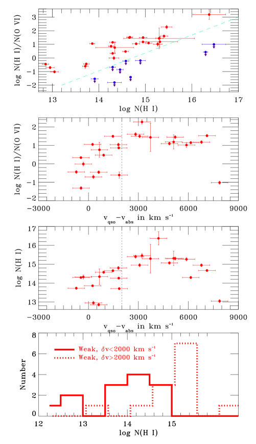
Figure 6: Analysis of $N$(H i) and the H i/O vi ratio in the proximate O vi sample. The column densities are integrated over all components in each absorber. In the top panel, a dashed line delineates the locations of the strong (blue) and weak (red) samples in a plot of H i/O vi vs H i. In the central two panels we show that both $N$(H i) and H i/O vi show a dependence on proximity. The bottom panel shows the histogram of $N$(H i) for the weak O vi absorbers, split into two sub-samples: those at $\delta v\!<\!2\,000$ and $\delta v\!>\!2\,000$ km s^-1. A significant difference exists between these two histograms, with the absorbers closer in velocity to the quasar showing lower $N$(H i).

In the lower panels of Figure 6, we explore whether the H i column density in the weak proximate sample depends on $\delta v$. We find that $N$(H i) distributes very differently at $\delta v\!<\!2\,000$ km s^-1 than at $\delta v\!>\!2\,000$ km s^-1. The $N$(H i) distribution for the $\delta v\!>\!2\,000$ km s^-1 sub-sample is strongly clustered around log $N$(H i)$\approx$15, whereas the distribution for the $\delta v<2\,000$ km s^-1 sub-sample is centered near log $N$(H i)$\approx$14 (see bottom panel). A K-S test shows the two distributions differ at the 99.97% level. Consequently, there is also a difference in the mean H i/O vi ratio above and below 2 000 km s^-1, but this is due to the proximity effect in $N$(H i), not in $N$(O vi), which shows no correlation with proximity to the quasar. The finding that $N$(H i) correlates with $\delta v$ has an important implication: it implies that $\delta v$ does correlate with physical distance to the quasar. If $\delta v$ was dominated by peculiar motions rather than Hubble flow, and so was uncorrelated to physical proximity to the quasar, then the two $N$(H i) distributions shown in the bottom panel of Figure 6 would not be distinct. The fact that they are so different allows us to make the general assumption that proximity in velocity does imply proximity in distance.

3.6 C iv and N v column densities

The logarithmic C iv column densities in the proximate O vi sample cover over 2 dex, with a median value and standard deviation of log $N$(C iv)=12.64$\pm$0.60. N v is detected in nine weak absorbers, with log $N$(N v) between 11.54 and 13.60. Comparisons between the C iv column density and $\delta v$, and between N v column density and $\delta v$, as well as the dependence of the high-ion column density ratios with $\delta v$, are presented in Figure 7. In a similar fashion to H i, $N$(C iv) in the weak O vi absorbers depends strongly on $\delta v$, with the absorbers at $\delta v\!<\!2\,000$ km s^-1 showing column densities clustered around log $N$(C iv)$\approx$12.4, and those at $\delta v\!>\!2\,000$ km s^-1 showing values centered at log $N$(C iv)$\approx$13.3. A two-sided K-S test shows that the $N$(C iv) distributions in the two velocity intervals differ at a significance level of 93%. This leads to a difference in the mean C iv/O vi ratio between the two velocity bins, with lower ratios at lower velocity. There is no indication that either $N$(N v) or N v/O vi depends on $\delta v$, though the smaller sample size of N v (because of the non-detections) prevents us from making statistically meaningful conclusions.

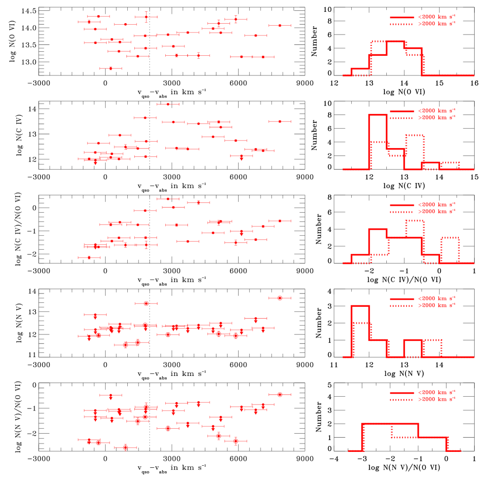
Figure 7: Dependence of $N$(O vi), $N$(C iv), $N$(C iv)/$N$(O vi), $N$(N v), and $N$(N v)/$N$(O vi) on $\delta v$, for the weak proximate O vi sample. Downward-pointing arrows denote non-detections. The right column shows the histograms of each quantity plotted on the left, split into sub-samples at $\delta v\!<\!2\,000$ and $>$2 000 km s^-1 from the quasar. In the lower two panels, the nine N v detections are shown with open circles to distinguish them from the non-detections. Only detections are included in forming the histograms. Whereas there is no discernable effect for $N$(O vi) to depend on $\delta v$, $N$(C iv) distributes very differently at $<$2 000 than at $>$2 000 km s^-1. The N v samples are too small to draw conclusions about whether $N$(N v) depends on $\delta v$.

In order to study the high-ion velocity structure more closely, we present in Figures 8a and 8b apparent column density profiles as a function of velocity, for each weak proximate O vi absorber. The apparent column density per unit velocity in units of ions cm^-2 (km s^-1)^-1 is given by $N_{a}(v)=3.768\times 10^{14}\tau_{a}(v)/f\lambda$ (Savage & Sembach, 1991), where $\lambda$ is the transition rest wavelength in Å, $f$ is the oscillator strength (taken from Morton, 2003), and $\tau_{a}(v)$ is defined in §2.2. These figures allow the O vi, C iv, H i, and (in the nine cases where present) N v profiles to be closely compared. Note that for H i, we plot the apparent column density profile of our best-fit model to the Lyman series absorption lines, because several lines are used to derive our best-fit model. For the high ions, the actual data from one of the two doublet lines are shown, rather than the model.

In 11/24 absorbers where both O vi and C iv are detected, the profiles are similar enough to suggest co-spatiality of the ions C⁺³ and O⁺⁵. In the remaining 13 cases there are significant differences in the line profiles, indicating that O vi and C iv trace different gas phases. Here a ‘significant difference’ is either a centroid offset of $>$10 km s^-1, or a case where $b$(C iv)$<$ $b$(O vi), for which there is no single-phase solution [since an oxygen atom is heavier than a carbon atom, $b$(O vi) must be less than $b$(C iv) for lines arising in the same gas]. In only one of the nine cases with N v, its profile is similar in centroid and width to the O vi. However, detailed comparisons of the N v and O vi profiles are complicated by the fact that low-optical depth N v absorption is lost in the noise, even in this high-quality dataset, so we do not read into this result any further. Most significantly, offsets of order 10–30 km s^-1 between the centroid of the H i absorption and the centroid of O vi absorption are seen in 14/26 weak proximate cases. These offsets are highly important, since they imply that the H⁰ atoms do not live in the same volume of gas as the O⁺⁵ ions in at least half of the weak O vi absorbers. In other words, at least half of the weak O vi systems are multi-phase. Consequently, it is not possible to derive a metallicity estimate in these multi-phase cases from the O vi/H i ratio, even with an ionization correction, and single-phase photoionization models cannot be applied. The dangers of treating multi-phase quasar absorbers as single-phase have been pointed out before (Giroux, Sutherland, & Shull, 1994; Reimers et al., 2001).

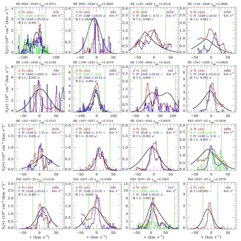
Figure 8: High-ion and H i apparent column density profiles for each weak proximate O vi absorber. The C iv (blue), H i (black), and N v (green, where present) profiles have been scaled to allow their shape to be compared with O vi. For the high ions the AOD profiles are formed from the data themselves. For H i, we show the AOD profile of the best-fit model to the Lyman series absorption lines. The green vertical lines show the velocity range over which the AOD measurement is made. Annotated on the top-right of each panel is the proximity to the quasar. In cases where the O vi and C iv profiles show similar line centers and line widths, we add a tick to the C iv label. In cases where the O vi and H i profiles show similar velocity centroids (but not necessarily the same width), we add a tick mark to the H i label. Cross marks next to the C iv and H i labels indicate significant differences between the profiles of these ions and O vi, e.g. centroid offsets of $>$10 km s^-1, indicating that the lines do not form in the same phase of gas as the O vi.

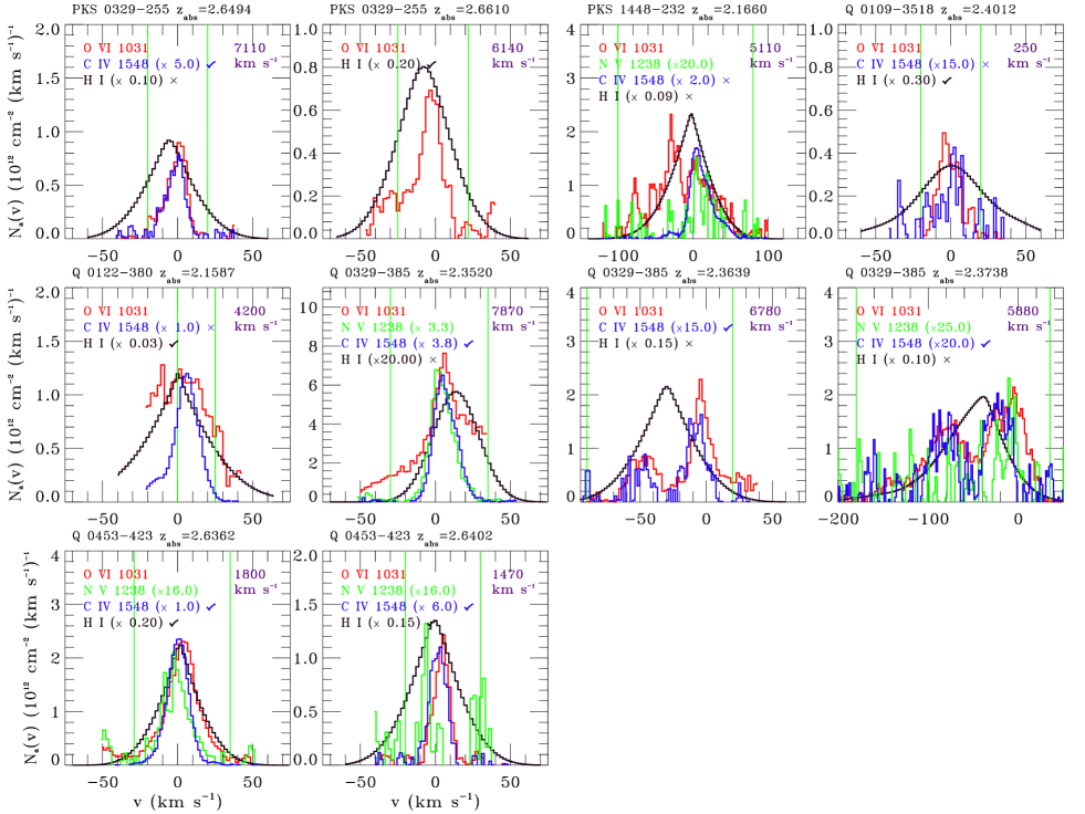
Figure 8: (continued). High-ion and H i apparent column density profiles in the weak O vi absorbers.

3.7 Calculation of d$N$/d$z$ for proximate O vi

In this section we derive the incidence of proximate O vi absorption, in terms of the traditional d$N$/d$z$, and also in terms of the number of absorbers detected per 2 000 km s^-1 interval in $\delta v$. Note that because we are working at $z\!\gg\!0$, relativistic effects cause the relationship between velocity and redshift intervals to be d$v\!\approx\!c$ d$z$/(1+$z$). Before calculating the incidence of proximate O vi absorption, we correct the redshift path for blending with the Ly$\alpha$ forest, since O vi is only identifiable in unblended regions of the spectrum. To estimate the number of O vi absorbers that were missed due to Ly$\alpha$ forest contamination, we looked for C iv absorbers within 8 000 km s^-1 of $z_{\rm qso}$ in which the accompanying O vi is blended, and found five. These are listed in Table 5. This method should provide a good estimate for the O vi incompleteness, since firstly O vi is detected in all proximate C iv absorbers in which the O vi data are unblended, and secondly C iv is unblended by the Ly$\alpha$ forest, so no C iv systems should be missed down to a limiting equivalent width of $\approx$2 mÅ. The limiting equivalent width for the C iv search is smaller than the limiting equivalent width for the O vi search, because C iv lies in a higher S/N region of the spectrum.

Table 5: Proximate C iv with blended O vi

QSO	$z_{\rm qso}$	$z_{\rm abs}$	$\delta v$ (km s-1)
HE 0001-2340	2.2670	2.1870	7530
HE 0151-4326	2.7890	2.6956	7580
HE 1341-1020	2.1350	2.1065	2750
HE 2347-4342	2.8710	2.8781	$-$550
Q 0122-380	2.2030	2.1472	5320

The total redshift path within 8 000 km s^-1 of sixteen quasars (at $\langle z_{\rm qso}\rangle$=2.44) is 1.48. Because there are five ‘missing’ O vi systems, we estimate our O vi completeness to be 35/(35+5)=84%, implying that a path equal to 0.25 is blended near O vi, so that the corrected redshift interval for the proximate O vi search is 1.24. In this path 26 weak systems (comprising 48 components) are detected. so overall d$N$/d$z$ of weak O vi systems at $\delta v\!<\!8\,000$ km s^-1 is 21$\pm$5, where the errors on the counts are assumed to be Poissonian. However, this is an average value, and when we break down the absorbers into those at $\delta v\!<\!2\,000$ and those at 2 000–8 000 km s^-1, we find a marked change in the incidence: d$N$/d$z$ trebles within 2 000 km s^-1, from 14$\pm$4 to 42$\pm$12. When counting components rather than systems, a similar increase in the incidence is observed within 2 000 km s^-1 of $z_{\rm qso}$. These results are shown in Figure 9, and are also summarized in Table 6. Note how the intervening incidence of BH05 is recovered in the range 2 000–8 000 km s^-1.

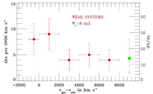
Figure 9: Number of weak O vi absorbers as a function of proximity to the quasar. Plotted are the number of O vi systems per 2 000 km s^-1 bin of $\delta v$ over our sample of sixteen quasars. The corresponding values of d$N$/d$z$ are shown on the right, corrected for the blended redshift path. The errors on the counts are assumed to be Poissonian; plotted are the 1$\sigma$ errors. We use a smaller bin for the range $-$1 000 to 0 km s^-1; these absorbers lie in front of the quasar and so are included in the 0–2 000 km s^-1 bin in our final d$N$/d$z$ calculations. The incidence of intervening O vi systems is shown as the green data point; there is no significant difference in d$N$/d$z$ between the absorbers at 2 000–8 000 km s^-1 and the intervening sample.

Table 6: Weak O vi absorbers at $z$=2–3: Summary of d$N$/d$z$ statistics (8 mÅ sensitivity)

Category	$|\delta v|\!<\!2\,000$	$2\,000\!<\!\delta v\!<\!8\,000^{\rm a}$	Intervening
Systems	42$\pm$12	14$\pm$4	14$\pm$2
Components	87$\pm$17	23$\pm$5	35$\pm$6

3.8 Comparison of $z\approx 2.5$ and $z\approx 0$ absorbers

A considerable amount of work has been invested in studying O vi in the low-redshift IGM using the FUSE and HST orbiting observatories (Bergeron et al., 1994; Burles & Tytler, 1996; Tripp et al., 1996; Tripp, Savage, & Jenkins, 2000; Savage et al., 2002; Sembach et al., 2004; Richter et al., 2004; Prochaska et al., 2004; Danforth & Shull, 2005, 2008; Lehner et al., 2006; Tripp et al., 2008; Cooksey et al., 2008; Thom & Chen, 2008a, b). By comparing our results obtained from proximate O vi absorbers at $z$=2–3 with the $z\!\approx\!0$ results, we can search for evolution of the highly ionized gas content of the Universe. Since the intensity of the extragalactic UV background rises with redshift (Haardt & Madau, 1996), one might expect to see higher photoionized O vi column densities at higher redshift. Simultaneously, the fraction of baryons in warm-hot gas is predicted to decrease with increasing redshift (Davé et al., 2001), since at early cosmic epochs there has not been adequate time for gas to accrete and virialize into dark matter-dominated potential wells.

Based on an analysis of low-redshift ($0.15\!<\!z\!<\!0.5$) O vi absorption line systems and with a sensitivity limit of $W_{\rm r}\!>\!30$ mÅ, Tripp et al. (2008) report that d$N$/d$z$ is enhanced by a factor of $\approx$3 at velocities $<$2 500 km s^-1 from the quasar compared to the intervening sample, with d$N$(O vi)/d$z$=16${}^{+3}_{-2}$ for the intervening systems and d$N$(O vi)/d$z$=51${}^{+21}_{-15}$ for those at $\delta v<2\,500$ km s^-1. Our result for weak O vi systems at $z$=2–3 with $W_{\rm r}\!>\!30$ mÅ and $\delta v\!<\!2\,000$ km s^-1 is d$N$/d$z$ is 32$\pm$10, lower than the low-redshift result by a factor of $\approx$1.6. However, comparing the high- and low-redshift results for d$N$/d$z$ can be misleading, because redshift has a highly non-linear relationship with spatial dimensions, that depends on cosmology. With our adopted cosmology, then in the interval $z$=0.15 to $z$=0.5, d$x$(Gpc)=3.63 d$z$, whereas for the interval $z$=2 to $z$=3, d$x$(Gpc)=1.22 d$z$, where d$x$ is the comoving radial distance, and where we have used the online cosmology calculator of Wright (2006). Correcting for these factors to calculate the number density of weak O vi absorbers per unit co-moving distance, a better indicator of the space density of O vi, we derive the results listed in Table 7. Here we see evidence that the space density of O vi absorbers increases with redshift, by a factor of two between $z$=0.15–0.5 and $z$=2–3. This increase is observed independently for both the proximate and intervening absorbers.

Table 7: d$N$(O vi)/d$x$ statistics (30 mÅ sensitivity)

Category	Sample	$z$=0–0.5	$z$=2–3
		(Gpc-1)	(Gpc-1)
Systems	Proximate ($\delta v\!<\!2\,000$)	14${}^{+6}_{-4}$	26$\pm$8
	Intervening ($\delta v\!>\!5\,000$)	4$\pm$1	8$\pm$2
Components	Proximate ($\delta v\!<\!2\,000$)	30${}^{+8}_{-6}$	71$\pm$14
	Intervening ($\delta v\!>\!5\,000$)	6$\pm$1	21$\pm$3c

4 Discussion

The BAL, mini-BAL, and intrinsic systems, which together we classify as strong systems based on their fully saturated O vi absorption, strong accompanying O vi and C iv absorption, and frequent evidence for partial coverage, are well-understood as being formed in either QSO-driven outflows or inflows in the immediate vicinity of the AGN central engine (see review by Hamann & Ferland, 1999). Here we focus on the weak (narrow) proximate systems, which represent a separate population. Is there any evidence that these weak systems are directly photoionized by the quasar?

We report two results that address this question, though their interpretation is not straightforward. First, in our sample of proximate O vi absorbers at $z$=2–3, there is an enhancement by a factor of three in the incidence d$N$/d$z$ of weak O vi absorbers within 2 000 km s^-1 of the quasar versus those in the interval 2 000 to 8 000 km s^-1. A similar enhancement is seen near low-redshift quasars (Tripp et al., 2008). While at face value this could be interpreted as a proximity effect, in which quasars preferentially ionize nearby clouds more often than they photoionize more distant clouds, this is not the only explanation. The enhancement in d$N$/d$z$ could also be explained by an over-density of galaxies near quasars, and where the O vi absorbers are located in the gaseous halos of these galaxies (Young, Sargent, & Boksenberg, 1982). It is well-known that quasars are preferentially formed in cluster environments, particularly at high redshift (Croom et al., 2005; Shen et al., 2007). This idea is supported by the observation that the internal properties of the weak O vi absorbers are not dependent on redshift or proximity to the quasar.

Second, there are statistically significant differences between the H i/O vi and C iv/O vi ratios measured in the weak O vi populations above and below 2 000 km s^-1, with the weak absorbers at $\delta v\!<\!2\,000$ km s^-1 showing a median H i/O vi ratio lower by a factor of $\approx$10, and a median C iv/O vi ratio lower by a factor of $\approx$7 than those at $2\,000\!<\!\delta v\!<\!8\,000$ km s^-1. Again, at face value, these results could be interpreted as proximity effects, in which gas closer to the quasar shows a higher ionization level than intervening gas. However, closer inspection finds that while $N$(H i) and $N$(C iv) show a tendency to decrease as $\delta v$ decreases, $N$(O vi) is uncorrelated with $\delta v$, i.e. it is the behaviour of $N$(H i) and $N$(C iv) alone that is driving the trends seen in the column density ratios, not the behaviour of $N$(O vi). Importantly, the H i and C iv proximity effects imply that proximity in velocity does correlate with proximity in distance, which supports the idea that the velocities of the weak absorbers are dominated by the Hubble flow.

Because O vi-H i-C iv velocity centroid offsets are observed directly in $\approx$50 per cent of the weak systems, single-phase photoionization models for the O vi, C iv, and H i are inadequate for at least half the absorbers in our sample. Indeed, the non-dependence of $N$(O vi) on proximity casts doubt on whether photoionization by the background QSO creates the O vi at all. Photoionization by nearby stellar sources of radiation is also unlikely, since such sources do not emit sufficient fluxes of photons above 54 eV (the He ii ionization edge) to produce the observed quantities of O vi. We cannot rule out photoionization by the quasar in every individual case, for example the absorber at $z$=2.4183 toward HE 1122-1649, which shows strong O vi but barely detectable C iv, as do several proximate O vi absorbers reported by Gonçalves et al. (2008). Nonetheless, $N$(O vi) does not depend on proximity in the way that $N$(H i) and $N$(C iv) do. Thus we infer that the sizes of spheres-of-influence around quasars, which are implied the shapes of Gunn-Petersen troughs (Zheng & Davidsen, 1995; Smette et al., 2002), and from studies of proximate absorption in lower ionization species, such as Mg ii (Vanden Berk et al., 2008; Wild et al., 2008) and C iv (Foltz et al., 1986; Vestergaard, 2003; Nestor et al., 2008), are dependent on photon energy, and the presence of a sphere of photons at energies above 113.9 eV (capable of ionizing O⁺⁴ to O⁺⁵) has yet to be demonstrated.

Thus we turn to collisional ionization models. Since the line widths of a significant fraction ($\approx$60%) of the components in the weak O vi absorbers are low enough ($b\!<\!14$ km s^-1) to imply gas temperatures below 188 000 K, collisional ionization equilibrium can be ruled out, because essentially no O vi is produced in gas in CIE at these temperatures (Sutherland & Dopita, 1993; Gnat & Sternberg, 2007). Indeed, the narrow line widths of many intergalactic O vi absorbers at $z\!\approx\!2$ have led various authors to conclude that photoionization is the origin mechanism (Carswell et al., 2002; Bergeron et al., 2002; Levshakov et al., 2003; Bergeron & Herbert-Fort, 2005; Reimers et al., 2006; Lopez et al., 2007). However, non-equilibrium collisional ionization models cannot be ruled out so easily. Indeed one expects that collisionally ionized gas at ‘coronal’ temperatures of a few $\times 10^{5}$ K, where O vi is formed through collisions, will be in a non-equilibrium state. This is because the peak of the interstellar cooling curve exists at these temperatures, and so the cooling timescales are short. When the cooling times are shorter than the recombination timescales, ‘frozen-in’ ionization can result at temperatures well below those at which the ions exist in equilibrium (Kafatos, 1973; Shapiro & Moore, 1976; Edgar & Chevalier, 1986), provided that there is a source of $\sim 10^{6}$ K gas in the first place.

There are at least two physical reasons why collisionally-ionized, million-degree regions of interstellar and intergalactic gas could arise in the high-$z$ Universe. The first is the (hot-mode) accretion and shock heating of gas falling into potential wells (Birnboim & Dekel, 2003; Kereš et al., 2005; Dekel & Birnboim, 2006), a process which is incorporated into cosmological hydrodynamical simulations (Cen & Ostriker, 1999; Davé et al., 2001; Fang & Bryan, 2003; Kang et al., 2005; Cen & Fang, 2006), and creates what is referred to as the Warm-Hot Intergalactic Medium. However, these models generically predict that the fraction of all baryons that exist in the WHIM rises from essentially zero at $z$=3 to 30–50% at $z$=0, so little WHIM is expected at the redshifts under study here. The second reason is the presence of galactic-scale outflows, which due to the energy input from supernovae are likely to contain (or even be dominated by) hot, highly ionized gas (see recent models by Oppenheimer & Davé, 2006; Fangano, Ferrara, & Richter, 2007; Kawata & Rauch, 2007; Samui, Subramanian, & Srianand, 2008). There is strong observational evidence for outflows at redshifts of $\approx$2–3 (Heckman, 2002), including blueshifted absorption in the spectra of Lyman break galaxies (Pettini et al., 2000, 2002; Shapley et al., 2003), the presence of metals in the low-density, photoionized IGM (the Ly$\alpha$ forest; e.g. Aracil et al., 2004; Aguirre et al., 2005, 2008), though see Schaye, Carswell, & Kim (2007), and the presence of super-escape velocity C iv components in the spectra of damped Ly$\alpha$ (DLA) galaxies (Fox et al., 2007b). In addition, collisionally ionized gas in galactic halos at high redshift has been seen directly through detections of O vi and N v components in DLAs (Fox et al., 2007a), albeit with much broader system velocity widths than in the proximate absorbers discussed here. O vi absorbers with lower H i column density may probe the outer reaches of such halos or ‘feedback zones’ (BH05; Simcoe et al., 2002).

We explore the ability of non-equilibrium collisional ionization models to reproduce the data in our proximate O vi sample in Figure 10, which shows the C iv/O vi vs N v/O vi ratio-ratio plane. We take the isobaric non-equilibrium model at log $T$=5.00 (consistent with the observed O vi component line widths) from Gnat & Sternberg (2007), computed using solar abundances, and then find the values of [N/O] and [C/H] that are required to reproduce the observations. The models for 0.1 and 0.01 solar absolute abundances, and for the isochoric case, predict similar values. The non-equilibrium models are not capable of reproducing the observed ratios when solar relative elemental abundances are used. However, if [N/O] takes values between $-$1.8 and 0.4, and [C/O] between $-$1.9 and 0.6, it is possible to explain the observed column densities in each weak proximate system with a non-equilibrium collisional ionization model. Note that we have not corrected these model predictions for the effect of photoionization by the extragalactic background; the model represents the pure collisional ionization case. Hybrid collisional+photo-ionization models would help in making progress in this area (see discussion in Tripp et al., 2008).

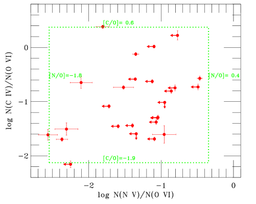
Figure 10: Comparison of predictions of non-equilibrium collisional ionization models with the observed column density ratios in our weak proximate sample. Non-detections of N v (C iv) lead to upper limits on the x- (y-) axis. We take the predictions from the isobaric non-equilibrium collisional ionization model of Gnat & Sternberg (2007) for an absorber at $T$=$10^{5}$ K (higher temperatures are ruled out by the component line widths). The model is fairly insensitive to changes in the overall abundance level, but is sensitive to non-solar relative abundances. The dashed green lines show the range of values of [N/O] and [C/O] that are required to fit the proximate data with this collisional ionization model.

5 Summary

We have presented a study of proximate ($\delta v<8\,000$ km s^-1) O vi absorbers in the spectra of sixteen quasars observed at high signal-to-noise and 6.6 km s^-1 resolution with VLT/UVES. The quasars are at redshifts between 2.14 and 2.87. We found 35 proximate O vi absorbers comprising 101 components. We used component fitting software to determine the properties of the absorption, studied the statistical properties of the sample, and addressed the ionization conditions in the gas. Our study has produced the following results.

1. Nine of the 35 O vi systems are strong, with log $N(\mbox{O\,{\sc vi}})\ga 15.0$. These absorbers all show detections of C iv and N v, and show either broad, fully saturated, mini-BAL-type O vi absorption troughs extending over tens to hundreds of km s^-1, or evidence for partial coverage in the high-ion profiles. A mean of 6.0 O vi components are seen in the strong absorbers. The strong absorbers are formed either in QSO-driven outflows or in the immediate vicinity of the quasar.

2. 26 of the 35 O vi systems are weak, and show log $N(\mbox{O\,{\sc vi}})\!<\!14.5$. These systems are narrow, with a median velocity width $\Delta v_{90}$ of 42 km s^-1. The weak systems all contain detectable H i, all but two show C iv, and 9/26 show N v. We find a mean of 1.9 O vi components per weak system. Approximately 60 per cent of these O vi components have Doppler $b$-values $<$14 km s^-1. The gas in these narrow components is constrained by the line widths to be at $T\!<\!188\,000$ K.

3. Among the weak sample there is no correlation between the O vi column density and the proximity to the quasar. This is true when using either the component-level or the system-level column densities. Two-sided K-S tests confirm that the column density distributions of the intervening and weak proximate O vi samples are statistically indistinguishable. The O vi column density also does not correlate with redshift.

4. There is a difference between the line width distributions of the O vi components versus the distributions of C iv and N v, in the weak proximate sample. The C iv and N v distributions are strongly peaked below $b$=10 km s^-1 and do not show the tail of absorbers with $b$-values between 10 and 25 km s^-1 seen in the O vi distribution.

5. There is a significantly lower $N$(H i) in the weak O vi absorbers with $\delta v\!<\!2\,000$ km s^-1 than in those with $\delta v\!>\!2\,000$ km s^-1. The difference in the median $N$(H i) between these two samples is $\sim$1.0 dex. We interpret this as a manifestation of the H i proximity effect, and it leads to a trend in which the H i/O vi ratio is lower for absorbers within 2 000 km s^-1 of the QSO than for those at higher $\delta v$. An identical trend is observed for C iv, with the median $N$(C iv) lower by $\approx$0.8 dex at $\delta v\!<\!2\,000$ km s^-1 than at $\delta v\!>\!2\,000$ km s^-1. Thus C iv and H i behave differently than O vi.

6. Apparent column density profile comparisons show that O vi and C iv show significantly different velocity structure in 13 of the 24 weak O vi absorbers where C iv is detected. Offsets between the centroid of the H i model and the O vi components are seen in 14/26 weak proximate cases. Therefore at least half of the weak O vi systems are multi-phase.

7. Down to a limiting rest equivalent width of 8 mÅ, the number density of weak O vi systems within 2 000 km s^-1 of the background quasar is d$N$/d$z$=42$\pm$12 (87$\pm$17 for components). Between 2 000 and 8 000 km s^-1 in $\delta v$, d$N$/d$z$ falls to 14$\pm$4 (23$\pm$5 for components), equal to the incidence of intervening O vi measured by BH05. Thus an enhancement in d$N$/d$z$ by a factor of three is seen at $\delta v\!<\!2\,000$ km s^-1.

8. We compare the incidence d$N$/d$z$ of O vi absorbers at high ($z$=2–3) and low ($z$=0–0.5) redshift. After correcting for cosmology, the incidence of O vi systems with $W_{\rm r}\!>\!30$ mÅ per unit comoving distance at $z$=2–3 is twice the value at $z$=0–0.5. This increase is seen for both proximate and intervening absorbers.

9. Because O vi-C iv-H i velocity offsets are observed in half the sample, single-phase photoionization models are (at least for these cases) unable to explain the data. Indeed, the non-dependence of $N$(O vi) on proximity casts doubt on whether photoionization creates the O vi at all. Instead, we propose that the weak O vi absorbers trace collisionally-ionized regions that exist as part of multi-phase galactic or protogalactic structures. In order to reconcile the collisional ionization hypothesis with the narrow line widths measured in approximately 60 per cent of the O vi components, the gas must be out of CIE. This can be explained by a scenario in which initially hot gas is cooling down through the coronal regime at $T\!\sim\!10^{5}$ K. The observed high-ion column density ratios and line widths in the proximate O vi absorbers can be explained by models of non-equilibrium collisionally ionized gas at $T\!\approx\!10^{5}$ K, but only if the relative elemental abundances are non-solar: we require [N/O] to be in the range $-$1.8 to 0.4 and [C/O] between $-$1.9 and 0.6, to explain the data with these models.

10. Future O vi surveys do not need to remove absorbers (and thus compromise the sample size) that happen to lie at 2 000–8 000 km s^-1 relative to the quasar. A better approach would be to remove those showing either $N$(O vi)$\ga$15.0 or evidence for partial coverage.

Table 1: Proximate O vi absorbers in the UVES Large Programme

QSO	$z_{\rm qso}$	$z_{\rm abs}$	$\delta v$	$\Delta v_{90}(\mbox{O\,{\sc vi}})$	log $N$(O vi)	log $N$(N v)	log $N$(C iv)	log $N$(H i)
Strong
HE 0151-4326	2.789	2.6998	7230	…	14.97$\pm$0.04${\ddagger}$	14.13$\pm$0.01${\ddagger}$	13.33$\pm$0.10${\ddagger}$	14.29$\pm$0.05
HE 0151-4326	2.789	2.7134	6100	…	14.81$\pm$0.01${\ddagger}$	13.95$\pm$0.05${\ddagger}$	13.39$\pm$0.01	14.58$\pm$0.08
HE 1158-1843	2.449	2.4426	560	…	$>$16.14	14.76$\pm$0.50${\ddagger}$	14.44$\pm$0.01${\ddagger}$	14.33$\pm$0.20
HE 1341-1020	2.135	2.1169	1740	…	$>$16.09	14.78$\pm$0.16${\ddagger}$	14.26$\pm$0.03${\ddagger}$	14.68$\pm$0.03
HE 1341-1020	2.135	2.1473	$-$1170	…	$>$15.48	$>$14.80	$>$14.81	16.47$\pm$0.34
HE 2347-4342	2.871	2.8916	$-$1590	…	$>$15.44	14.20$\pm$0.01${\ddagger}$	13.94$\pm$0.01	13.91$\pm$0.08
HE 2347-4342	2.871	2.8972	$-$2020	…	$>$15.31	$>$14.66	$>$14.72	14.45$\pm$0.07
HE 2347-4342	2.871	2.9041	$-$2540	…	$>$15.86	13.72$\pm$0.01	$>$14.69	16.29$\pm$0.05
PKS 0329-255	2.736	2.7089	2190	…	$>$15.08	13.28$\pm$0.01	13.60$\pm$0.01	14.89$\pm$0.14
Weak
HE 0001-2340	2.267	2.2571	910	109$\pm$1	14.10$\pm$0.01	11.54$\pm$0.13${\dagger}$	12.49$\pm$0.10	14.57$\pm$0.05
HE 0001-2340	2.267	2.2603	620	28$\pm$1	13.31$\pm$0.02	$<$12.26	12.01$\pm$0.03${\dagger}$	12.85$\pm$0.07
HE 1122-1649	2.410	2.3518	5210	60$\pm$1	13.85$\pm$0.01	$<$12.50	13.27$\pm$0.01	15.30$\pm$0.11
HE 1122-1649	2.410	2.3682	3720	38$\pm$1	13.86$\pm$0.02	$<$12.27	12.40$\pm$0.02	15.29$\pm$0.91
HE 1122-1649	2.410	2.4183	$-$730	61$\pm$1	14.17$\pm$0.05	$<$11.92	12.01$\pm$0.04${\dagger}$	13.73$\pm$0.05
HE 1158-1843	2.449	2.4279	1850	78$\pm$1	14.32$\pm$0.16	13.36$\pm$0.02	12.71$\pm$0.02	13.71$\pm$0.05
HE 1158-1843	2.449	2.4542	$-$450	98$\pm$1	13.96$\pm$0.02	$<$12.87	12.27$\pm$0.03${\dagger}$	14.30$\pm$0.06
HE 1341-1020	2.135	2.0850	4860	30$\pm$1	13.97$\pm$0.02	$<$12.26	12.89$\pm$0.01	15.07$\pm$0.08
HE 1347-2457	2.611	2.5727	3210	26$\pm$1	13.19$\pm$0.04	$<$12.38	12.44$\pm$0.03	15.46$\pm$0.15
HE 1347-2457	2.611	2.5744	3070	50$\pm$1	13.45$\pm$0.02	$<$12.36	13.47$\pm$0.01	14.95$\pm$0.10
HE 2347-4342	2.871	2.8625	660	36$\pm$2	13.58$\pm$0.02	$<$12.46	12.95$\pm$0.01	14.34$\pm$0.52
PKS 0237-23	2.233	2.2028	2830	47$\pm$1	13.80$\pm$0.02	11.99$\pm$0.09${\dagger}$	14.18$\pm$0.01	15.40$\pm$0.10
PKS 0237-23	2.233	2.2135	1820	29$\pm$1	13.40$\pm$0.02	$<$12.36	12.10$\pm$0.03	14.26$\pm$0.04
PKS 0237-23	2.233	2.2298	300	51$\pm$1	13.66$\pm$0.02	$<$12.26	12.22$\pm$0.02	12.95$\pm$0.11
PKS 0237-23	2.233	2.2363	$-$310	64$\pm$1	14.33$\pm$0.02	11.96$\pm$0.07${\dagger}$	12.64$\pm$0.02	14.32$\pm$0.14
PKS 0237-23	2.233	2.2378	$-$440	26$\pm$1	13.56$\pm$0.02	$<$12.22	$<$11.97	12.24$\pm$0.08
PKS 0329-255	2.736	2.6494	7110	24$\pm$1	13.14$\pm$0.02	$<$12.28	12.34$\pm$0.02	14.67$\pm$0.05
PKS 0329-255	2.736	2.6610	6140	36$\pm$1	13.15$\pm$0.02	$<$12.20	$<$12.13	14.30$\pm$0.06
PKS 1448-232	2.220	2.1660	5110	121$\pm$1	14.13$\pm$0.10	12.02$\pm$0.12${\dagger}$	13.48$\pm$0.04	15.31$\pm$0.50
Q 0109-3518	2.404	2.4012	250	27$\pm$2	12.81$\pm$0.04	$<$12.32	12.08$\pm$0.03${\dagger}$	13.86$\pm$0.05
Q 0122-380	2.203	2.1587	4200	22$\pm$1	13.18$\pm$0.08	$<$12.41	13.41$\pm$0.01	16.37$\pm$0.46
Q 0329-385	2.440	2.3520	7870	36$\pm$1	14.06$\pm$0.02	13.60$\pm$0.02	13.49$\pm$0.03	13.05$\pm$0.10
Q 0329-385	2.440	2.3639	6780	60$\pm$3	13.77$\pm$0.02	$<$12.70	12.39$\pm$0.03	14.95$\pm$0.08
Q 0329-385	2.440	2.3738	5880	148$\pm$1	14.25$\pm$0.11	11.94$\pm$0.12${\dagger}$	12.74$\pm$0.03	15.26$\pm$0.12
Q 0453-423	2.658	2.6362	1800	42$\pm$1	13.76$\pm$0.02	12.41$\pm$0.03	13.64$\pm$0.01	14.80$\pm$0.09
Q 0453-423	2.658	2.6402	1470	23$\pm$1	13.16$\pm$0.02	11.64$\pm$0.14${\dagger}$	12.43$\pm$0.01	14.66$\pm$0.05

Table 2: Component fit results to weak O vi absorbers

QSO	$z_{\rm abs}$	Ion	$v_{0}$ (km s-1)	$b$ (km s-1)	log ($N$ in cm-2)
HE 0001-2340	2.2571	O vi	$-$81.0$\pm$1.1	16.7$\pm$1.2	13.45$\pm$0.02
…	…	…	$-$31.7$\pm$1.4	20.2$\pm$2.0	13.58$\pm$0.03
…	…	…	4.0$\pm$1.1	12.6$\pm$1.2	13.73$\pm$0.02
…	…	…	39.4$\pm$2.2	13.6$\pm$4.2	12.76$\pm$0.09
…	…	C iv	$-$72.8$\pm$2.1	12.5$\pm$3.2	11.93$\pm$0.09
…	…	…	$-$28.6$\pm$6.6	21.5$\pm$12	11.99$\pm$0.21
…	…	…	0.3$\pm$1.5	9.6$\pm$2.1	12.09$\pm$0.12
…	…	N v	3.3$\pm$1.9	4.0$\pm$4.0	11.54$\pm$0.13
…	…	H i	$-$16.7$\pm$1.1	32.8$\pm$1.1	14.57$\pm$0.01
…	2.2603	O vi	$-$0.9$\pm$1.0	9.8$\pm$1.1	13.31$\pm$0.02
…	…	C iv	$-$2.5$\pm$1.4	4.0$\pm$2.3	11.42$\pm$0.10
…	…	H i	$-$7.7$\pm$1.2	25.3$\pm$1.4	12.85$\pm$0.02
HE 1122-1649	2.3518	O vi	$-$7.5$\pm$1.1	26.1$\pm$1.2	13.85$\pm$0.01
…	…	C iv	$-$50.9$\pm$1.3	17.6$\pm$1.5	12.52$\pm$0.03
…	…	…	$-$2.3$\pm$1.1	21.7$\pm$1.4	12.90$\pm$0.02
…	…	…	58.6$\pm$1.8	34.4$\pm$2.9	12.72$\pm$0.03
…	…	…	117.5$\pm$1.1	7.4$\pm$1.2	12.30$\pm$0.03
…	…	H i	$-$30.8$\pm$1.5	33.3$\pm$1.4	15.06$\pm$0.03
…	…	…	$-$1.6$\pm$2.0	54.4$\pm$1.5	14.89$\pm$0.04
…	…	…	113.1$\pm$1.2	27.8$\pm$1.2	13.86$\pm$0.02
…	2.3682	O vi	$-$2.8$\pm$1.1	21.1$\pm$1.5	13.78$\pm$0.02
…	…	…	35.4$\pm$1.5	12.8$\pm$2.0	13.09$\pm$0.06
…	…	C iv	9.2$\pm$1.1	12.2$\pm$1.1	12.40$\pm$0.02
…	…	H i	$-$47.4$\pm$64.5	53.4$\pm$18	14.45$\pm$1.07
…	…	…	$-$12.3$\pm$4.0	43.3$\pm$2.8	15.23$\pm$0.18
…	2.4183	O vi	$-$3.1$\pm$1.1	9.4$\pm$1.0	14.05$\pm$0.03
…	…	…	19.2$\pm$2.8	14.8$\pm$ 9	13.24$\pm$0.27
…	…	…	44.9$\pm$2.7	12.3$\pm$2.4	13.25$\pm$0.13
…	…	C iv	$-$7.5$\pm$1.9	8.0$\pm$2.8	11.56$\pm$0.10
…	…	H i	2.2$\pm$1.1	37.2$\pm$1.1	13.73$\pm$0.01
HE 1158-1843	2.4279	O vi	$-$52.6$\pm$23.9	33.7$\pm$14	13.47$\pm$0.40
…	…	…	$-$41.3$\pm$1.7	9.3$\pm$3.7	13.15$\pm$0.34
…	…	…	$-$11.0$\pm$4.6	14.7$\pm$3.8	13.92$\pm$0.24
…	…	…	7.3$\pm$3.8	13.6$\pm$2.2	13.90$\pm$0.21
…	…	C iv	$-$5.4$\pm$1.2	20.7$\pm$1.4	12.71$\pm$0.02
…	…	N v	$-$4.1$\pm$1.1	18.0$\pm$1.2	13.36$\pm$0.02
…	…	H i	$-$8.4$\pm$1.0	32.8$\pm$1.1	13.71$\pm$0.01
…	2.4542	O vi	0.5$\pm$1.0	10.8$\pm$1.0	13.57$\pm$0.01
…	…	…	34.3$\pm$1.0	10.4$\pm$1.1	13.51$\pm$0.02
…	…	…	64.8$\pm$1.9	13.4$\pm$2.7	13.12$\pm$0.08
…	…	…	91.2$\pm$2.5	12.2$\pm$3.0	12.94$\pm$0.10
…	…	C iv	31.4$\pm$1.4	8.0$\pm$1.9	11.92$\pm$0.06
…	…	H i	14.0$\pm$1.6	36.5$\pm$1.4	14.00$\pm$0.02
…	…	…	81.2$\pm$1.5	36.2$\pm$1.7	13.99$\pm$0.02
HE 1341-1020	2.0850	O vi	2.4$\pm$1.1	12.1$\pm$1.3	13.97$\pm$0.02
…	…	C iv	$-$2.4$\pm$1.0	10.5$\pm$1.0	12.89$\pm$0.01
…	…	H i	$-$82.6$\pm$1.3	23.8$\pm$1.2	13.77$\pm$0.02
…	…	…	$-$3.4$\pm$1.1	37.0$\pm$1.1	15.05$\pm$0.02
HE 1347-2457	2.5727	O vi	1.0$\pm$1.2	7.8$\pm$1.4	13.19$\pm$0.04
…	…	C iv	1.6$\pm$1.1	10.6$\pm$1.3	12.44$\pm$0.03
…	…	H i	12.2$\pm$1.0	46.1$\pm$1.2	15.46$\pm$0.04
…	2.5744	O vi	7.4$\pm$1.2	22.0$\pm$1.3	13.45$\pm$0.02
…	…	C iv	1.2$\pm$1.0	4.7$\pm$1.0	13.20$\pm$0.01
…	…	…	15.4$\pm$1.0	6.0$\pm$1.0	13.14$\pm$0.01
…	…	H i	8.7$\pm$1.0	15.8$\pm$1.0	14.95$\pm$0.02
HE 2347-4342	2.8625	O vi	3.6$\pm$1.2	16.8$\pm$1.3	13.58$\pm$0.02
…	…	C iv	$-$7.6$\pm$1.0	9.7$\pm$1.1	12.79$\pm$0.02
…	…	…	13.2$\pm$1.1	7.2$\pm$1.2	12.45$\pm$0.03
…	…	H i	$-$31.7$\pm$15.8	33.5$\pm$6.0	13.83$\pm$0.37
…	…	…	$-$1.4$\pm$4.4	29.7$\pm$1.9	14.18$\pm$0.17

Table 3: Component fit results to weak O vi absorbers (cont.)

QSO	$z_{\rm abs}$	Ion	$v_{0}$ (km s-1)	$b$ (km s-1)	log ($N$ in cm-2)
PKS 0237-23	2.2028	O vi	4.3$\pm$1.1	26.5$\pm$1.4	13.80$\pm$0.02
…	…	C iv	$-$52.7$\pm$5.4	19.4$\pm$6.7	12.73$\pm$0.16
…	…	…	$-$29.2$\pm$2.6	10.0$\pm$5.7	12.40$\pm$0.36
…	…	…	$-$2.2$\pm$1.0	10.7$\pm$1.0	14.03$\pm$0.01
…	…	…	29.1$\pm$1.0	13.2$\pm$1.1	13.56$\pm$0.01
…	…	N v	$-$2.1$\pm$1.6	7.2$\pm$2.6	11.81$\pm$0.08
…	…	…	27.2$\pm$2.9	6.6$\pm$4.5	11.52$\pm$0.18
…	…	H i	$-$10.6$\pm$1.0	50.3$\pm$1.1	15.40$\pm$0.02
…	2.2135	O vi	2.6$\pm$1.0	8.9$\pm$1.1	13.40$\pm$0.02
…	…	C iv	7.7$\pm$1.3	16.2$\pm$1.6	12.10$\pm$0.03
…	…	H i	11.3$\pm$1.0	26.7$\pm$1.0	14.25$\pm$0.01
…	…	…	73.9$\pm$1.4	24.4$\pm$1.8	12.77$\pm$0.03
…	2.2298	O vi	$-$0.2$\pm$1.1	18.0$\pm$1.3	13.61$\pm$0.02
…	…	…	29.4$\pm$1.7	8.9$\pm$2.8	12.69$\pm$0.11
…	…	C iv	$-$0.9$\pm$1.0	7.5$\pm$1.1	12.22$\pm$0.02
…	…	H i	$-$6.8$\pm$1.6	31.2$\pm$2.3	12.95$\pm$0.03
…	2.2363	O vi	6.8$\pm$1.1	15.2$\pm$1.1	14.26$\pm$0.02
…	…	…	39.7$\pm$1.6	6.8$\pm$2.6	13.32$\pm$0.09
…	…	…	62.5$\pm$3.0	7.3$\pm$5.8	13.01$\pm$0.19
…	…	C iv	4.0$\pm$1.1	12.3$\pm$1.1	12.53$\pm$0.02
…	…	…	36.3$\pm$1.8	13.9$\pm$2.7	11.96$\pm$0.06
…	…	N v	2.7$\pm$1.9	11.1$\pm$2.6	11.96$\pm$0.07
…	…	H i	1.9$\pm$1.4	21.5$\pm$1.1	14.15$\pm$0.04
…	…	…	33.8$\pm$2.7	24.1$\pm$1.8	13.84$\pm$0.06
…	2.2378	O vi	$-$3.7$\pm$1.0	8.3$\pm$1.0	13.56$\pm$0.02
…	…	H i	$-$10.0$\pm$1.1	18.8$\pm$1.3	12.24$\pm$0.02
PKS 0329-255	2.6494	O vi	0.0$\pm$1.1	8.6$\pm$1.2	13.14$\pm$0.02
…	…	C iv	$-$2.7$\pm$1.1	7.6$\pm$1.1	12.34$\pm$0.02
…	…	H i	$-$5.6$\pm$1.0	25.5$\pm$1.0	14.67$\pm$0.01
…	2.6610	O vi	$-$3.3$\pm$1.1	11.9$\pm$1.2	13.15$\pm$0.02
…	…	H i	$-$7.8$\pm$1.0	26.2$\pm$1.0	14.30$\pm$0.01
PKS 1448-232	2.1660	O vi	$-$75.8$\pm$1.3	10.9$\pm$2.3	13.15$\pm$0.05
…	…	…	$-$53.7$\pm$1.2	4.6$\pm$1.5	13.02$\pm$0.08
…	…	…	$-$28.2$\pm$1.5	13.7$\pm$2.0	13.67$\pm$0.06
…	…	…	3.7$\pm$3.4	16.3$\pm$5.5	13.55$\pm$0.24
…	…	…	34.9$\pm$10.8	22.8$\pm$11	13.43$\pm$0.27
…	…	C iv	$-$30.5$\pm$1.4	9.0$\pm$2.2	11.99$\pm$0.06
…	…	…	0.7$\pm$1.3	9.5$\pm$1.1	13.15$\pm$0.05
…	…	…	16.7$\pm$1.6	10.6$\pm$2.3	12.95$\pm$0.11
…	…	…	39.1$\pm$2.2	11.6$\pm$2.2	12.47$\pm$0.09
…	…	…	144.3$\pm$1.7	21.2$\pm$2.3	12.34$\pm$0.03
…	…	…	186.4$\pm$1.3	6.5$\pm$1.6	11.93$\pm$0.05
…	…	N v	9.6$\pm$2.4	9.2$\pm$3.7	12.02$\pm$0.12
…	…	H i	$-$16.1$\pm$ 9.6	46.0$\pm$2.0	14.81$\pm$0.34
…	…	…	1.3$\pm$3.6	37.5$\pm$3.3	15.15$\pm$0.15
Q 0109-3518	2.4012	O vi	$-$3.1$\pm$1.1	7.1$\pm$1.3	12.81$\pm$0.04
…	…	C iv	$-$3.5$\pm$2.3	8.4$\pm$3.0	11.48$\pm$0.11
…	…	H i	$-$46.7$\pm$2.1	25.3$\pm$1.7	12.80$\pm$0.05
…	…	…	0.5$\pm$1.0	28.1$\pm$1.1	13.77$\pm$0.01
…	…	…	45.1$\pm$1.3	20.3$\pm$1.2	12.85$\pm$0.03
Q 0122-380	2.1587	O vi	16.1$\pm$1.6	9.4$\pm$2.5	13.18$\pm$0.08
…	…	C iv	$-$18.2$\pm$1.1	9.6$\pm$1.2	12.48$\pm$0.03
…	…	…	4.7$\pm$1.0	9.9$\pm$1.0	13.35$\pm$0.01
…	…	H i	$-$73.5$\pm$3.1	31.7$\pm$1.8	14.18$\pm$0.11
…	…	…	0.4$\pm$1.1	24.1$\pm$1.6	16.36$\pm$0.15
…	…	…	16.2$\pm$20.0	57.7$\pm$7.5	14.48$\pm$0.26
Q 0329-385	2.3520	O vi	7.3$\pm$1.1	12.6$\pm$1.1	14.06$\pm$0.02
…	…	C iv	1.1$\pm$1.1	6.4$\pm$1.0	13.31$\pm$0.04
…	…	…	11.9$\pm$1.2	6.4$\pm$1.2	13.02$\pm$0.06
…	…	N v	4.2$\pm$1.0	10.2$\pm$1.1	13.60$\pm$0.02
…	…	H i	13.6$\pm$1.3	20.6$\pm$1.6	13.05$\pm$0.02
…	2.3639	O vi	$-$46.7$\pm$1.2	15.6$\pm$1.5	13.38$\pm$0.03
…	…	…	$-$3.6$\pm$1.1	11.0$\pm$1.2	13.55$\pm$0.02
…	…	C iv	$-$50.3$\pm$1.7	8.1$\pm$2.4	11.86$\pm$0.08
…	…	…	$-$10.4$\pm$1.2	8.9$\pm$1.4	12.24$\pm$0.03
…	…	H i	$-$29.9$\pm$1.0	32.3$\pm$1.0	14.95$\pm$0.02
…	2.3738	O vi	$-$118.9$\pm$26.1	45.4$\pm$18	13.54$\pm$0.32
…	…	…	$-$74.3$\pm$3.1	27.2$\pm$5.4	13.73$\pm$0.21
…	…	…	$-$11.7$\pm$1.3	26.2$\pm$1.6	13.94$\pm$0.02
…	…	C iv	$-$84.3$\pm$2.0	22.5$\pm$2.8	12.42$\pm$0.04
…	…	…	$-$25.5$\pm$1.4	16.2$\pm$1.9	12.46$\pm$0.03
…	…	N v	$-$5.3$\pm$1.9	6.2$\pm$3.3	11.94$\pm$0.12
…	…	H i	$-$151.8$\pm$3.4	46.0$\pm$2.1	13.96$\pm$0.05
…	…	…	$-$53.8$\pm$1.6	50.6$\pm$1.4	15.15$\pm$0.03
…	…	…	$-$26.3$\pm$3.4	26.1$\pm$3.4	14.53$\pm$0.11
Q 0453-423	2.6362	O vi	3.3$\pm$1.1	15.5$\pm$1.1	13.76$\pm$0.02
…	…	C iv	$-$1.8$\pm$1.0	9.7$\pm$1.0	13.64$\pm$0.01
…	…	N v	$-$2.4$\pm$1.2	11.9$\pm$1.4	12.41$\pm$0.03
…	…	H i	1.4$\pm$1.2	21.1$\pm$1.6	14.80$\pm$0.02
…	2.6402	O vi	4.1$\pm$1.0	6.3$\pm$1.0	13.16$\pm$0.02
…	…	C iv	0.0$\pm$1.0	7.2$\pm$1.0	12.43$\pm$0.01
…	…	N v	$-$3.9$\pm$1.9	4.8$\pm$3.1	11.64$\pm$0.14
…	…	H i	$-$0.6$\pm$1.0	25.5$\pm$1.1	14.66$\pm$0.01

Figure 1: (cont.)

Figure 1: (cont.)

Figure 1: (cont.)

Figure 1: (cont.)

Figure 1: (cont.)

Figure 1: (cont.)

References

- Aguirre et al. (2005) Aguirre A., Schaye J., Hernquist L., Kay S., Springel V., Theuns T. 2005, ApJ, 620, L13
- Aguirre et al. (2008) Aguirre A., Dow-Hygelund C., Schaye J., Theuns T. 2008, ApJ, submitted (astro-ph/0712.1239)
- Anderson et al. (1987) Anderson S. F., Weymann R. J., Foltz C. B., Chaffee F. H. Jr 1987, AJ, 94, 278
- Aracil et al. (2004) Aracil B., Petitjean P., Pichon C., Bergeron J. 2004, A&A, 419, 811
- Bajtlik, Duncan, & Ostriker (1988) Bajtlik S., Duncan R. C., Ostriker J. P. 1988, ApJ, 327, 570
- Ballester et al. (2000) Ballester P., Modigliani A., Boitquin O., Cristiani S., Hanuschik R., Kaufer A., Wolf S. 2000, The Messenger, 101, 31
- Barlow & Sargent (1997) Barlow T. A., Sargent W. L. W. 1997, AJ, 113, 136
- Bechtold (1994) Bechtold J. 1994, ApJS, 91, 1
- Bergeron et al. (1994) Bergeron J., et al. 1994, ApJ, 436, 33
- Bergeron et al. (2002) Bergeron J., Aracil B., Petitjean P., Pichon C. 2002, A&A, 396, L11
- Bergeron & Herbert-Fort (2005) Bergeron J., Herbert-Fort S. 2005, ‘Probing Galaxies through Quasar Absorption Lines’, Proc. IAU Coll. No. 199, ed. Williams, Shu, Ménard (BH05)
- Birnboim & Dekel (2003) Birnboim Y., Dekel A. 2003, MNRAS, 345, 349
- Burles & Tytler (1996) Burles S., & Tytler D. 1996, ApJ, 460, 584
- Carswell et al. (1982) Carswell R. F., Whelan J., Smith M., Boksenberg A., Tytler D., 1982, MNRAS, 198, 91
- Carswell et al. (2002) Carswell B., Schaye J., Kim T.-S. 2002, ApJ, 578, 43
- Chand et al. (2004) Chand H., Srianand R., Petitjean P., Aracil B 2004, A&A, 417, 853
- Churchill et al. (1999) Churchill C. W., Schneider D. P., Schmidt M., Gunn J. E. 1999, AJ, 117, 2573
- Cen & Ostriker (1999) Cen R., Ostriker J. P. 1999, ApJ, 514, 1
- Cen & Fang (2006) Cen R., Fang T. 2006, ApJ, 650, 573
- Cooksey et al. (2008) Cooksey K. L., Prochaska J. X., Chen H.-W., Mulchaey J. S., Weiner B. J. 2008, ApJ, 676, 262
- Croom et al. (2005) Croom S. M., et al. 2005, MNRAS, 356, 415
- Danforth & Shull (2005) Danforth C. W., Shull J. M. 2005, ApJ, 624, 555
- Danforth & Shull (2008) Danforth C. W., Shull J. M. 2008, ApJ, 679, 194
- Davé et al. (2001) Davé R. et al. 2001, ApJ, 552, 473
- Dekel & Birnboim (2006) Dekel A., Birnboim Y. 2006, MNRAS, 368, 2
- Dekker et al. (2000) Dekker H., D’Odorico S., Kaufer A., Delabre B., Kotzlowski H. 2000, SPIE, 4008, 534
- D’Odorico et al. (2004) D’Odorico V., Cristiani S., Romano D., Granato G. L., Danese L. 2004, MNRAS, 351, 976
- Edgar & Chevalier (1986) Edgar R. J., Chevalier R. A. 1986, ApJ, 310, L27
- Fang & Bryan (2003) Fang T., Bryan G. L. 2003, ApJ, 561, L31
- Fangano, Ferrara, & Richter (2007) Fangano A. P. M., Ferrara A., Richter P. 2007, MNRAS, 381, 469
- Faucher-Giguère et al. (2008) Faucher-Giguère C.-A., Lidz A., Zaldarriaga M., Hernquist L. 2008, ApJ, 673, 39
- Fechner, Baade, & Reimers (2004) Fechner C., Baade R., Reimers D. 2004, A&A, 418, 857
- Foltz et al. (1986) Foltz C. B, Weymann R. J., Peterson B. M., Sun L., Malkan M. A., Chaffee F. H. 1986, ApJ, 307, 504
- Fox et al. (2007a) Fox A. J., Petitjean P., Ledoux C., Srianand R. 2007a, A&A, 465, 171
- Fox et al. (2007b) Fox A. J., Ledoux C., Petitjean P., Srianand R. 2007b, A&A, 473, 791
- Ganguly et al. (1999) Ganguly R., Eracleous M., Charlton J. C., Churchill C. W. 1999, AJ, 117, 2594
- Ganguly et al. (2001) Ganguly R., Bond N. A., Charlton J. C., Eracleous M., Brandt W. N., Churchill C. W. 2001, ApJ, 549, 133
- Ganguly et al. (2006) Ganguly R., Sembach K. R., Tripp T. M., Savage B. D., Wakker B. P. 2006, ApJ, 645, 868
- Giroux, Sutherland, & Shull (1994) Giroux M. L., Sutherland R. S., Shull J. M. 1994, ApJ, 435, L97
- Gnat & Sternberg (2007) Gnat O., Sternberg A. 2007, ApJS, 168, 213
- Gonçalves et al. (2008) Gonçalves T. S., Steidel C. C., Pettini M. 2008, ApJ, 676, 816
- Guimarães et al. (2007) Guimarães R., Petitjean P., Rollinde E., de Carvalho R. R., Djorgovski S. G., Srianand R., Aghaee A. , Castro S. 2007, MNRAS, 377, 657
- Haardt & Madau (1996) Haardt F., Madau P. 1996, ApJ, 461, 20
- Hamann (1997) Hamann F. 1997, ApJS, 109, 279
- Hamann et al. (1997a) Hamann F., Barlow T. A., Junkkarinen V., Burbidge E. M. 1997a, ApJ, 478, 80
- Hamann, Barlow, & Junkkarinen (1997b) Hamann F., Barlow T. A., Junkkarinen V., 1997b, ApJ, 478, 87
- Hamann et al. (1997c) Hamann F., Beaver E. A., Cohen R. D., Junkkarinen V., Lyons R. W., Burbidge E. M. 1997c, ApJ, 488, 155
- Hamann & Ferland (1999) Hamann F., Ferland G. 1999, ARA&A, 37, 487
- Hamann, Netzer, & Shields (2000) Hamann F., Netzer H., Shields J. C. 2000, ApJ, 536, 101
- Hamann et al. (2001) Hamann F., Barlow T. A., Chaffee F. C., Foltz C. B., Weymann R. J. 2001, ApJ, 550, 142
- Heckman (2002) Heckman T. 2002, ASPC, 254, 292
- Kafatos (1973) Kafatos M. 1973, ApJ, 182, 433
- Kang et al. (2005) Kang H., Ryu D., Cen R., Song D. 2005, ApJ, 620, 21
- Kawata & Rauch (2007) Kawata D., Rauch M. 2007, ApJ, 663, 38
- Kereš et al. (2005) Kereš D., Katz N., Weinberg D. H., Dave R. 2005, MNRAS, 363, 2
- Lehner et al. (2006) Lehner N., Savage B. D., Wakker B. P., Sembach K. R., Tripp T. M. 2006, ApJS, 164, 1
- Levshakov et al. (2003) Levshakov S. A., Agafonova I. I., Reimers D., Baade R. 2003, A&A, 404, 449
- Lopez et al. (2007) Lopez S., Ellison S., D’Odorico S., Kim T.-S. 2007, A&A, 469, 61
- Lu & Savage (1993) Lu L., Savage B. D. 1993, ApJ, 403, 127
- Lu, Wolfe, & Turnshek (1991) Lu L., Wolfe A. M., Turnshek D. A. 1991, ApJ, 367, 19
- Misawa et al. (2007a) Misawa T., Charlton J. C., Eracleous M., Ganguly R., Tytler D., Kirkman D., Suzuki N., Lubin D. 2007a, ApJS, 171, 1
- Misawa et al. (2007b) Misawa T., Eracleous M., Charlton J. C., Kashikawa N. 2007b, ApJ, 660, 152
- Møller, Jakobsen, & Perryman (1994) Møller P., Jakobsen P., Perryman M. A. C. 1994, A&A, 287, 719
- Møller, Warren, & Fynbo (1998) Møller P., Warren S. J., Fynbo J. U. 1998, A&A, 330, 19
- Morton (2003) Morton D. C. 2003, ApJS, 149, 205
- Murdoch et al. (1986) Murdoch H. S., Hunstead R. W., Pettini M., Blades J. C., 1986, ApJ, 309, 19
- Narayanan et al. (2004) Narayanan D., Hamann F., Barlow T., Burbidge E. M., Cohen R. D., Junkkarinen V., Lyons R. 2004, ApJ, 601, 715
- Nestor, Hamann, & Rodríguez Hidalgo (2008) Nestor D., Hamann F., Rodríguez Hidalgo P. 2008, MNRAS, 386, 2055
- Oppenheimer & Davé (2006) Oppenheimer B., Davé R. 2006, MNRAS, 373, 1265
- Petitjean, Rauch, & Carswell (1994) Petitjean P., Rauch M., Carswell R. F. 1994, A&A, 291, 29
- Petitjean & Srianand (1999) Petitjean P., Srianand R. 1999, A&A, 345, 73
- Pettini et al. (2000) Pettini M., Steidel C. C., Adelberger K. L., Dickinson M., Giavalisco M. 2000, ApJ, 528, 96
- Pettini et al. (2002) Pettini M., Rix S. A., Steidel C. C., Adelberger K. L., Hunt M. P., Shapley A. E. 2002, ApJ, 569, 742
- Prochaska et al. (2004) Prochaska J. X., Chen H., Howk J. C., Weiner B. J., Mulchaey J. 2004, ApJ, 617, 718
- Rauch (1998) Rauch M. 1998, ARA&A, 36, 267
- Reimers et al. (2001) Reimers D., Baade R., Hagen H.-J., Lopez S. 2001, A&A, 374, 871
- Reimers et al. (2006) Reimers D., Agafonova I. I., Levshakov S. A., Hagen H.-J., Fechner C., Tytler D., Kirkman D., Lopez S. 2006, A&A, 449, 9
- Richter et al. (2004) Richter P., Savage B. D., Tripp T. M., Sembach K. R., ApJS, 153, 165
- Richards (2001) Richards G. 2001, ApJS, 133, 53
- Richards et al. (1999) Richards G., York D. G., Yanny B., Kollgaard R. I., Laurent-Muehleisen S. A., Vanden Berk D. E., 1999, ApJ, 513, 576
- Rollinde et al. (2005) Rollinde E., Srianand R., Theuns T., Petitjean P., Chand H. 2005, MNRAS, 361, 1015
- Samui, Subramanian, & Srianand (2008) Samui S., Subramanian K., Srianand R. 2008, MNRAS, 385, 783
- Savage & Sembach (1991) Savage B. D., Sembach K. R. 1991, ApJ, 379, 245
- Savage et al. (2002) Savage B. D., Sembach K. R., Tripp T. M., Richter P. 2002, ApJ, 564, 631
- Savaglio, D’Odorico, & Møller (1994) Savaglio S., D’Odorico S., Møller P. 1994, A&A, 281, 331
- Scannapieco et al. (2006) Scannapieco E., Pichon C., Aracil B., Petitjean P., Thacker R. J., Pogosyan D., Bergeron J. Couchman H. M. P. 2006 MNRAS, 365, 615
- Schaye et al. (2000) Schaye J., Rauch M., Sargent W. L. W., Kim T.-S 2000, ApJ, 541, L1
- Schaye, Carswell, & Kim (2007) Schaye J., Carswell R. F., Kim T.-S 2007, MNRAS, 379, 1169
- Scott et al. (2000) Scott J., Bechtold J., Dobrzycki A., Kulkarni V. P. 2000, ApJS, 130, 67
- Sembach et al. (2004) Sembach K. R., Tripp T. M., Savage B. D., Richter P. 2004, ApJS, 155, 351
- Shapiro & Moore (1976) Shapiro P. R., Moore R. T. 1976, ApJ, 207, 460
- Shapley et al. (2003) Shapley A. E., Steidel C. C., Pettini M., Adelberger K. L. 2003, ApJ, 588, 65
- Shen et al. (2007) Shen Y., et al. 2007, AJ, 133, 2222
- Simcoe et al. (2002) Simcoe R. A., Sargent W. L. W., Rauch M. 2002, ApJ, 578, 737
- Simcoe et al. (2004) Simcoe R. A., Sargent W. L. W., Rauch M. 2004, ApJ, 606, 92
- Simcoe et al. (2006) Simcoe R. A., Sargent W. L. W., Rauch M., Becker G. 2006, ApJ 637, 648
- Smette et al. (2002) Smette A., Heap S. R., Williger S. M., Tripp T. M., Jenkins E. B., Songaila A. 2002, ApJ, 564, 542
- Spergel et al. (2007) Spergel D. N., et al. 2007, ApJS, 170, 377
- Srianand & Petitjean (2000) Srianand R., Petitjean P. 2000, A&A, 357, 414
- Sutherland & Dopita (1993) Sutherland R. S., Dopita M. A. 1993, ApJS, 88, 253
- Thom & Chen (2008a) Thom C, Chen H.-W. 2008a, ApJ, submitted (astro-ph/0801.2380)
- Thom & Chen (2008b) Thom C, Chen H.-W. 2008b, ApJS, submitted (astro-ph/0801.2381)
- Tripp et al. (1996) Tripp T. M., Lu L., Savage B. D. 1996, ApJS, 102, 239
- Tripp, Savage, & Jenkins (2000) Tripp T. M., Savage B. D., Jenkins E. B. 2000, ApJ, 534, L1
- Tripp et al. (2008) Tripp T. M., Sembach K. R., Bowen D. V., Savage B. D., Jenkins E. B., Lehner N., Richter P. 2008, ApJS, in press (astro-ph/0706.1214)
- Trump et al. (2006) Trump J. R. et al. 2006, ApJS, 165, 1
- Turnshek (1984) Turnshek D. A. 1984, ApJ, 280, 51
- Turnshek (1988) Turnshek D. A. 1988, in QSO Absorption Lines: Probing the Universe, ed. J. C. Blades, C. Norman, D. A. Turnshek (Cambridge: Cambridge Univ. Press), 17
- Tytler (1987) Tytler D. 1987, ApJ, 321, 69
- Tytler & Fan (1992) Tytler D., Fan X.-M. 1992, ApJS, 79, 1
- Vanden Berk et al. (2008) Vanden Berk D., et al. 2008, ApJ, 679, 239
- Vestergaard (2003) Vestergaard M. 2003, ApJ, 599, 116
- Wampler, Bergeron, & Petitjean (1993) Wampler E. J., Bergeron J., Petitjean P. 1993, A&A, 273, 15
- Weymann et al. (1979) Weymann R. J., Williams R. E., Peterson B. M., Turnshek D. A. 1979, ApJ, 234, 33
- Weymann et al. (1991) Weymann R. J., Morris S. L., Foltz C. B., Hewett P. C. 1991, ApJ, 373, 23
- Wild et al. (2008) Wild V. et al. 2008, MNRAS, submitted (astro-ph/0802.4100)
- Wright (2006) Wright E. L. 2006, PASP, 118, 1711
- Young, Sargent, & Boksenberg (1982) Young P., Sargent W. L. W., Boksenberg A. 1982, ApJS, 48, 455
- Yuan et al. (2002) Yuan Q., Green R. F., Brotherton M., Tripp T. M., Kaiser M. E., Kriss G. A. 2002, ApJ, 575, 687
- Zheng & Davidsen (1995) Zheng W., Davidsen A. 1995, ApJ, 440, L53