Photo-induced, non-equilibrium spin and charge polarization in quantum rings

Abstract

We investigate the spin-dependent dynamical response of a quantum ring with a spin-orbit interaction upon the application of linearly polarized, picosecond, asymmetric electromagnetic pulses. The oscillations of the generated dipole moment are sensitive to the parity of the occupation number in the ring and to the strength of the spin-orbit coupling. It is shown how the associated emission spectrum can be controlled via the pulse strength or a gate voltage. In addition, we inspect how a static magnetic flux can modify the non-equilibrium dynamics. In presence of the spin-orbit interaction and for a paramagnetic ring, the applied pulse results in a spin-split, non-equilibrium local charge density. The resulting temporal spin polarization is directed perpendicular to the light-pulse polarization axis and oscillates periodically with the frequency of the spin-split charge density. The spin-averaged non-equilibrium charge density possesses a left-right symmetry with respect to the pulse polarization axis. The calculations presented here are applicable to nano-meter rings fabricated in heterojuctions of III-V and II-VI semiconductors containing several hundreds electrons.

I Introduction

Advances in nanotechnology opened the way for the synthesis of artificial nanostructures with sizes smaller than the phase coherence length of the charge carriers heizel . The electronic properties of these systems are dominated by quantum effects and interferences imry . Particulary interesting are ring structures which served as a paradigm for the demonstration of various aspects of quantum mechanics imry . Currently available phase-coherent rings vary in a wide range in size and particle density exp1 ; exp2 ; exp3 ; exp4 ; exp5 ; nitta99 . On the theoretical side, various features of the equilibrium properties of quantum rings are well understood and documented imry . Recently no-equilibrium dynamics triggered by external time-dependent electromagnetic fields has been the subject of research t1 ; t2 ; t3 ; t4 ; t5 ; t5a ; matos05 ; matos1 ; matos2 ; t6 ; t7 ; andrey06 . In particular it has been shown that irradiations with picosecond, time-asymmetric, low-intensity light fields generates charge polarization and charge currents in a qualitatively different manner than in the case of applied harmonic laser fields. Currently, asymmetric pulses are producible with a duration from few hundreds femtoseconds up to nanoseconds hcp ; seqhcp1 ; seqhcp2 ; seqhcp3 ; seqhcp4 . The optical cycle of the electric field of the asymmetric pulse consists of a short half cycle followed by a much longer and weaker half cycle of an opposite polarity. Hence, under certain conditions, the external field acts as a unipolar pulse and therefore it is referred to as an half-cycle pulse (HCP).

In this study we focus on quantum rings as those fabricated out of a dimensional electron gas formed between heterojuctions of III-V and II-VI semiconductors. Spin-orbit interaction (SOI) is crucial in these materials. The influence of the SOI on the equilibrium properties of these rings have already been studiedmeir ; chaplik (for more recent works we refer to splett ; frustaglia ; molnar ; foldi ; sheng ; meijer ). In this work, we shall consider the spin-dependent non-equilibrium dynamic of the ring with SOI driven by HCP’s and in the presence of a magnetic flux, a problem which, to our knowledge, has not been addressed so far. As shown below the applied pulse triggers an oscillating charge polarization with frequencies dependent on the number of particles, the strength of SOI, the intensity of the light and the applied static magnetic flux. The energy scale is set by field-free eigenfrequency of the ring. Furthermore, it is shown that even though the light does not couple directly to the spin (at the intensities considered here) the presence of SOI leads to a temporal spin-splitting in the non-equilibrium local charge density. The resulting non-equilibrium, local spin polarization is perpendicular to the light-pulse polarization axis. It oscillates with the same frequency of the spin-split charge density and thus its time average vanishes. Experimentally, the induced polarization is measurable by detecting the associated radiation emission. In fact, the driven rings can be utilized as a source for harmonic generation. As shown below the power spectrum is, to some extent tunable by an external static field that controls the strength of the Rashba SO coupling.

This work is organized as follows, at first we shall derive the Hamiltonian of the ring with SOI coupled to the HCP’s field and in the presence of a static magnetic flux. In Sec.II. we discuss the initial carriers’ wave functions, energies with and without SOI. In Sec.III. we consider the time-dependent dynamics for the system when applying the pulse field. In section IV, we present our calculations for the dipole moment of the ring. Detailed numerical calculations and discussions are contained in Sec. V.

II Quantum rings with spin orbit interaction

II.1 Hamiltonian

We shall consider a quantum ring (QR) with a spin orbit interaction subjected to a time-dependent electromagnetic field. In a minimal coupling scheme the single-particle Hamiltonian meijer reads

$$H_{0}=\frac{\mathbf{\Pi}^{2}}{2m^{*}}+V(\mathbf{r})-e\Phi+\frac{\alpha_{R}}{\hbar}(\hat{\sigma}\times\mathbf{\Pi})_{z}+\mathbf{\mu}_{B}\mathbf{B}\cdot\hat{\sigma},$$ (1)

where $\mathbf{\Pi}=\mathbf{p}+e\mathbf{A}$, $\mathbf{p}$ is momentum operator, $e$ is the charge of the carrier, and $\mathbf{A}$ is the vector potential of the external electromagnetic (EM) field. The term $V(\mathbf{r})$ in Eq. (1) is the potential confining the particles to the QR; the third term in Eq. (1) is the scalar potential $\Phi$ of the EM field, the fourth term is the Rashba SOI with the coupling constant $\alpha_{R}$; the components of $\hat{\sigma}$ are Pauli matrices. The last term in Eq. (1) is the Zeeman term describing the coupling between the electrons’ magnetic moment $\mu_{B}$ and the magnetic component of the EM field.

The electric and magnetic fields $\mathbf{E}(\mathbf{r},t)=-\nabla\Phi(\mathbf{r},t)-\partial\mathbf{A}(\mathbf{r},t)/\partial t$, and $\mathbf{B}(\mathbf{r},t)=\nabla\times\mathbf{A}(\mathbf{r},t)$ are invariant under the local gauge transformations quantum optics ; qo2 $\Phi^{\prime}(\mathbf{r},t)=\Phi(\mathbf{r},t)-\frac{\partial\chi(\mathbf{r},t)}{\partial t}$ and $\mathbf{A}^{\prime}(\mathbf{r},t)=\mathbf{A}(\mathbf{r},t)+\nabla\chi(\mathbf{r},t)$. Introducing a unitary operator $\hat{R}=\exp(-ie\chi(\mathbf{r},t)/\hbar)$ we find

$$\hat{R}\frac{\alpha_{R}}{\hbar}(\hat{\sigma}\times\mathbf{\Pi})_{z}\hat{R}^{{\dagger}} = \frac{\alpha_{R}}{\hbar}[\hat{\sigma}\times(e^{-ie\chi/\hbar}\mathbf{\Pi}e^{ie\chi/\hbar})]_{z}$$

$$= \frac{\alpha_{R}}{\hbar}[\hat{\mathbf{\sigma}}\times\mathbf{\Pi}^{\prime}]_{z},\quad\mathbf{\Pi}^{\prime}=\mathbf{p}+e\mathbf{A}^{\prime}.$$

The transformed Hamiltonian reads

$$\hat{H}^{\prime}=\frac{\mathbf{\Pi}^{\prime 2}}{2m^{*}}+V(\mathbf{r})-e\Phi^{\prime}+\frac{\alpha_{R}}{\hbar}(\hat{\mathbf{\sigma}}\times\mathbf{\Pi}^{\prime})_{z}+\frac{i\mu_{B}}{\hbar}(\mathbf{\Pi}^{\prime}\times\mathbf{A})\cdot\hat{\mathbf{\sigma}}.$$ (2)

Within the Coulomb (or radiation) gauge, i.e. $\Phi=0$ and $\nabla\cdot\mathbf{A}=0$ we obtain

$$\hat{H}^{\prime} = \frac{[\mathbf{p}+e(\mathbf{A}+\nabla\chi)]^{2}}{2m^{*}}+V(\mathbf{r})+e\frac{\partial\chi}{\partial t}+\frac{\alpha_{R}}{\hbar}\left[\hat{\mathbf{\sigma}}\times(\mathbf{p}+e(\mathbf{A}+\nabla\chi))\right]_{z}$$ (3)

$$+\frac{i\mu_{B}}{\hbar}[(\mathbf{p}+e(\mathbf{A}+\nabla\chi))\times\mathbf{A}]\cdot\hat{\mathbf{\sigma}}.$$

In what follows we employ a plane-wave vector potential $\mathbf{A}=\mathbf{A}_{0}e^{i(\mathbf{k}\cdot\mathbf{r}-\omega t)}+c.c.$ and a gauge function $\chi(\mathbf{r},t)=-\mathbf{A}(t)\cdot\mathbf{r}$, where $\mathbf{k}$ and $\omega$ are the wave vector and the frequency of the EM field. Furthermore we note that in our case the light propagates perpendicular to the plane of the ring. The thickness $d$ of the ring will be on the order of nanometers. Thus, in the present study $1\gg\mathbf{k}\cdot\mathbf{r}$, $r\approx d$ and the dipole approximation is justified, even though the radius $a$ of the ring could be in the micrometer range. With $\nabla\chi(\mathbf{r},t)=-\mathbf{A}(t)$, and $\frac{\partial\chi(\mathbf{r},t)}{\partial t}=-\mathbf{r}\cdot\frac{\partial\mathbf{A}}{\partial t}=-\mathbf{r}\cdot\mathbf{E}(t)$ we find

$$\hat{H}^{\prime}=\hat{H}_{SOI}+\hat{H}_{1}(t),$$ (4)

where

$$\hat{H}_{\text{SOI}}=\frac{\mathbf{p}^{2}}{2m^{*}}+V(\mathbf{r})+\frac{\alpha_{R}}{\hbar}(\hat{\mathbf{\sigma}}\times\mathbf{p})_{z},$$ (5)

is the Hamiltonian of a quantum ring with spin orbit interaction, and

$$\hat{H}_{1}(t)=-e\mathbf{r}\cdot\mathbf{E}(t)+\mu_{B}\mathbf{B}(t)\cdot\hat{\mathbf{\sigma}}.$$ (6)

Switching over to cylindrical coordinates and integrating out the radial dependence, $\hat{H}_{\text{SOI}}$ attains the form meijer ; frustaglia ; molnar ; foldi ; sheng

$$\hat{H}_{\text{SOI}} = \frac{\hbar^{2}}{2m^{*}a^{2}}(i\partial_{\varphi}+\frac{\phi}{\phi_{0}})^{2}-\frac{\alpha_{R}}{a}(\sigma_{x}\cos\varphi+\sigma_{y}\sin\varphi)(i\partial_{\varphi}+\frac{\phi}{\phi_{0}})$$ (7)

$$-i\frac{\alpha_{R}}{2a}(\sigma_{y}\cos\varphi-\sigma_{x}\sin\varphi)+\frac{\hbar\omega_{B}}{2}\sigma_{z},$$

where $\partial_{\varphi}=\frac{\partial}{\partial\varphi}$, $\phi_{0}=h/e$ is the unit of flux, $\phi=B\pi a^{2}$ is the magnetic flux threading the ring, $a$ is the radius of the ring, and $\omega_{B}=2\mu_{B}B/\hbar$. In Eq. (7) we added a static magnetic field in addition to the applied light field.

III Spin-dependent Charge Polarization induced by a single EM pulse

III.1 Ground-state wavefunctions and the spectrum of the ring

The energy spectrum of a QR with SOI has been discussed in several works frustaglia ; molnar ; foldi ; sheng . Consistent with Ref. [splett, ] we find for the angular single particle wave functions $\Psi_{n}^{S}(\varphi)$ (the index $T$ refers to the transpose)

$$\Psi_{n}^{S}(\varphi)=e^{i(n+1/2)\varphi}\nu^{S}(\gamma,\varphi),$$ (8)

where $S$ and $n$ denote the spin and the integer angular quantum numbers and

$$\nu^{S}(\gamma,\varphi)=(a^{S}e^{-i\varphi/2},b^{S}e^{i\varphi/2})^{T}$$ (9)

are spinors in the angle-dependent local frame and

$$a^{\uparrow} = \cos(\gamma/2),b^{\uparrow}=\sin(\gamma/2),$$

$$a^{\downarrow} = -\sin(\gamma/2),b^{\downarrow}=\cos(\gamma/2).$$ (10)

In absence of the static magnetic field, the angle $\gamma$ is given by (cf. Fig. 1)

$$\tan\gamma=-Q_{R}=-\omega_{R}/\omega_{0},\ \hbar\omega_{R}=2\alpha_{R}/a,\ \hbar\omega_{0}=\hbar^{2}/(m^{*}a^{2}).$$

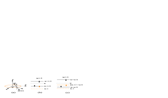
Figure 1: (Color online) (a) Schematic illustration of the spin orientation exhibited by the eigenstates of an ideal one-dimension ring. (b) and (c) show schematically the energy spectrums for the total angular momentum quantum number $\kappa$ at different spin-orbit coupling strengths $w=\cos^{-1}\gamma$.

The local spin orientations is inferred from the relations

$$S(\mathbf{r})_{\uparrow}=\frac{\hbar}{2}(\sin\gamma\cos\varphi\hat{e}_{x}+\sin\gamma\sin\varphi\hat{e}_{y}+\cos\gamma\hat{e}_{z}),$$ (11)

and

$$S(\mathbf{r})_{\downarrow}=\frac{\hbar}{2}[\sin(\pi-\gamma)\cos(\pi+\varphi)\hat{e}_{x}+\sin(\pi-\gamma)\sin(\pi+\varphi)\hat{e}_{y}+\cos(\pi-\gamma)\hat{e}_{z}].$$ (12)

Thus $\gamma$ is the angle illustrated in Fig. 1(a). The limit $Q_{R}\rightarrow\infty$, i.e. for a very strong SOI coupling, $\gamma\rightarrow-\pi/2$ which corresponds to the plane of the ring. The eigenenergies have the following structure

$$E_{n}^{S} = \frac{\hbar\omega_{0}}{2}\left[(n-x_{S})^{2}-\frac{Q_{R}^{2}}{4}\right],$$ (13)

$$x_{S} = \frac{\phi}{\phi_{0}}-\frac{1-Sw}{2}$$ (14)

where $w=\sqrt{1+Q_{R}^{2}}=1/\cos\gamma$, and $S=\pm 1$ stand for up and down spins. We emphasize that hereafter, the terms up and down (labeled respectively $\uparrow$ and $\downarrow$) refer to directions in the local frame, as illustrated in Fig. 1.

III.1.1 The weak SOI limit

In the weak SOI limit, i.e. if ($\gamma\to 0$) and in absence of the static external flux the eigenenergies attain the forms $E_{n}^{\uparrow}=\frac{\hbar\omega_{0}}{2}n^{2}$ and $E_{n}^{\downarrow}=\frac{\hbar\omega_{0}}{2}(n+1)^{2}$ which seems inconsistent with the spin-degenerate ground-state formula $E_{n}=\frac{\hbar\omega_{0}}{2}n^{2}$ (associated with $\hat{H}_{0}=\frac{\hbar^{2}}{2m^{*}a^{2}}(i\partial_{\varphi})^{2}$). The resolution of this apparent inconsistency is as follows. $H_{\text{SOI}}$ commutes in a nontrivial way with $K=L_{z}+S_{z}$ which is the z component of the total angular momentum, and with $S_{\gamma\varphi}=S_{x}\sin\gamma\cos\varphi+S_{y}\sin\gamma\sin\varphi+S_{z}\cos\gamma$ which is the spin component in the direction determined by the angles $\gamma$ and $\varphi$. Also we can show that $[K,S_{\gamma\varphi}]=0$. The simultaneous eigenfunctions of $H$, $K$ and $S_{\gamma\varphi}$ are the function given by Eq. (8). To rotate the quantization axis of $S_{z}$ to the direction $S_{\gamma\varphi}$, a SU(2) transformation is necessary, i.e. $US_{z}U^{-1}=S_{\gamma\varphi}$, where $U$ is the transformation matrix, $U_{11}=\cos\gamma/2\exp(-i\varphi/2)$, $U_{12}=-\sin\gamma/2\exp(-i\varphi/2)$, $U_{21}=\sin\gamma/2\exp(i\varphi/2)$, and $U_{22}=\cos\gamma/2\exp(i\varphi/2)$. Under the transformation of $U^{-1}$ the wave functions of SOI become $\Psi^{\prime}=U^{-1}\Psi_{n}^{S}(\varphi)=e^{i(n+1/2)\varphi}\chi_{S}$, where $\chi_{S}=(1,0)^{T}$ stands for spin-up state and $(0,1)^{T}$ for spin-down state. The exponential factor $n+1/2$ is the quantum number for the $z$ component of the total angular momentum, referred to as $K\Psi_{n}^{S}(\varphi)=\kappa\Psi_{n}^{S}(\varphi)$, where $\kappa=n+1/2$. $\kappa$ is fixed in the process of the SU(2) rotation. On the other hand, the wave function for $H_{0}$, the Hamiltonian for a ring without SOI, is usually set as $\Psi_{0}=e^{in\varphi}\chi_{S}$.matos1 Comparing $\Psi^{\prime}$ and $\Psi_{0}$, it is clear that the exponential factors in $\Psi^{\prime}$ and $\Psi_{0}$ are different, and $n$ in $\Psi_{0}$ is the quantum number of orbital momentum. This difference manifests itself in the limit $\gamma=0$ (i.e. SOI is zero, $H_{\text{SOI}}\to H_{0}$): the wavefunctions $\Psi_{n}^{S}(\varphi)$ do not go over in $\Psi_{0}$ because they are the eigenfunctions for different sets of commuting observables. The simultaneous set for $\Psi_{0}$ is $H$, $L_{z}$ and $S_{z}$.

Despite this explanation we may still wonder what is the physical effect of splitting of the energies on $n$ axis rashbajpc in the limit of vanishing SOI. We inspect therefore the persistent charge current (CC) caused by SOI and take the limit of absence of SOI in the last step. The partial charge persistent current due to the state labeled by $n$ and $S$ in the presence of SOI and a static external magnetic flux is

$$\mathbf{I}_{nS}=-\hat{\mathbf{e}}_{\varphi}I_{0}\left(n+\frac{\phi}{\phi_{0}}+\frac{1-Sw}{2}\right),$$ (15)

where $I_{0}=2E_{0}a/\phi_{0}$ is the unit of current. When $\phi=0$, the CC due to the particle in the $n$ level is $I_{nS}=-n$ for spin up and $I_{nS}=-(n+1)$ in the limit of zero SOI (we ignored $\hat{\mathbf{e}}_{\varphi}$ and scaled the current by $I_{0}$). The total CC is $I_{S}=\sum_{n}I_{nS}$. For a distribution of up spins, the occupied states are $n=0,\pm 1,\pm 2,\cdots$; for spin-down particles, they are $n=-1,(0,-2),(1,-3),\cdots$; the numbers in the same parenthesis “(…)” indicate states with the same energy. Hence, as expected, we conclude that the total CCs for up and down spins carriers are zero in the limit of vanishing external magnetic field and SOI. Note, that the lowest occupied state for down spin is not at $n=0$, but at $n=-1$. This means the velocity of the particle with down spin at $n=-1$ is zero; in fact $n+1$ stands for the quantized velocity for spin-down particles. Thus, shifting the energy spectrum in the down spin channel to the right by 1 quantum number, the energy spectrums for different spins become the same on the velocity axis which is consistent with the physical picture rashbajpc .

In presence of SOI the energy spectrum is rewritable as

$$E_{n}^{S}=\frac{\hbar\omega_{0}}{2}[(\kappa-Sw/2-\phi/\phi_{0})^{2}-Q_{R}^{2}/4]=\frac{\hbar\omega_{0}}{2}[(\kappa-\frac{1}{2}-x_{S})^{2}-Q_{R}^{2}/4].$$ (16)

For $\phi=0$ the energies associated with a total angular momentum quantum number $\kappa$ are spin-split; up spins have lower energy than down spins as illustrated in Fig. 1(b) and 1(c). For the case of zero SOI, i.e. for $w=1$ (cf. Fig. 1(b)) electrons with spin-up and $\kappa$ are degenerate with electrons having spin-down and $\kappa-1$ quantum numbers; the energy is given by $\kappa-1/2$, meaning that the energy levels are spin-degenerate.

III.2 Time-dependent wave functions and energies after pulse irradiation

As have been shown in detail matos1 ; matos2 ; mizushima ; berakdar , upon applying at $t=0$ a half-cycle pulse with a duration $\tau_{d}$, the time-dependent electronic states of the ring develop as

$$\Psi_{n}^{S}(\varphi,t_{0}=\tau_{d})=\Psi_{n}^{S}(\varphi,t=0)e^{i\alpha\cos\varphi}.$$ (17)

The parameter

$$\alpha=e\,a\,p/\hbar,\;p=-\int_{0}^{\tau_{d}}E(t)\rm{d}t$$ (18)

is the action (in units of action) taken over by the carriers from the pulse EM field. The range of validity of the the solution (17) has been discussed in Refs. [matos1, ; matos2, ; berakdar, ] (for a general discussion of the properties of the time development operator we refer to the work [mizushima, ]). The coherent state (17) is not an eigenstate of the ring for $t>t_{0}$, in fact a state initially labeled by the quantum numbers $n_{0}$ and $S_{0}$ is expressible in terms of the ring stationary eigenstates as

$$\Psi_{n_{0}}^{S_{0}}(\varphi,t)=\frac{1}{\sqrt{2\pi}}\sum_{ns}C_{n}^{S}(n_{0},S_{0},t)e^{i(n+1/2)\varphi}e^{-iE_{n}^{S}t/\hbar}|\nu^{S}\rangle,$$ (19)

where $|\nu^{S}\rangle=\nu^{S}(\gamma,\varphi)$. From Eq. (17) we deduce the expansion coefficients

$$C_{n}^{S}=\left\{\begin{array}[]{l l}\delta_{SS_{0}}\delta_{nn_{0}},&\text{for t}\leq 0,\\ \delta_{SS_{0}}i^{n_{0}-n}J_{n_{0}-n}(\alpha),&\text{for t}>t_{0},\end{array}\right.$$ (20)

The energy at time $t$ is then given by the relations

$$E_{n_{0}}^{S_{0}}(t) = \langle\Psi_{n_{0}}^{S_{0}}(\varphi,t)|H|\Psi_{n_{0}}^{S_{0}}(\varphi,t)\rangle=i\hbar\langle\Psi_{n_{0}}^{S_{0}}(\varphi,t)|\frac{\partial}{\partial t}|\Psi_{n_{0}}^{S_{0}}(\varphi,t)\rangle$$ (21)

$$= \sum_{ns}E_{n}^{S}|C_{n}^{S}(n_{0},S_{0},t)|^{2}.$$

Substituting Eq. (13) in Eq. (21) we find

$$E_{n_{0}}^{S_{0}}(t) = \frac{\hbar\omega_{0}}{2}\left\{(n_{0}-x_{S_{0}})^{2}+\frac{2\alpha^{2}\;\Theta(t-t_{0})-Q_{R}^{2}}{4}\right\};$$ (22)

$$E_{n_{0}}^{S_{0}}(t>t_{0}) = E_{n_{0}}^{S_{0}}(t<0)+\frac{\hbar\omega_{0}}{2}\frac{\alpha^{2}}{2}.$$ (23)

Here $\Theta(t)$ is the Heaviside step function and $x_{S}$ is given by Eq. (14).

IV Dipole moment generated by the pulse under external static magnetic field

Having identified the time-dependent spectrum and eigenfunctions, we focus now on the charge-dynamics and the induced polarization. To this end we inspect the charge localization parameter, defined as matos1 ; matos2 ; moskalenko

$$\langle\cos\varphi\rangle_{n_{0}}^{S_{0}}(t) = \int_{0}^{2\pi}d\varphi|\Psi_{n_{0}}^{S_{0}}(\varphi,t)|^{2}\cos\varphi,$$ (24)

$$= \frac{1}{2}\sum_{ns}\left\{C_{n}^{S*}C_{n-1}^{S}e^{i(E_{n}^{S}-E_{n-1}^{S})t/\hbar}+C_{n}^{S*}C_{n+1}^{S}e^{i(E_{n}^{S}-E_{n+1}^{S})t/\hbar}\right\}.$$

From Eq. (13) and relation (20) for the coefficients, the localization parameter is deduced after some algebra to be

$$\langle\cos\varphi\rangle_{n_{0}}^{S_{0}}(t)=\alpha\,h(\Omega)\,\sin(b)\,\cos[2(n_{0}-x_{S_{0}})b],$$ (25)

$$h(\Omega)=J_{0}(\Omega)+J_{2}(\Omega),\,b=\omega_{0}t/2,\mbox{ and }\Omega=\alpha\sqrt{2(1-\cos(2b))}.$$

Here $J_{n}$ is a Bessel function with index $n$. The partial photo-induced dipole moment $\mu_{n_{0}}^{S_{0}}(t)$ associated with the initial state with quantum numbers $n_{0}$, $S_{0}$ and the total HCP-induced dipole moment along the $x$ axis $\mu^{S_{0}}(t)$ for the initial spin $S_{0}$ read

$$\mu_{n_{0}}^{S_{0}}(t) = ea\langle\cos\varphi\rangle_{n_{0}}^{S_{0}}(t),$$ (26)

$$\mu^{S_{0}}(t) = \sum_{E_{n_{0}}^{S_{0}}\leq E_{F}}f(n_{0},S_{0},N,t)\mu_{n_{0}}^{S_{0}}(t).$$ (27)

$f$ stands for the nonequilibrium distribution function whose derivation requires the solution of the kinetic equations. In principle we can employ our recent approach based on the density matrix andrey06 but more detailed knowledge on the spin-dependent decay channels in confined geometry is needed. Here we inspect the zero temperature behaviour of the induced dipole moment and the associated emission spectrum. We expect the qualitative features of these physical quantities to persist at finite temperatures, as we demonstrated for the case of vanishing SOI andrey06 .

IV.1 Spectral analysis

In the following we focus on the spectral properties. The spin-orbit interaction breaks the energy-degeneracy of $n$ and $-n$ states. As evident from Eqs. (14,22) the spectrum, posses a symmetry axis (SA) located at $x_{S}=\phi/\phi_{0}-(1-Sw)/2$ (the global additional pulse-associated energy and SOI-induced energy shift do not affect this symmetry), i.e. the static magnetic flux and the SOI act as an effective magnetic field. In Eq. (22) $n_{0}$ is an integer, hence it is advantageous to introduce the integer parameter $l_{S}$ as the nearest integer that is less than $x_{S}$ and define ($\sigma=\uparrow$ or $\downarrow$)

$$\Delta_{\sigma}=x_{S}-l_{S}$$ (28)

whose meaning is illustrated in Fig. 2(c) and 2(d). We distinguish four cases (a), (b), (c) and (d) corresponding to $\Delta_{\sigma}=0,1/2$, $\Delta_{\sigma}\in\,[0,1/2]$ and $\Delta_{\sigma}\in\,[1/2,1]$, respectively (cf. Fig. 2). $\Delta_{\sigma}=1$ is equivalent to $\Delta_{\sigma}=0$, thus $\Delta_{\sigma}$ is periodic with changing SA and varies within the fundamental interval $[0,1]$. Furthermore, we introduce

$$\bar{\Delta}_{\sigma}=|1/2-\Delta_{\sigma}|,$$ (29)

as the distance between the SA and the half integer axis. These four cases in Fig. 2 are valid for up and spin-down states.

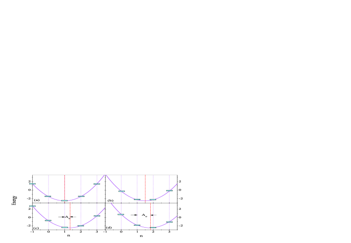
Figure 2: (Color online) (a) SA has an integer value; (b) SA is a half integer; (c) SA lies in the region $(l,l+1/2)$; (d) SA is in the region $(l+1/2,l+1)$. The red dash lines are the SA in each case.

IV.1.1 Spinless particles

The two spin states, up and down, need to be considered. Allowing each of these two spins to occupy the four configurations shown in Fig. 2, results in 16 combinations. For simplicity, we consider at first only one kind of spins and states which can be any of the four cases depicted in Fig. 2. Depending on the total number of electrons in the ring $N$ two situations are distinguished:

(1) $N$ is an even integer. For case (a) in Fig. 2 (for brevity we refer hereafter to cases (a), (b), $\cdots$; and write $l_{S}\equiv l$, $\Delta_{\sigma}\equiv\Delta$, and $x_{S}\equiv x$) the occupied states are at $n_{0}=\frac{1}{2}(l-m),l-(m-1),\cdots,l-1,l,l+1,l+2,\cdots,l+(m-1),\frac{1}{2}(l+m)$. Here, e.g. $\frac{1}{2}(l-m)$ means half occupation on the state characterized by the quantum number $l-m$. The dipole moment in this case $\mu_{(a)}^{e}(N,t)$ reads

$$\mu_{(a)}^{e}(N,t) = \alpha\Theta(t-t_{0})h(\Omega)\sin b\sum_{n_{0}}\cos[2(n_{0}-x)b],$$ (30)

$$= \alpha\Theta(t-t_{0})h(\Omega)\,\sin(Nb)\,\cos(b).$$

For (b), (c) and (d) cases, we have $n_{0}=l-(m-1),\cdots,l-1,l,l+1,l+2,\cdots,l+(m-1),l+m$. Accordingly we deduce

$$\mu_{(bcd)}^{e}(N,t)=\alpha\Theta(t-t_{0})h(\Omega)\,\sin(Nb)\,\cos[(1-2\Delta)b],$$ (31)

where $\Delta=x-l$. In (a) case, $\Delta=0$, then Eq. (31) will reduce to Eq. (30). The dipole moment for even occupation has in general the form

$$\mu^{e}(N,\Delta,t)=\alpha\Theta(t-t_{0})h(\Omega)\,\sin(Nb)\,\cos[(1-2\Delta)b].$$ (32)

(2) $N$ is an odd integer. Similar steps as in the proceeding case can be performed, leading us to conclude that

$$\mu^{o}(N,\bar{\Delta},t)=\alpha\Theta(t-t_{0})h(\Omega)\sin(Nb)\,\cos[(1-2\bar{\Delta})b].$$ (33)

IV.1.2 Spin-$\frac{1}{2}$ particles and $\phi\neq 0$

For spin-$\frac{1}{2}$ particles the energy spectrum is spin-dependent. The position of the spectrum SA is different for the two spin states, i.e. $x_{\uparrow}=\phi/\phi_{0}+(w-1)/2$ and $x_{\downarrow}=x_{\uparrow}-w$. Thus, the relative distance between these two SAs depends on the external flux and SOI parameter $w$. Scanning these parameters the spectrums of up and down spins are tuned to any of the four cases shown in Fig. 2. In what follows we use for cases in Fig. 2 that correspond to the spin-down and the spin-up states the symbols (ij) (i,j=a,b,c,d); e.g. the case (ab) means the down-spin spectrum corresponds to the case (a) whereas the up-spin spectrum is as in case (b); hence there are 16 combinations of such pairs to be considered. In the following, we consider four different occupations in the ring for up and spin-down states and these 16 combinations in detail.

(1) Even number of pairs. For $N=4m$, where $m$ is an integer ($N$ is the total number of electrons in the ring) there are $2m$ spin-up particles and $2m$ spin-down particles occupying the respective spectrums, meaning that

$$\mu^{\sigma}(N,t)=\mu^{e}(N/2,\Delta_{\sigma},t).$$ (34)

(2) Odd number of pairs. If $N=4m+2$ then $2m+1$ spin-up particles and $2m+1$ spin-down particles populate the respective spectrums and

$$\mu^{\sigma}(N,t)=\mu^{o}(N/2,\bar{\Delta}_{\sigma},t).$$ (35)

(3) Even number of pairs plus an extra particle. Here we write $N=4m+1$. i) For $2m$ spin-up particles and $2m+1$ spin-down particles we find $\mu^{\uparrow}(2m,t)=\mu^{e}(2m,\Delta_{\uparrow},t)$, and $\mu^{\downarrow}(2m+1,t)=\mu^{o}(2m+1,\bar{\Delta}_{\downarrow},t)$. Cases (ab), (ac), (ad), (cb), (db) belong to this type. ii) If there are $2m+1$ spin-up particles and $2m$ spin-down particles in the ring we infer $\mu^{\uparrow}(2m+1,t)=\mu^{o}(2m+1,\bar{\Delta}_{\uparrow},t)$, and $\mu^{\downarrow}(2m,t)=\mu^{e}(2m,\Delta_{\downarrow},t)$. Cases (ba), (ca), (da), (bc), (bd) belong to this category. iii) If we have $2m$ spin-up particles and $2m$ spin-down particles plus one extra particle we shall analyze the populated state of the extra particle. E.g., cases (aa), (bb), (cc), (dd), (cd) and (dc)are possible situations. Careful calculation of all cases results in the formula

$$\mu_{ex}=\alpha\Theta(t-t_{0})h(\Omega)\sin(b)\cos[(2m+1-2\bar{\Delta}_{\sigma})b],$$ (36)

where $\bar{\Delta}_{\sigma}\geq\bar{\Delta}_{\bar{\sigma}}$.

(4) Odd number of pairs plus an extra particle. For $N=4m+3$ we distinguish: i) For $2m+1$ spin-up particles and $2m+2$ spin-down particles we infer $\mu^{\uparrow}(2m+1,t)=\mu^{o}(2m+1,\bar{\Delta}_{\uparrow},t)$, and $\mu^{\downarrow}(2m+2,t)=\mu^{e}(2m+2,\Delta_{\downarrow},t)$. Cases (ab), (ac), (ad), (cb) and (db) belong to this type. ii) For $2m+2$ spin-up and $2m+1$ spin-down particles we deduce $\mu^{\uparrow}(2m+2,t)=\mu^{e}(2m+2,\Delta_{\uparrow},t)$, and $\mu^{\downarrow}(2m+1,t)=\mu^{o}(2m+1,\bar{\Delta}_{\downarrow},t)$. Cases (ba), (bc), (bd), (ca) and (da) are examples for this situation. iii) For $2m+1$ spin-up and for $2m+1$ spin-down particles plus an extra particle (cf. (bb), (cc), (dd), (cd) and (dc)) we find for the dipole moment

$$\mu_{ex}=\alpha\Theta(t-t_{0})h(\Omega)\sin(b)\cos[(2m+1+2\bar{\Delta}_{\sigma})b]$$ (37)

where $\bar{\Delta}_{\sigma}\leq\bar{\Delta}_{\bar{\sigma}}$.

IV.1.3 spin $\frac{1}{2}$ particles with ($\phi=0$)

If $\phi=0$ then $x_{\uparrow}=\frac{w-1}{2}$, $x_{\downarrow}=-\frac{1+w}{2}$, and $\Delta_{\uparrow}+\Delta_{\downarrow}=1$ applies. The symmetry axes for up and down-spin states have the same distance from the nearest integer axes to the left and to the right sides to the SAs. The dipole moments are spin degenerate.

(1) Even number of pairs and $\phi=0$. For $N=4m$ we find $\mu^{\uparrow}(N,t)$=$\mu_{\uparrow}^{e}(2m,\Delta_{\uparrow},t)$.
(2) Odd number of pairs and $\phi=0$. For $N=4m+2$ we conclude $\mu^{\uparrow}(N,t)$=$\mu_{\uparrow}^{o}(2m+1,\bar{\Delta}_{\uparrow},t)$.
(3) Even number of pairs plus an extra particle. If $N=4m+1$, only possible combinations are (aa), (bb), (cd) and (dc). The spin degeneracy of the extra particle is caused by the crossing of the energy levels with opposite spins. The dipole moment reads

$$\mu^{\uparrow}(N,t)=\frac{1}{2}\alpha\Theta(t-t_{0})h(\Omega)\left\{\sin(2mb)\cos[(1-2\Delta_{\uparrow})b]+\sin[(2m+1)b]\cos(2\Delta_{\uparrow}b)\right\}.$$ (38)

If $\Delta_{\uparrow}=0$, Eq. (38) delivers the dipole moment for the case (aa) whereas $\Delta_{\uparrow}=1/2$ applies for the case (bb) and others for case (cd) and (dc).
(4) Odd number of pairs plus an extra particle. For $N=4m+3$, only (aa), (bb), (cd) and (dc) are applicable. The dipole moment is

$$\mu^{\uparrow}(N,t)=\frac{1}{2}\alpha\Theta(t-t_{0})h(\Omega)\left\{\sin[(2m+1)b]\cos[(1-2\bar{\Delta}_{\uparrow})b]+\sin[(2m+2)b]\cos(2\bar{\Delta}_{\uparrow}b)\right\}.$$ (39)

In the event $\bar{\Delta}_{\uparrow}=0$, Eq. (39) yields the dipole moment for case (bb) whereas $\bar{\Delta}_{\uparrow}=1/2$ is valid for the case (aa) and others for case (cd) and (dc).

V Numerical Results and Discussions

V.1 Experimental feasibility and general remarks

In this section we present and analyze numerical results for the HCP-induced polarization of a ballistic quantum ring. In view of an experimental realization it is important to identify the realistic range of the parameters such as the strength of the SOI and the associated quantities. The range of the ring size and external field strength are chosen according to current experimental feasibility.

The Rashba SOI was already investigated for numerous semiconductor quantum wells such as In_xGa_1-xAs/InP quantum wells thsch , In_0.53Ga_0.47As/In_0.52Ga_0.48As heterostructures ingaas , and GaSb/InAs/GaSb quantum wells luo . Spin-interference effects in a ring with Rashba SOI which was built in a InGaAs/InAlAs heterostructure was the subject of Ref. [nitta03, ], and the Aharonov-Casher phase was inspected in II-VI semiconductor quantum rings, such as HgTe/HgCdTe ring konig . In the context of the present work it is important to estimate the realistic range for the spin orbit angle $\gamma$ for the relevant semiconductor materials: For In_xGa_1-xAs/InP quantum well thsch , $\alpha_{R}$ varies in the range $[0.7\times 10^{-11}eV\cdot m,1.1\times 10^{-11}eV\cdot m]$ when an applied gate voltage varies from +1.5 V to -2.5 V; this corresponds to $\gamma$ being in the range $[-34^{\circ},-47^{\circ}]$, $[-74^{\circ},-79^{\circ}]$, and $[-82^{\circ},-85^{\circ}]$ for rings with 100 nm, 500 nm, and 1 $\mu m$ radius respectively ($m^{*}=0.037m_{0}$, $m_{0}$ is the free carrier mass). For In_0.53Ga_0.47As/In_0.52Ga_0.48As materials ingaas , $\alpha_{R}$ varies in $[0.5\times 10^{-11}eV\cdot m,1.0\times 10^{-11}eV\cdot m]$ if the external gate voltage changes from +1.5 V to -1 V; correspondingly $\gamma$ varies in $[-33^{\circ},-52^{\circ}]$, $[-73^{\circ},-81^{\circ}]$, and $[-81^{\circ},-86^{\circ}]$ for rings with 100 nm, 500 nm, and 1 $\mu m$ radius respectively ($m^{*}=0.05m_{0}$). For GaSb/InAs/GaSb quantum well luo the values of $\gamma$ are on the same order as above.

With regard to available pulses, a wide range of pulse durations and strengths have been realized hcp ; seqhcp1 ; seqhcp2 ; seqhcp3 ; seqhcp4 . As clear from the above analysis the pulse parameter which is decisive for the electron dynamics is $\alpha$ as given by Eq. (18). For pulse with a sin-square shape and a duration of $\tau_{d}=1$ ps we achieve for a ring with radius $1~{}\mu$m a transferred action of $\alpha_{1}=0.1$, $\alpha_{2}=1$, and $\alpha_{3}=10$ if the peak electric field strength is tuned to respectively $E_{1}=1.32~{}$V/cm, $E_{2}=13.2~{}$V/cm, and $E_{3}=132~{}$V/cm. It is this range of $\alpha$ which we use in the present numerical calculations. In the figures below we just provide $\alpha$.

From a general point of view we can expect four frequency scales to be relevant for the time-dependent charge and spin dynamics:
1). The global energy scale is set by the size of the system. Hence, the fundamental frequency is given by $\omega_{0}=\hbar/(m^{*}a^{2})$ and the natural time scale is $t_{p}=4\pi/\omega_{0}$ which for the ring sizes at hand is tens of picoseconds.
2). As for any fermionic system, the Fermi energy $E_{F}$ sets the scale for the fast (femtosecond) charge dynamics associated with excitation near $E_{F}$. Since we are dealing with an isolated ring the Fermi energy is expressible in terms of the number of particles $N$ and the relevant frequency is therefore $N\omega_{0}$.
3). A Further frequency $\omega_{R}$ is associated with SOI-influenced dynamics; $\omega_{R}=2\alpha_{R}/(\hbar a)$. For our systems $\omega_{R}$ can be on the order of $\omega_{0}$ opening the possibility for controlling quantum interferences, e.g. by tuning the strength of SOI (via a gate voltage).
4). Further modifications are brought about by the applied pulse which (for the pulses of interest here) induces a multitude of excitations near $E_{F}$ with further associated frequencies, as detailed below.

These physical expectations are confirmed by the general structure of the calculations for the induced dipole moments according to Eqs. (25,30,32,33,36,37)

V.2 Zero static magnetic field

At first we investigate the case of vanishing static flux ($\phi=0$). In Fig. 3 the time-dependence of the dipole moment is shown for different spin-orbit angles $\gamma$ and pulse strengths $\alpha$. Because of the spin-degeneracy we consider only one spin channel. The total number of particles is $N=4m$. The time is measured in units of the system’s time scale $t_{p}=4\pi m^{*}a^{2}/\hbar$.

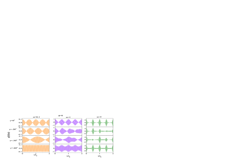
Figure 3: (color online) The time-dependence (in units of $t_{p}=4\pi/\omega_{0}$) of the net pulse-induced dipole moment $\mu(t)$ (in units of $ea$) in the up or down-spin channel at different $\gamma$ and $\alpha$ as depicted on the figure. The total number of particles is $N=100$ and $\phi=0$.

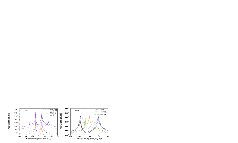
Figure 4: (color online) The emission spectrum for different pulse strengths (quantified by $\alpha$) and SOI strengths (indicated by $\gamma$). In (a) $\alpha$ is varied at $\gamma=0$ whereas in (b) $\gamma$ is variable at fixed $\alpha=0.01$; in both cases $N=100$.

The four time scales mentioned above are clearly visible. As inferred from Eqs. (30, 32, 33, 36, 37) the net time-dependent dipole moment grows linearly with the pulse field strength at small $\alpha$ (note for $\alpha\ll 1/2$, $\Omega\ll 1$, we have $h(\Omega)\approx 1$). The fast oscillation in the dipole moment are related the transition between the levels near $E_{F}$ (Rabi flopping). With increasing $\alpha$ more levels are excited giving rise to higher contributing harmonics (cf. $\alpha=1$ and $\alpha=3$ in Fig. 3 and also Fig. 4).

The SOI strength (quantified by $\gamma$) has a dramatic influence on the low frequency modulation of the dipole-moment envelope. The low frequency is associated with the difference between the frequencies of the involved levels near $E_{F}$, which is on the scale of $\omega_{0}$. In fact, as inferred from Eq. (32) $\gamma$ can be tuned as to influence the phases of the involved wave functions changing thus the interference pattern and removing eventually the slow oscillations altogether. This happens at $\gamma=-60^{\circ}$ as shown in Fig. 3. When $|\gamma|$ is increased further the slow modes appear again. This is insofar important as $\gamma$ can be modified by an external gate voltage offering thus the possibility of engineering the emission spectrum via an applied static electric field and opening the way for testing experimentally our theoretical predictions. For this reason we inspect the power spectrum alex_power produced by the non-equilibrium charge oscillations in the QR by evaluating

$$P(\omega)=|\mu(\omega)|^{2},\quad\mu(\omega)=\int_{-\infty}^{\infty}\mu(t)e^{-i\omega t}dt.$$ (40)

Fig. 4 shows the power spectrum for different strengths of the pulse $\alpha$. As evident from these calculations the frequency scale is set by $\omega_{0}/2$. In Fig. 4 the number of particles occupying the single spin states is N=50, for small $\alpha$ only the state at $E_{F}$ is excited leading to the appearance of two frequencies at $(N-1)\omega_{0}/2$ and $(N+1)\omega_{0}/2$. With increasing $\alpha$, more levels are excited and correspondingly further frequencies in unit of $\omega_{0}/2$ emerge at $47,45,\cdots$ and $53,55,57,\cdots$ (see Fig. 4(a)). In this context we note that a very short HCP contains almost all frequencies. Nevertheless, at low intensities only a limited number of states in the ring can be excited. The reason is obvious from Eq. (23). The highest energy level achieved upon excitation is $E_{F}+\hbar\omega_{0}\alpha^{2}/4$. Hence there is an excited energy cut-off set by the field intensity (available photons) and limits consequently for a certain $\alpha$ the number of possible frequencies observable in the power spectrum (as seen in Fig. 4).

Fig. 4(b) shows how the SOI shifts of the frequencies: with increasing $|\gamma|$ the frequency at 49 moves towards a higher frequency while the frequency at 51 moves to a lower frequency. For the angle $\gamma=-60^{\circ}$ we infer $\Delta=1/2$ and the two frequencies merge into one frequency. Further increasing the SOI strength, i.e. $\Delta>1/2$, the frequency peak from 51 continues moving to 49, while the frequency peak from 49 approaches 51 until they coincide for $\Delta=1$ (or $\Delta=0$). This behavior of frequencies is repeated periodically with increasing SOI.

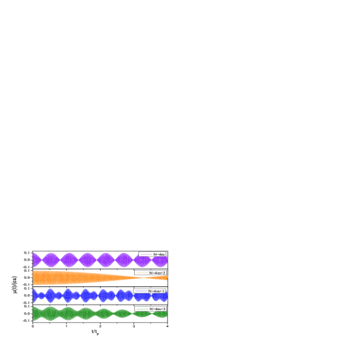
Figure 5: (color online) The time-dependence of dipole moment is shown at different occupation numbers. Here $\gamma=-70^{\circ}$, $\alpha=0.1$ and $m=25$. Units are as in Fig. 3.

As detailed above the dipole moment depends sensitively on the occupation numbers. Fig. 5 shows an example of the dipole-moment dynamics for $N=4m+2$ contrasted with the case $N=4m$. We remark that since $\Delta+\bar{\Delta}=1/2$ we have $\Delta=0(\frac{1}{2})$ for $\bar{\Delta}=\frac{1}{2}(0)$. Thus for $N=4m$, when the dipole moment increases with $\Delta$ in $\Delta\in[0,\frac{1}{2}]$ the dipole moment decreases for the case $N=4m+2$. Furthermore, the parity of the occupation number is very important for the property of dipole moment of the ring. E.g., for $\Delta\approx\bar{\Delta}$, the case $N=4m$ ($N=4m+1$) behaves similarly to $N=4m+2$ ($N=4m+3$) in which cases the occupations are even (odd). However, the even case is qualitatively different from the odd case (not shown in Fig. 5). If $\Delta\neq\bar{\Delta}$ the oscillations of the dipole moment are different in all the cases depicted in Fig. 5.

V.3 Finite static magnetic field

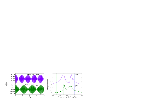
Figure 6: (color online) The time-dependence of the dipole moment for up and down spins under a nonzero static magnetic field are shown in (a) and (b). The power spectra corresponding to the up and down spins are shown in (c) and (d) respectively. Here $\phi=0.25$, $\gamma=-70^{\circ}$, $\alpha=0.1$ and $N=100$.

A static external magnetic field lifts the spin degeneracy of the dipole moment. The induced dipole moment dynamics becomes spin dependent (cf. Fig. 6). The slow-frequency shift between the dipole-moment oscillations in the up-spin and down-spin channels is readily understood from the energy splitting (cf. Eq. (23)). The power spectrums for the up and down-spins dipole oscillations (Fig. 6(c) and 6(d)) reveals clearly the frequency shift.

For more insight into the role of the SOI we investigate the spin-resolved local charge density before and after the pulse. The probability density associated with the level labeled by $n_{0}$ and $S_{0}$ is $\rho_{n_{0}}^{S_{0}}(\varphi,t)=|\Psi_{n_{0}}^{S_{0}}(\varphi,t)|^{2}$. Before the pulse the charge density is a unit charge uniformly distributed around the ring, i.e. $\rho_{0}=1/(2\pi)$. Upon applying the pulse we find

$$\rho_{n_{0}}^{S_{0}}(\varphi,t>0)=\rho_{0}+\vartriangle\rho_{n_{0}}^{S_{0}}(\varphi,t>0),$$ (41)

where the second term is the spin-resolved, field-induced charge density variation (ICDV) which we evaluated and find

$$\vartriangle\rho_{n_{0}}^{S_{0}}(\varphi,t>0) = \frac{1}{\pi}\{\sum_{n=0}^{\infty}J_{2n+1}[2\alpha\sin(2n+1)b]\cos(2n+1)[\varphi-2(n_{0}-x_{S_{0}})b]$$ (42)

$$+\sum_{n=1}^{\infty}J_{2n}[2\alpha\sin(2nb)]\cos 2n[\varphi-2(n_{0}-x_{S_{0}})b]\}.$$

The total spin-resolved charge density is obtained from a sum over the occupied levels $\rho^{S_{0}}(\varphi,t>0)=N_{S_{0}}\rho_{0}+\vartriangle\rho^{S_{0}}(\varphi,t>0),$ where $N_{S_{0}}$ is the total particle number in the $S_{0}$ spin channel. The term $\vartriangle\rho^{S_{0}}(\varphi,t>0)$ for the even pair occupation case is

$$\vartriangle\rho^{S_{0}}(\varphi,t>0) = \frac{\alpha}{\pi}\{\sum_{n=0}^{\infty}\frac{1}{2n+1}[J_{2n}(\Omega_{1n})+J_{2n+2}(\Omega_{1n})]\sin[N_{S_{0}}(2n+1)b]\cos(2n+1)\varphi_{S_{0}}(t)$$ (43)

$$+\sum_{n=1}^{\infty}\frac{1}{2n}[J_{2n-1}(\Omega_{2n})+J_{2n+1}(\Omega_{2n})]\sin(N_{S_{0}}2nb)\cos 2n\varphi_{S_{0}}(t)\},$$

where $\Omega_{1n}=a\alpha\sin(2n+1)b$, $\Omega_{2n}=a\alpha\sin(2nb)$, and $\varphi_{S_{0}}(t)=\varphi-(1-2\Delta_{S_{0}})b$.

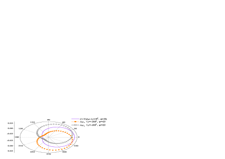
Figure 7: (color online) A snap-shot of the pulse-induced charge density variation (ICDV) as a function of the azimuthal angle $\varphi$ at the time $t/t_{p}=2.005$. The pulse parameter is $\alpha=0.1$, and $N=100$. Full (open) dots show the ICDV in the up (down) spin channel. Solid curve stands for the spin-averaged ICDV.

Eq. (43) indicates a spin-dependent phase of $\vartriangle\rho^{S_{0}}$ caused by the interplay of SOI, the static magnetic field, and the pulse field. Interestingly the phase shift evolves with time. Fig. 7 shows the time-evolution of the spin-dependent ICDV. In all cases depicted in Fig. 7 the static flux is absent. For $\gamma=0$ we observe, as expected, how the pulse kicks the charge density along the pulse-polarization axis. For the given time moment, the missing charge density around $\varphi=\pi$ is pushed to the region around $\varphi=0$. For a finite spin orbit interaction ($|\gamma|>0$) we observe a spin splitting of ICDV, meaning that the pulse induces temporally and locally a finite spin polarization $P=\rho_{\uparrow}-\rho_{\downarrow}$, even though the system is initially paramagnetic. The time integral of the pulse-induced, local spin polarization vanishes however. Technically, we infer that the SOI results in a SU(2) flux that produces opposite phase shifts on the azimuthal angle with the same magnitude for a zero-static magnetic field, i.e. $\varphi_{\uparrow(\downarrow)}=\varphi\mp(1-2\Delta_{\uparrow})b$. These shifts cause a rotation around the ring of the symmetry axes of the spin-up and the spin-down densities respectively clockwise and anticlockwise (see Fig. 7). When $\gamma=-60^{\circ}$ ($\Delta_{\uparrow}=1/2$), the up and down ICDV merge into one curve after one period. The periodic rotation is subject to the condition $\Delta_{\uparrow}=1/2$. The spin-averaged ICDV, i.e. $\vartriangle\rho=\vartriangle\rho_{\uparrow}+\vartriangle\rho_{\downarrow}$, is always symmetric with respect to $x$ axis. At $\varphi=0$ and $\pi$ ICDV is spin-degenerate for all times ($P(t)=0$).

The time evolution of the spin-resolved ICDV is depicted in Fig. 8. The symmetry axes of the pulse-induced spin-up and spin-down ICDV rotate around the ring respectively anticlockwise and clockwise with time (which is the opposite behaviour when increasing SOI). Accordingly the total ICDV oscillates along the $x$ axis and possesses a left-right symmetry with respect $x$. The local and temporal spin polarization $P$ is symmetric to $y$ axis and oscillates along it with the same frequency as $\rho_{\uparrow}$ (or $\rho_{\uparrow}$).

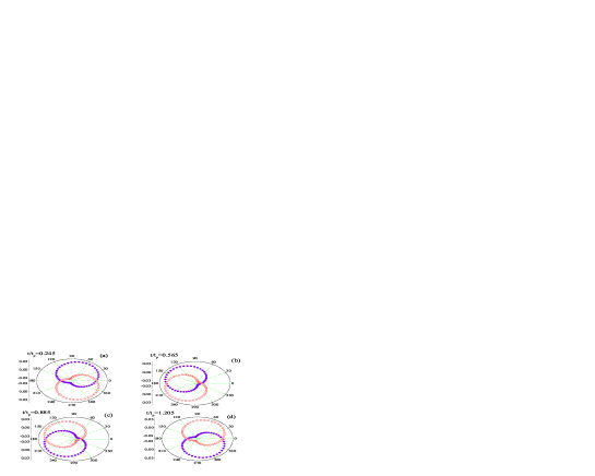
Figure 8: (color online) The time and spatial dependence of the ICDV shown in polar coordinates in (a), (b), (c) and (d) at different times after the pulse. Filled circles represent the up spin ICDV and the open circles indicate the down spin ICDV. The parameters are $\alpha=0.1$, $\phi=0$, $\gamma=-40^{\circ}$ and $N=100$.

VI Conclusios

In summary, we investigated the dynamical response of a quantum ring with spin-orbit interaction upon the application of a linearly polarized time-asymmetric weak electromagnetic pulse. It is found that the dipole moment along the pulse polarization axis is spin degenerate when there is no external magnetic field. The dipole moment oscillates with time and the SOI provides an envelope function or shifts of the oscillation frequencies of dipole moment. Stronger pulse fields can excite higher and lower harmonics. And the envelope functions for different parity of the occupation number on the ring are different. When a static external magnetic field is applied, the spin degeneracy is removed. The spatial and temporal dependence of the pulse induced charge-density variation (ICDV) indicates that the SOI results in a SU(2) flux leading to a splitting of the phases of the up and down spins states. The symmetric axes of the ICDV for the up and down spins are rotated equally in clockwise and anticlockwise when increasing SOI. The total ICDV and the local and temporal polarization of the charge density are symmetric to respectively the light polarization axis and the axis perpendicular. The pulse-induced polarization is experimentally accessible by measuring the power spectrum of the emitted radiation.

We thank A.S. Moskalenko and A. Matos-Abiague for fruitful discussions. The work is support by the cluster of excellence ”Nanostructured Materials” of the state Saxony-Anhalt.

References

- (1) T. Heinzel, Mesoscopic Electronics in Solid State Nanostructures (Wiley-VCH Verlag, Weinheim, 2003).
- (2) Y. Imry, Introduction to Mesoscopic Physics (Oxford University Press, Oxford, 2002).
- (3) L. W. Yu, et al., Phys. Rev. Lett. 98 166102 (2007); Advanced Materials 19, 1577 (2007);
- (4) D. Mailly, C. Chapelier, and A. Benoit, Phys. Rev. Lett. 70, 2020 (1993).
- (5) W. Rabaud, et al., Phys. Rev. Lett. 86, 3124 (2001).
- (6) A. Fuhrer et al., Nature 413, 822 (2001).
- (7) A. Lorke et al., Phys. Rev. Lett. 84, 2223 (2000).
- (8) J. Nitta, F. E. Meijer, and H. Takayanagi, Appl. Phys. Lett. 75, 695 (1999).
- (9) V. E. Kravtsov, and V. I. Yudson, Phys. Rev. Lett. 70, 210 (1993); O. L. Chalaev, and V. E. Kravtsov, ibid 89, 176601 (2002).
- (10) O. L. Chalaev, and V. E. Kravtsov, Phys. Rev. Lett. 89, 176601 (2002).
- (11) P. Kopietz, and A. Völker, Euro. Phys. J. B 3, 397 (1998).
- (12) M. Moskalets, and M. Büttiker, Phys. Rev. B 66, 245321 (2002).
- (13) L. I. Magarill, and A. V. Chaplik, JETP Lett. 70, 615 (1999).
- (14) V. Gudmundsson, C. -S. Tang, and A. Manolescu, Phys. Rev. B 67, 161301(R) (2003); S. S. Gylfadóttir, et. al., Physica Scripta T114, 41 (2004); Physica E 27, 278 (2005).
- (15) A. Matos-Abiague, and J. Berakdar, Eorophys. Lett. 69, 277 (2005).
- (16) A. Matos-Abiague, and J. Berakdar, Phys. Rev. Lett. 94, 166801 (2005).
- (17) A. Matos-Abiague, and J. Berakdar, Phys. Rev. B 70, 195338 (2004).
- (18) Y. V. Pershin, and C. Piermarocchi, Phys. Rev. B 72, 245331 (2005).
- (19) I. Barth, J. Manz, Y. Shigeta, and K. Yagi, J. Am. Chem. Soc. 128, 7043 (2006).
- (20) A. S. Moskalenko, A. Matos-Abiague, and J. Berakdar, Phys. Rev. B 74, 161303 (2006).
- (21) D. You, R. R. Jones, P. H. Bucksbaum and D. R. Dykaar, Opt. Lett. 18, 290 (1993).
- (22) T. J. Bensky, G. Haeffler, and R. R. Jones, Phys. Rev. Lett. 79, 2018 (1997).
- (23) A. Wetzels, A. Gürtel, H. G. Muller, and L. D. Noordam, Eur. Phys. J. D 14, 157 (2001).
- (24) M. T. Frey et al., Phys. Rev. A 59, 1434 (1999).
- (25) H. Maeda, J. Nunkaew, and T. E. Gallagher, Phys. Rev. A 75, 053417 (2007).
- (26) Y. Meir, Y. Gefen, O. Entin-Wohlman, Phys. Rev. Lett. 63, 798 (1989).
- (27) A. V. Chaplik, and L. I. Magarill, Superlattice and Microstructures, 18, 321 (1995).
- (28) J. Splettstoesser, M. Governale, and U. Zülicke, Phys. Rev. B 68, 165341 (2003).
- (29) D. Frustaglia, and K. Richter, Phys. Rev. B 69, 235310 (2004).
- (30) B. Molnár, F. M. Peeters, and P. Vasilopoulos, Phys. Rev. B 69, 155335 (2004); 72, 75330 (2005).
- (31) P. Földi, et al., Phys. Rev. B 71, 33309 (2005); 73, 155325 (2006).
- (32) J. S. Sheng, and Kai Chang, Phys. Rev. B 74, 235315 (2006).
- (33) F. E. Meijer, A. F. Morpurgo, and T. M. Klapwijk, Phys. Rev. B 66, 033107 (2002).
- (34) C. Gerry, and P. Knight, Introductory Quantum Optics (Cambridge University Press, 2005);
- (35) P. Lambropoulos, and D. Petrosyan, Fundamentals of Quantum Optics and Quantum Information, (Springer-Verlag, Berlin, Heidelberg 2007); M. O. Scully, and M. S. Zubairy, Quantum Optics (Cambridge University Press, 1997).
- (36) Yu A Bychkov, and E. I. Rashba, J. Phys. C: Solid State Phys., 17, 6039 (1984).
- (37) M. Mizushima, Suppl. Prog. Theor. Phys. 40, 207 (1967).
- (38) A. Matos-Abiague, A. S. Moskalenko, and J. Berakdar, Ultrafast dynamics of nano and mesoscopic systems driven by asymmetric electromagnetic pulses In: Current Topics in Atomic, Molecular and Optical Physics (Eds.) Sinha, C. and Bhattacharyya, S., (World Scienctific, London, 2007).
- (39) A. S. Moskalenko, A. Matos-Abiague and J. Berakdar, Euro. Phys. Lett., 78, 57001 (2007).
- (40) Th. Schäpers, et al., J. Appl. Phys. 83, 4324 (1998).
- (41) C. M. Hu, et al., Phys. Rev. B 60, 7736 (1999); J. Nitta, et al., Phys. Rev. Lett. 78, 1335 (1997).
- (42) J. Luo, et al., Phys. Rev. B 41, 7685 (1990).
- (43) J. Nitta, and T. Koga, J. Supercond. 16, 689 (2003).
- (44) M König, et al., Phys. Rev. Lett. 96, 76804 (2006).
- (45) A. Matos-Abiague, and J. Berakdar, Phys. Lett. A 330, 113 (2004); Physica Scripta T118, 241 (2005).