Radio spectra and polarisation properties of radio-loud Broad Absorption Line Quasars

Abstract

We present multi-frequency observations of a sample of 15 radio-emitting Broad Absorption Line Quasars (BAL QSOs), covering a spectral range between 74 MHz and 43 GHz. They display mostly convex radio spectra which typically peak at about 1-5 GHz (in the observer’s rest-frame), flatten at MHz frequencies, probably due to synchrotron self-absorption, and become steeper at high frequencies, i.e., $\nu\gtrsim$20 GHz. VLA 22-GHz maps (HPBW $\sim$ 80 mas) show unresolved or very compact sources, with linear projected sizes of $\leq$1 kpc. About 2/3 of the sample look unpolarised or weakly polarised at 8.4 GHz, frequency in which reasonable upper limits could be obtained for polarised intensity. Statistical comparisons have been made between the spectral index distributions of samples of BAL and non-BAL QSOs, both in the observed and the rest-frame, finding steeper spectra among non-BAL QSOs. However constraining this comparison to compact sources results in no significant differences between both distributions. This comparison is consistent with BAL QSOs not being oriented along a particular line of sight. In addition, our analysis of the spectral shape, variability and polarisation properties shows that radio BAL QSOs share several properties common to young radio sources like Compact Steep Spectrum (CSS) or Gigahertz-Peaked Spectrum (GPS) sources.

1 Introduction

About 15 per cent of optically-selected quasars exhibit Broad Absorption Lines (BALs) in the blue wings of the UV resonance lines, due to gas with outflow velocities up to 0.2 c (Hewett & Foltz, 2003). A classification of BALs has been done according to their association with highly ionised species like C iv, N v, Si iv (HiBALs) or, in addition, with low-ionisation species like Mg ii or Al iii (LoBALs). These broad troughs are the most evident manifestations of quasar outflows but many other intrinsic absorbers such as Associated Absorption Lines (AALs), mini-BALs or high velocity Narrow Absorption Lines (NALs) are also related to them (Hamann & Sabra 2004; Ganguly & Brotherton 2008).

The study of BAL quasars (BAL QSOs) has become increasingly important in the last years. Outflows are not only useful as probes of the physics in the AGN environment, but also because they might be an important piece in many other puzzles like enrichment of the intergalactic medium, galaxy formation, evolution of the AGN and the host galaxy, cluster cooling flows, magnetisation of cluster and galactic gas and the luminosity function of quasars.

At the moment it is not clear how many quasars host outflows and why these can only be seen in a fraction of the quasar population. The most popular hypotheses proposed to explain this mainly differ in the role given to orientation. The main premise in the ‘orientation scenario’ is that the BAL phenomenon might be present in all quasars but intercepted by only $\sim$15 per cent of the lines of sight to the quasar (Weymann et al., 1991), e.g. within the walls of a bi-funnel centred on the nucleus (Elvis, 2000). This scenario is supported because in most respects, apart from the BALs themselves, BAL QSOs look similar to normal quasars. The small differences from non-BAL QSOs, e.g. slightly redder continua (Reichard et al., 2003b) and higher optical polarisation, could be a consequence of a preferred orientation of viewing angle.

The alternative hypothesis, the so-called ‘unification by time’, assumes that BALs appear during one or maybe more short periods in the lifetime of quasars. The observed rate of BAL QSOs would then be a function of the percentage of the quasar lifetime in which these outflows show up. This evolutionary scenario has been discussed by Becker et al. (2000) on the basis of the radio properties of their Faint Images Radio Sky at Twenty-centimeters (FIRST, Becker et al. 1995) BAL QSO sample. They note that 80 per cent of their BAL QSOs are unresolved at a 0.2-arcsec scale, with both flat and steep spectra. This latter group resembles the Compact Steep-Spectrum Sources (CSS) and their Gigahertz Peaked-Spectrum (GPS) sub-class. As a consequence, they suggest the picture in which BAL QSOs represent an early stage in the development of quasars.

This last scenario finds motivation on the collection of theoretical and phenomenological works that in recent years have contributed to build a first consistent picture of early AGN evolution. As an example, recent simulations (Hopkins et al., 2005) describe how quasar evolution can be understood as the result of merger events, where the super-massive black hole grows via accretion and, when it finally becomes an active ‘protoquasar’, expels out the surrounding material deposited by the merger through powerful winds. The fingerprints of these winds have been manifested not only as BAL troughs in UV spectra, but also as emission line outflows and sometimes associated to H I absorptions (see e.g., Holt et al. 2008). To that respect, even if the fraction of optically-selected quasars hosting BAL systems is estimated to be about 10-20 per cent of the quasar population, it has been argued that these samples might be substantially biased against BAL QSOs, as suggested by larger fractions of BAL QSOs found among infrared-selected quasars (Dai et al., 2008). In addition, Ganguly & Brotherton (2008) have recently estimated that $\sim$60 per cent of AGNs could host outflows when the different kinds of intrinsic absorptions are considered.

Radio emission has become, in fact, an important additional diagnostic tool when studying the orientation and evolutionary status of BAL QSOs. For a long time radio-loud BAL QSOs were believed to be extremely rare among the population of luminous quasars (Stocke et al., 1992). With the advent of large comprehensive radio surveys it has however become clear that radio-loud BAL QSOs are common. However the fraction of BAL QSOs seem to vary inversely with the radio-loudness parameter, with the radio-brightest quasars being 4 times less likely to exhibit BALs (Becker et al. 2001; Gregg et al. 2006). The evolutionary picture is, in fact, supported by some recent works coming from radio observations. For instance, EVN observations at 1.6 GHz of a few BAL QSOs from Becker’s list (Jiang & Wang, 2003) show that they present a still compact structure at these resolutions, with sub-kpc projected sizes, and a variety of orientations according to their radio geometry. In addition, the radio powerful CSS BAL QSO 1045+352 has also been observed with MERLIN and VLBA, and its complex radio structure has been interpreted as evidence of radio-intermittent activity (Kunert-Bajraszewska & Marecki, 2007).

Some other works address the question of the orientation of BAL QSOs through radio variability (Zhou et al. 2006; Ghosh & Punsly 2007). They compare the 1.4-GHz flux densities of all quasars in the Sloan Digital Sky Survey (SDSS) quasar catalogues (Schneider et al. 2005; Schneider et al. 2007) with detections in both the FIRST and NRAO VLA Sky Survey (NVSS, Condon et al. 1998) surveys. The most strongly variable quasars have probably their jets closely aligned with the line of sight, being the relativistic beaming responsible for such high flux density variations. Some of those variable quasars present in addition the BAL phenomenon which is considered as a proof for the existence of at least a sub-population of polar BAL QSOs. At the same time, a few examples have been found of BAL QSOs associated to radio sources with an extended FR II morphology (Gregg et al., 2006) which suggest for those the opposite edge-on orientation.

This paper reports the first results of a study in which a systematic approach is taken to characterise the radio-loud BAL QSO population. The final goal is to locate these objects in the framework of an adequate orientation and/or evolutionary status scenario. In order to do this, the radio spectra and polarisation properties of a small sample of radio-loud BAL QSOs will be presented.

In Section 2 some samples of radio emitting QSOs existing in the literature are summarised, and among them a small sample of BAL QSOs is selected for multi-frequency continuum and polarisation observations. In Section 3 the observations, data reduction and the treatment of the errors are described. In Section 4 the results of the observations are presented. The radio morphologies of BAL QSOs, their polarisation properties and the variability of some of these objects with 2-epoch observations are analysed. In addition, the shape of the radio spectra is described and the radio spectral index distributions of radio quasars with and without associated BALs are compared. All these results are reviewed together in Section 5 and compared with other findings trying to put emphasis on those aspects related to the orientation vs. evolutionary dilemma. Some of the limitations of the analysis are noted and solutions to some of these caveats are proposed. Finally Section 6 summarises the main conclusions.

The cosmology adopted within the paper assumes a flat universe and the following parameters: $H_{0}$=70 km s^-1 Mpc^-1, $\Omega_{\Lambda}$=0.7, $\Omega_{M}$=0.3. The adopted convention for the spectral index definition is $S_{\nu}\propto\nu^{\alpha}$, except where otherwise specified.

Table 1: Sample of 15 radio-loud BAL QSOs studied in this paper.

ID	RA	DEC	$r_{ro}$	z	$S_{\rm 1.4\leavevmode\nobreak\ GHz}^{peak}$		E	log($L_{\rm 5\leavevmode\nobreak\ GHz}$)	Ref	Type
	(J2000)	(J2000)	(arcsec)		(mJy/beam)			(W Hz-1)
(1)	(2)	(3)	(4)	(5)	(6)		(7)	(8)	(9)	(10)
0039$-$00	00:39:23.18	$-$00:14:52.6	0.22	2.233	21.2		19.50	26.33	1	HiBAL
0135$-$02	01:35:15.22	$-$02:13:49.0	0.31	1.820	22.4		16.79	26.22	3	LoBAL
0256$-$01	02:56:25.56	$-$01:19:12.1	0.66	2.491	27.6		18.57	26.54	3	HiBAL
0728+40	07:28:31.64	+40:26:16.0	0.33	0.656	17.0		15.27	24.97	2	LoBAL
0837+36	08:37:49.59	+36:41:45.4	0.20	3.416	25.5		19.16	26.66	6	LoBAL
0957+23	09:57:07.37	+23:56:25.2	0.12	1.995	136.1		17.64	27.05	2	HiBAL
1053$-$00	10:53:52.86	$-$00:58:52.7	0.14	1.550	24.7		18.03	26.02	4	LoBAL
1159+01	11:59:44.82	+01:12:06.9	0.07	1.989	268.4		17.30	27.31	1	HiBAL
1213+01	12:13:23.94	+01:04:14.7	0.13	2.836	21.5		19.69	26.65	4	HiBAL
1228$-$01	12:28:48.21	$-$01:04:14.5	0.27	2.653	29.4		17.74	26.62	4	HiBAL
1312+23	13:12:13.57	+23:19:58.6	0.10	1.508	43.3		17.13	26.32	2	HiBAL
1413+42	14:13:34.38	+42:12:01.7	0.10	2.810	17.8		17.63	26.42	2	HiBAL
1603+30	16:03:54.15	+30:02:08.6	0.28	2.028	53.7		17.61	26.61	2	HiBAL
1624+37	16:24:53.47	+37:58:06.6	0.05	3.377	56.1		17.62	27.06	5	HiBAL
1625+48	16:25:59.90	+48:58:17.5	0.02	2.724	25.3		17.41	26.59	6	HiBAL

Columns are: (1) source ID; (2,3) Optical coordinates in J2000.0; (4) angular distance between the optical and FIRST radio positions; (5) optical spectroscopic redshift; (6) FIRST 1.4-GHz flux density; (7) APS E magnitude corrected from galactic extinction; (8) 5-GHz rest-frame luminosity, computed using the radio spectra presented in this paper; (9) reference where the BAL QSO appears in the literature and (10) BAL classification as given in that reference.

References key: 1- Menou et al. (2001); 2- Becker et al. (2000); 3- Becker et al. (2001); 4- Reichard et al. (2003a); 5- Holt et al. (2004); 6- Identified directly from SDSS-DR3 database.

2 Samples of BAL and non-BAL QSOs used

The first significant sample of radio BAL QSOs was presented by Becker et al. (2000), which included 29 BAL QSOs. These were optical identifications of FIRST radio sources in the FIRST Bright Quasar Survey (FBQS) showing BAL features in their optical spectra. Becker et al. (2000) performed radio observations of this list at two frequencies, 3.6 and 21 cm, in order to determine the radio spectral index of these sources.

One of the aims of our work is to present a representative sample of radio-loud BAL QSOs with radio spectra covering a wide range in frequency (i.e. between 74 MHz and 43 GHz). The selection was based on the available samples of radio-loud BAL QSOs in the literature when the project was started. The main selection criterion was a cut in flux density of $S_{\rm{1.4\leavevmode\nobreak\ GHz}}>$ 15 mJy in order to facilitate total power detections at high frequencies and also the detection of polarised emission from those sources with a higher degree of linear polarisation.

We have defined a sample of radio-loud BAL QSOs [RBQ sample] composed of 15 sources. Seven of them were present in the list of Becker et al. (2000) or its extension in the southern galactic cap (Becker et al., 2001). The remaining eight objects are SDSS quasars classified as BAL QSOs by visual inspection and associated to FIRST sources within a 2$\arcsec$ radius. Two of these were presented by Menou et al. (2001), three more by Reichard et al. (2003a) and the unusual BAL QSO 1624+37 in the sample was discovered in a survey for z$\sim$4 quasars (Holt et al., 2004). These 13 objects are the only BAL QSOs present in the mentioned samples with $S_{\rm{1.4\leavevmode\nobreak\ GHz}}>$ 15 mJy. Finally, the other two BAL QSOs satisfying this flux density criterion were identified by one of us directly from the third data release of the SDSS (DR3). Table 1 shows the main properties of the RBQ sample. Figure 1 shows flux density at 1.4 GHz versus redshift for all BAL QSOs belonging to the mentioned samples. Sources above the horizontal line of 15 mJy define the RBQ sample.

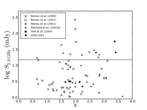
Figure 1: Distribution of known radio-loud BAL QSOs in log S and z before going on-sky. The sample to be studied in this paper was selected by taking all those with $S_{1.4\rm{GHz}}>$ 15 mJy.

At a later stage, Trump et al. (2006) presented a catalogue with 4784 SDSS BAL QSOs selected using a more homogeneous selection criteria. They used an automated algorithm to fit the continuum and measure the AI (Absorption Index, Hall et al. 2002) in all quasars from the SDSS-DR3 quasar catalogue (Schneider et al., 2005). In fact, all SDSS quasars in the RBQ sample belong to the list of Trump et al. (2006), except 0039-00 which is not included in the SDSS-DR3 quasar catalogue, but appears in the more recent SDSS-DR5 quasar catalogue (Schneider et al., 2007). However, some care has to be taken when using the list of Trump et al. (2006). According to the more subjective classification by Ganguly et al. (2007), the absorption present in about 15 per cent of the quasars classified as BAL QSOs in Trump’s list might actually be due to intervening systems instead of having an intrinsic origin. Some examples of these false positives are shown in Figure 2 of Ganguly et al. (2007).

In this work the radio spectra of BAL QSOs will be described, and in particular, the spectral index distribution will be compared with that of a non-BAL QSO sample. This is an interesting exercise because the spectral index is known to be an statistital indicator of the orientation of quasars, and this comparison can give some information about the orientation of BAL QSOs. This comparison sample of non-BAL QSOs has been extracted from the complete B3-VLA quasar catalogue (Vigotti et al., 1997). The B3-VLA survey (Vigotti et al., 1989) consists of 1049 sources selected from the B3 survey (Ficarra et al., 1985) in five flux density bins between declination 37 and 47 deg. It was designed to be complete down to flux densities of 100 mJy at 408 MHz. In addition to the original flux densities at 408 MHz the entire classical radio frequency range has been covered for most of the sources in the sample, both from already existent surveys (6C at 151 MHz, WENSS at 325 MHz, NVSS at 1400 MHz, GB6 at 4850 MHz) and from dedicated observations, mainly at higher frequencies (74 MHz, Mack et al. 2005; 2.7 GHz, Klein et al. 2003; 4.85 GHz, Vigotti et al. 1999 and 10.5 GHz, Gregorini et al. 1998). Based on this radio survey, Vigotti et al. (1997) presented a complete sample of 125 quasars and this will be used as a comparison sample of radio-loud non-BAL quasars.

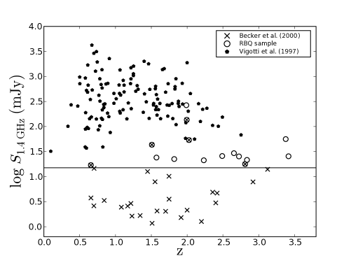
Figure 2: Same plot as Figure 1 in which the sample of normal radio-loud quasars from Vigotti et al. (1997) is shown, together with the samples of radio-fainter BAL QSOs.

In Figure 2 the flux density is plotted against the redshift but now the sample of Vigotti et al. (1997) is presented together with that of Becker et al. (2000) and the one studied in this paper. The redshift range covered by the BAL QSOs goes from 0.656 to 3.124 (Becker’s list) and to 3.416 (RBQ sample). The sources in Vigotti et al. (1997) list are, on average at smaller redshift ($z_{mean}$=1.25), but they cover the redshift range between 0.096 and 2.757. Figure 2 also illustrates how the RBQ sample represent intermediate flux densities, between the flux density coverage spanned by the relatively faint sample of (Becker et al., 2000) and that covered by the list of brighter quasars from Vigotti et al. (1997).

3 Observations and data reduction

Radio-continuum flux densities with full polarisation information were collected for the RBQ sample at different frequencies in several runs with the Effelsberg 100-m radiotelescope and the Very Large Array (VLA). A summary of the different observing runs can be found in Table 2, and the list of frequencies used with their characteristics (e.g., angular resolutions) are displayed in Table 3.

Table 2: Summary of the observations.

Run	Date	Telescope	Frequencies (GHz)
1	26$-$30 Jan 05	Effelsberg	4.85, 8.35, 10.5
2	15$-$16 Jul 05	Effelsberg	4.85, 8.35, 10.5
3	27 Oct 05	Effelsberg	4.85, 8.35, 10.5
4	23$-$26 Jun 06	Effelsberg	2.65
5	13 Feb 06	VLA(A)	8.45, 14.5, 22.5, 43.5
6	7 Mar 06	VLA(A)	8.45, 14.5, 22.5, 43.5

3.1 Effelsberg 100-m telescope

The single-dish observations at 4.8, 8.4 and 10.5 GHz took place in January 2005. Some sources were re-observed in July and October 2005 in order to confirm doubtful values or improve the signal-to-noise ratio. Observations at 2.65 GHz were carried out in June 2006. All receivers used in these observations are mounted on the secondary focus of the 100-m antenna. The recently installed 2.7-GHz hybrid feed can observe simultaneously in 9 channels, 8 of them 10-MHz wide and the ninth covering the full 80-MHz range. Since the sources in our sample are too faint to have a high signal-to-noise ratio per channel, only the wide-band channel centred at 2.65 GHz has been used. The receivers at 4.8 and 10.5 GHz have multi-feed capabilities with 2 and 4 horns, respectively, allowing real-time sky subtraction in every subscan measurement.

The observational strategy consisted of cross-scanning the source position in azimuth and elevation. These perpendicular scans were added to gain a factor $\sqrt{2}$ in sensitivity since the higher resolution FIRST maps ($\sim$ 5$\arcsec$) showed that none of these sources has structure more extended than 1 arcmin, the higher resolution in our observations (see Table 3). The cross-scan length was chosen to be about four times the beam size at each frequency for a correct subtraction of linear baselines. The scanning speed ranged from 8$\arcsec$ to 32$\arcsec$/s depending on the frequency, stacking typically 8 subscans at 2.65 GHz, and some 16 subscans in the rest of the frequencies (32 for the faintest sources at 10.5 GHz). This translates into on-source integration times between 15-75 sec per source and per frequency. Before combining, individual subscans were checked to remove those affected by radio frequency interference, bad weather, or detector instabilities.

The calibration sources 3C 286 and 3C 295 were regularly observed to correct for both time-dependent gain instabilities and elevation-dependent sensitivity of the antenna and to bring our measurements to an absolute flux density scale (Baars et al., 1977). The quasar 3C 286 was also used as a polarisation calibrator obtaining the polarisation degree $m$ and the polarisation angle $\chi$ in agreement with the values in the literature (Tabara & Inoue, 1980) within errors $<$1 per cent and $<$5 deg, respectively. The unpolarised planetary nebula NGC 7027 was also observed to have an estimation of the instrumental polarisation at each frequency.

The measurement of flux densities from the single-dish cross-scans was done by fitting Gaussians to the signal from all the polarimeter outputs (Stokes I, Q and U) and identifying the Gaussian amplitudes with the flux densities $S_{I}$, $S_{Q}$ and $S_{U}$. For all sources with significant $S_{Q}$ and $S_{U}$ contributions, the polarised flux density $S_{P}$, the degree of linear polarisation $m$ and the polarisation angle $\chi$ were computed, using the expressions given in Klein et al. (2003).

3.2 Very Large Array

VLA data were taken during February/March 2006 in the most extended A configuration using the receivers corresponding to the X, U, K and Q bands, i.e., at 8.4, 15, 22 and 43 GHz, respectively. Integration times were chosen on the basis of the predicted flux densities at these frequencies, after extrapolating from the Effelsberg frequencies with the adequate spectral indices. Those sources with indications of measurable polarised emission were observed more deeply and those expected to be too faint for this purpose were observed to have at least a good signal to noise ratio in $S_{I}$. Integration times range from $\sim$1 minute at 8.4 GHz up to $\sim$1 hour at 22 or 43 GHz for some sources.

At the two highest frequencies the fast-switch method was used, quickly switching between target and calibrator in order to have phase stability, taking care of the rapid atmospheric fluctuations. The duration of the cycles target-calibrator was of $\sim$ 150 to 200 seconds in the two highest frequencies.

3C 286 was the primary flux density calibrator and 3C 48 was used to test the goodness of the flux scale solution. Several phase calibrators chosen from the VLA calibrator manual were observed during the run. Most were selected at about 2-5 deg from their target sources, and in all cases within 10 deg. This is especially important to avoid the loss of coherence at the highest frequencies. Again the flux density scale is the one of Baars et al. (1977) except at 22 and 43 GHz where the Baars expressions are not valid. At these frequencies the adopted scale is based on emission models and observations of planet Mars, and is supposed to be accurate at a level of 5-10 per cent.

Table 3: Observing frequencies and beam sizes.

Telescope	Frequency	Bandwidth	$\theta_{\rm{HPBW}}$
	(GHz)	(MHz)	(arcsec)
Effelsberg	2.65	350	265
Effelsberg	4.85	500	145
Effelsberg	8.35	1200	80
Effelsberg	10.5	300	65
VLA(A)	8.45	700	0.24
VLA(A)	14.5	700	0.14
VLA(A)	22.5	2000	0.08
VLA(A)	43.5	10000	0.05

The 31DEC06 version of the AIPS package was used to flag, calibrate, clean and image the VLA data. The standard recipe was followed in all frequencies. However, at 22 and 43 GHz opacity and gain curve corrections were applied as a previous step to the standard calibration, and the calibration table was gridded in intervals of 3 seconds to get rid of rapid atmospheric fluctuations. The appropriate clean component models were used for 3C 286 and 3C 48 at these two frequencies. The peak flux densities were measured by fitting 2-D Gaussians to the source profiles. The integrated flux densities were computed using the BLSUM task, adding the signal in small boxes containing each source. The same boxes were used to measure the Stokes parameters S_Q and S_U. The local noise of the maps was estimated from a circular region around each individual source. Peak and integrated flux densities have essentially the same values because most sources are unresolved, as will be discussed below.

The polarisation calibration of the VLA data was determined using the AIPS tasks PCAL and RLDIF. The first solves for the feed parameters in each antenna, using repeated observations of a strong unresolved source (in our case several snapshots of 3C 286 were taken) covering a range of different parallactic angles. RLDIF determines and subtracts any phase difference between the right and left polarisation systems. The residual instrumental polarisation at the VLA frequencies was estimated measuring the linear polarisation of 3C 84 after having applied the polarisation calibration. Aller et al. (2003) report that this source shows a percentage of linear polarisation of 0.12 $\pm$ 0.01 at 14.5 GHz, and for our purposes it can be considered unpolarised.

3.3 Error determination

We consider three main contributions to the flux density error as in Klein et al. (2003). These are (i) the calibration error $\Delta S_{cal}$ (in percentage) which is estimated by the dispersion of the different observations of the flux density calibrators; (ii) the error introduced by noise, $\Delta S_{n,i}$, which is estimated from the local noise around the source; and (iii) the confusion error $\Delta S_{conf,i}$ due to background sources within the beam area. This last term can be neglected in interferometric data where the synthesised beam has small dimensions.

Thus the expressions for the total uncertainty of Stokes parameters are Equations 1 and 2 for Effelsberg and the VLA, respectively:

$$\Delta S_{i}=\sqrt{(S_{i}\cdot\Delta S_{cal})^{2}+\Delta S_{n,i}^{2}+\Delta S_{conf,i}^{2}}\hskip 14.22636pti={\rm I,Q,U}$$ (1)

$$\Delta S_{i}=\sqrt{(S_{i}\cdot\Delta S_{cal})^{2}+S_{n,i}^{2}\cdot\frac{A_{src}}{A_{beam}}}\hskip 14.22636pti={\rm I,Q,U}$$ (2)

where $A_{src}$ is the area of the box used to measure the source flux density, and $A_{beam}$ is the beam area. The expressions for the uncertainties of $S_{P}$, $m$ and $\chi$ can be taken from Klein et al. (2003).

Table 4: Values used to calculate the errors of the Stokes parameters and obtained instrumental polarisations.

Telescope	Frequency	$\Delta S_{conf}$		$\Delta S_{cal}$	$P_{instr}$
	(GHz)	(I)	(Q,U)	(per cent)
Effelsberg	2.65	1.5	0.5	0.8	0.7
Effelsberg	4.85	0.45	0.15	0.9	0.7
Effelsberg	8.35	0.23	$-$	1.0	0.6
Effelsberg	10.5	0.08	$-$	1.9	0.8
VLA	8.45	$-$	$-$	1.9	$<$0.1
VLA	15.0	$-$	$-$	2.9	0.6
VLA	22.5	$-$	$-$	1.8	0.7
VLA	43.5	$-$	$-$	5.3	2.1

Table 4 shows the coefficients used for the calculation of errors $\Delta S_{i}$. The confusion limits at 2.7, 4.8 and 10.5 GHz have been extracted from Klein et al. (2003) and that at 8.35 GHz (not available in Klein et al. 2003) was obtained from our own observations inspecting the behaviour of the signal rms at long integration times. This value is consistent with the interpolation over frequency from the two adjacent bands (at 4.85 and 10.5 GHz). The last column in Table 4 lists the instrumental polarisation for the different frequencies and telescopes.

4 Results

4.1 Radio flux densities

Tables 5 and 6 show the measured flux densities and errors (in mJy) between 74 MHz and 43 GHz for the RBQ sample. At frequencies below 2.6 GHz there are available flux densities from the literature and these are listed in Table 5. The flux densities at 325 MHz were obtained from the Westerbork Northern Sky Survey (WENSS; Rengelink et al. 1997). In addition, 3-$\sigma$ upper limits and a detection from the Texas survey (Douglas et al., 1996) at 365 MHz are given for those sources not covered by the WENSS survey. At 74 MHz none of the sources is detected in the VLA Low-Frequency Sky Survey (VLSS; Cohen et al. 2007), but 3-$\sigma$ upper limits have been computed measuring the local noise around the source position in the available images. Flux densities at 1.4 GHz from FIRST and NVSS (Condon et al., 1998) can be also found in Table 5.

The BAL QSO 1624+37 was observed in this campaign at 2.65 GHz with Effelsberg and at 15 and 43 GHz with the VLA. All the flux densities in the remaining frequencies were presented by Benn et al. (2005).

Table 5: RBQ sample of 15 radio-loud BAL QSOs: Flux densities (in mJy), errors or 3-$\sigma$ upper limits from 74 MHz to 1.4 GHz obtained from the literature.

ID	$S_{0.074}^{\rm{VLSS}}$	$S_{0.365}^{\dagger}$	$S_{1.4}^{\rm{FIRST}}$	$S_{1.4}^{\rm{NVSS}}$
0039$-$00	$<$475	$<$80	21.2	19.5 $\pm$ 0.7
0135$-$02	$<$350	$<$80	22.4	22.8 $\pm$ 1.1
0256$-$01	$<$385	$<$80	27.6	22.3 $\pm$ 0.8
0728+40	$<$300	15 $\pm$ 3.3†	17.0	17.2 $\pm$ 0.6
0837+36	$<$290	184 $\pm$ 3.4†	25.5	$-$
0957+23	$<$260	$<$80	136.1	136.9 $\pm$ 4.1
1053$-$00	$<$500	$<$80	24.7	22.7 $\pm$ 1.1
1159+01	$<$320	887 $\pm$ 30${}^{\leavevmode\nobreak\ \leavevmode\nobreak\ }$	268.5	275.6 $\pm$ 8.3
1213+01	$<$340	$<$80	21.5	27.5 $\pm$ 7.9
1228$-$01	$<$340	$<$80	29.4	29.1 $\pm$ 1.0
1312+23	$<$300	$<$80	43.3	46.5 $\pm$ 1.4
1413+42	$<$330	16 $\pm$ 3.2†	17.8	16.8 $\pm$ 0.6
1603+30	$<$225	33 $\pm$ 4.4†	53.7	54.1 $\pm$ 1.7
1624+37	$<$355	59 $\pm$ 4.0†	56.1	55.6 $\pm$ 1.7
1625+48	$<$290	26 $\pm$ 3.7†	25.3	26.0 $\pm$ 0.9

The symbol $\dagger$ indicate data from WENSS at 325 MHz, the rest are from the Texas Survey at 365 MHz.

Table 6: RBQ sample of 15 radio-loud BAL QSOs: Flux densities (in mJy) from 2.6 to 43 GHz obtained in this work. Superscripts on the errors indicate the run number of that observation, according to the key in Table 2. The exception is 1624+37 (with superscript 0), for which several flux densities were presented in Benn et al. (2005)

ID	$S_{2.6}$	$S_{4.8}$	$S_{8.3}$	$S_{8.4}$	$S_{10.5}$	$S_{15}$	$S_{22}$	$S_{43}$
0039$-$00	$-$	19.3 $\pm$ 0.61	12.0 $\pm$ 0.41	12.3 $\pm$ 0.15	9.7 $\pm$ 0.41	6.2 $\pm$ 1.15	2.2 $\pm$ 1.25	1.1 $\pm$ 0.15
0135$-$02	$-$	27.2 $\pm$ 0.61	31.9 $\pm$ 0.81	30.8 $\pm$ 0.45	29.5 $\pm$ 0.73	22.7 $\pm$ 0.85	14.7 $\pm$ 0.25	2.3 $\pm$ 0.25
0256$-$01	$-$	12.0 $\pm$ 0.51	7.2 $\pm$ 0.31	7.2 $\pm$ 0.45	5.9 $\pm$ 0.41	4.3 $\pm$ 1.55	2.2 $\pm$ 0.35	1.4 $\pm$ 0.15
0728+40	6.7 $\pm$ 1.54	6.4 $\pm$ 0.71	3.1 $\pm$ 0.21	2.5 $\pm$ 0.35	1.6 $\pm$ 0.31	1.9 $\pm$ 0.35	0.83 $\pm$ 0.065	$-$
0837+36	50.4 $\pm$ 1.64	30.2 $\pm$ 2.32	12.1 $\pm$ 0.81	12.5 $\pm$ 0.16	13.0 $\pm$ 0.42	3.3 $\pm$ 1.36	2.2 $\pm$ 0.56	1.3 $\pm$ 0.26
0957+23	93.7 $\pm$ 2.44	78.7 $\pm$ 1.11	48.5 $\pm$ 1.21	53.2 $\pm$ 0.55	39.8 $\pm$ 1.21	31.4 $\pm$ 0.75	22.4 $\pm$ 0.35	9.8 $\pm$ 0.95
1053$-$00	13.6 $\pm$ 1.64	15.7 $\pm$ 0.61	11.8 $\pm$ 0.41	13.1 $\pm$ 0.15	12.3 $\pm$ 0.61	8.2 $\pm$ 1.65	5.9 $\pm$ 0.75	2.3 $\pm$ 0.75
1159+01	133.9 $\pm$ 2.04	137.8 $\pm$ 1.71	158.0 $\pm$ 2.02	160.8 $\pm$ 1.25	150.6 $\pm$ 3.72	123.8 $\pm$ 1.65	105.5 $\pm$ 1.15	74.6 $\pm$ 2.15
1213+01	23.0 $\pm$ 1.74	15.2 $\pm$ 0.51	9.7 $\pm$ 0.31	11.6 $\pm$ 0.15	8.2 $\pm$ 0.51	5.6 $\pm$ 1.45	3.6 $\pm$ 0.55	1.4 $\pm$ 0.25
1228$-$01	19.4 $\pm$ 1.64	18.6 $\pm$ 0.51	15.5 $\pm$ 0.41	16.9 $\pm$ 0.25	13.5 $\pm$ 0.71	11.5 $\pm$ 1.65	8.1 $\pm$ 0.25	2.5 $\pm$ 0.75
1312+23	28.9 $\pm$ 1.64	25.7 $\pm$ 0.61	19.8 $\pm$ 0.51	19.4 $\pm$ 0.25	16.1 $\pm$ 0.61	10.5 $\pm$ 0.35	7.7 $\pm$ 0.16	5.4 $\pm$ 0.46
1413+42	7.6 $\pm$ 2.94	8.8 $\pm$ 0.72	13.4 $\pm$ 0.32	13.4 $\pm$ 0.16	12.7 $\pm$ 0.42	9.5 $\pm$ 1.56	7.0 $\pm$ 0.26	2.2 $\pm$ 0.46
1603+30	22.8 $\pm$ 1.74	26.1 $\pm$ 0.71	19.1 $\pm$ 0.51	22.1 $\pm$ 0.35	16.8 $\pm$ 0.61	12.5 $\pm$ 1.75	8.3 $\pm$ 0.15	1.9 $\pm$ 0.55
1624+37	33.5 $\pm$ 1.64	23.3 $\pm$ 1.10	$-$	15.0 $\pm$ 0.10	10.5 $\pm$ 0.80	9.6 $\pm$ 0.65	5.41 $\pm$ 0.020	2.1 $\pm$ 0.35
1625+48	17.6 $\pm$ 1.54	9.4 $\pm$ 0.72	8.0 $\pm$ 0.22	7.0 $\pm$ 0.25	6.3 $\pm$ 0.22	5.8 $\pm$ 1.35	1.9 $\pm$ 0.35	1.7 $\pm$ 0.25

4.2 Morphologies

The FIRST maps at 1.4 GHz show a compact morphology for all 15 BAL QSOs in the RBQ sample, at a resolution of $\sim$5$\arcsec$. To quantify this we have computed the morphological parameter $\Theta$, based on the FIRST integrated and peak flux densities, $\Theta$ = log(S_int/S_peak), and for all 15 sources $\Theta<$0.03. All sources, with the exception of 1053$-$00, appear essentially point-like at this resolution. The FIRST map of 1053$-$00 is shown in Figure 3 where a point-like core and two faint components (5- and 8-$\sigma$ detections) can be seen. The faint components seem to be real and this source has been included in the catalogue of double-lobed radio quasars from SDSS (de Vries et al., 2006). This is thus an additional example of the rare class of BAL QSOs showing double-lobed morphology, and it is not included in the list of 8 SDSS BAL QSOs of this type compiled by Gregg et al. (2006).

Our VLA maps at higher frequencies confirm the compactness of the 15 BAL QSOs, having all of them point-like structure at 8.4 and 15.0 GHz. The faint components of 1053$-$00 cannot be seen at these frequencies, probably due to a steep spectral index in these two regions.

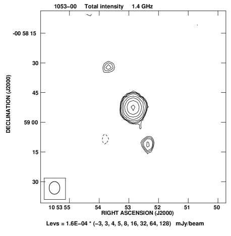
Figure 3: Map of BAL QSO 1053$-$00 from FIRST at 1.4 GHz. The synthesized beam-size is shown in the lower-left corner.

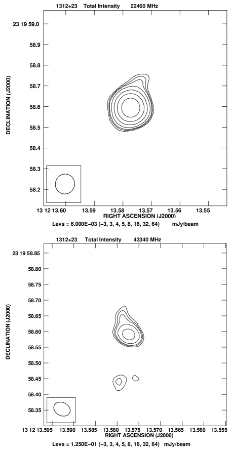
Figure 4: VLA map of BAL QSO 1312+23 at 22 GHz (top) and at 43 GHz (bottom). The synthesized beam-size is shown in the lower-left corner of each map.

The combination of the 43-GHz band with the A configuration provides the highest resolution available with the VLA ($\theta_{HPBW}\sim 50$ mas). However, as can be seen in Table 6 most sources are very faint at 43 GHz, i.e., close to the 1 mJy level. For those the self-calibration process is not appropriate and the way to recover the flux densities was to assume an initial point-source model before the first mapping. This procedure is to some extent well justified since at lower frequencies the morphology is still point-like, although the precise astrometric and morphological information about the sources at 43 GHz is lost.

Self-calibration at high frequency was only possible for the brightest sources: 0957+23, 1159+01 and 1312+23. The first two sources appear point-like in the 43-GHz maps. Figure 4 shows the naturally weighted maps of 1312+23 at 43 and 22 GHz, revealing an extension towards the north coming from the central unresolved component. Although the feature, possibly a jet, is detected at both frequencies, its significance is higher at 43 GHz.

The small feature in the 43-GHz map at $\sim$120 mas south from the central source is probably not real because it is located in a region affected by a stripe. It must be noticed that at this high frequency this flux density level is probably close to the limit where signal coherence allows accurate mapping. For the remaining 12 sources the mapping at 43 GHz was not possible and an upper limit on their sizes was obtained using the observations at 22 GHz ($\theta_{HPBW}\sim 80$ mas), where they are bright enough for mapping. For those, the task IMFIT was used to fit an elliptical Gaussian component and a zero level within a small box containing the radio source, yielding the major and minor axes of the fitted Gaussian, position angle and the formal beam-deconvolved dimensions. The uncertainty in the dimensions was estimated following Equation 1 of White et al. (1997). Eight of the twelve sources are clearly more extended than the beam size and their fitted parameters are given in Table 7. Also in this table are shown the dimensions of 1312+23 and 1624+37, as measured from the map in Figure 4 and from VLBA observations to be published in a subsequent paper, respectively. The remaining three sources (0039$-$00, 0256$-$01, 1053$-$00) plus 0957+23 and 1159+01 can be considered strictly unresolved at high frequencies.

Table 7: Angular dimensions for the extended sources.

Source	Freq.	$\theta_{maj}$	$\theta_{min}$	PA	$\theta_{maj}^{(dec)}$
	(GHz)	(mas)	(mas)	(deg)	(mas)
0135$-$02	22	112.4	78.7	$-$12	11 $\pm$ 4
0728+40	22	85.5	73.0	26	26 $\pm$ 6
0837+36	22	94.0	85.9	34	19 $\pm$ 10
1213+01	22	111.7	75.5	$-$19	27 $\pm$ 11
1228$-$01	22	95.3	76.3	$-$30	19 $\pm$ 4
1312+23	43	54.5	41.8	64	69 $\pm$ 12†
1413+42	22	92.0	69.5	$-$60	9 $\pm$ 3
1603+30	22	95.8	71.0	$-$71	15 $\pm$ 3
1624+37	4.8	$-$	$-$	$-$	36 $\pm$ 5††
1625+48	22	157.0	71.8	76	63 $\pm$ 20

$\dagger$ Not deconvolved size, but measured from the extended structure in Figure 4. $\dagger\dagger$ Measured from VLBA map at 4.8 GHz to be presented in Montenegro-Montes et al. (in prep.)

VLBI observations of 0957+23 and 1312+23 have been presented by Jiang & Wang (2003) using the European VLBI Network at 1.6 GHz. With a restoring beam of only 18.5 $\times$ 6.86 mas, 0957+23 appears as a single point-like component, while 1312+23 is resolved. This last source shows a symmetric morphology with a central core and two components in the northern and southern directions with a total extension of $\sim$150 mas (i.e., about 1 kpc). Although an extended morphology is also present in our 22-GHz and 43-GHz maps (Fig. 4), only the northern part is detected.

Summarising, our VLA maps show very compact morphologies for all 15 sources at all frequencies, at a maximum resolution of 80 mas. The exceptions are 1312+23 which shows some elongation at 22 and 43 GHz, and 1053$-$00 which is extended at 1.4 GHz showing two faint lobes not detected at higher frequencies.

4.3 Variability

We have checked for variability at 1.4 GHz comparing the flux densities from FIRST and NVSS epochs in those 14 sources with NVSS measurement. The same has been done at 8.4 GHz for those 5 sources in common with the list of Becker et al. (2000). They observed these sources with the VLA in A and D configuration (resolutions of 0.8 and 9 arcsec respectively) and all 5 sources presented point-like structure at both resolutions. As mentioned before this is again confirmed by our observations at 8.4 GHz in A configuration. This means that flux densities of both measurements can be directly compared. The same is true at 1.4 GHz because all sources except 1053$-$00 are point-like at the resolution of FIRST (B configuration) and the resolution of NVSS is poorer (VLA D and CnB configurations). Although 1053$-$00 is resolved, it has a compact nucleus and the two extensions are not expected to contribute much to the total flux density (Section 4.2).

We measure the flux density variations with the parameter $Var_{\Delta S}$, as defined e.g. by Torniainen et al. (2005):

$$Var_{\Delta S}=\frac{S_{max}-S_{min}}{S_{min}}$$ (3)

As an estimate of the significance of the source variability the $\sigma_{var}$ parameter defined by Zhou et al. (2006) is used, adopting the integrated flux densities $S_{1}$ and $S_{2}$ at the two epochs:

$$\sigma_{Var}=\frac{|S_{2}-S_{1}|}{\sqrt{\sigma_{2}^{2}+\sigma_{1}^{2}}}$$ (4)

where $\sigma_{2}$ and $\sigma_{1}$ are the uncertainties in the integrated flux densities. Table 8 shows flux densities, $Var_{\Delta S}$ and $\sigma_{Var}$ at 1.4 and 8.4 GHz, for those sources exhibiting $\sigma_{Var}>$ 3. For the flux densities of Becker et al. (2000), whose errors are not given in their work, a 5 per cent error is assumed.

A low percentage of the sample (only 2 out of 14 sources) shows variability at 1.4 GHz, both sources varying about 20 per cent and with a significance just above 3 standard deviations. At 8.4 GHz, 3 out of 5 sources are variable at this level and 1312+23 constitutes the most extreme case, showing variations of about 50 per cent with significance above 10.

Table 8: Sources showing significant flux density variability. At 1.4 GHz, $S_{1}$ comes from NVSS and $S_{2}$ from FIRST. At 8.4 GHz, $S_{1}$ comes from Becker et al. (2000), $S_{2}$ from this work (Table 6)

Source	Freq	$S_{1}$	$S_{2}$	$Var_{\Delta S}$	$\sigma_{Var}$
	(GHz)	(mJy)	(mJy)
0256$-$01	1.4	22.3$\pm$0.8 D	27.5 B	0.23	3.2
1213+01	1.4	27.5$\pm$0.9 D	22.9 B	$-$0.20	3.2
1312+23	8.4	12.6 A	19.4$\pm$0.2 A	0.54	10.3
1413+42	8.4	11.3 D	13.4$\pm$0.1 A	0.19	3.7
1603+30	8.4	18.1 A	22.1$\pm$0.3 A	0.22	4.2

Flux density variations have recently been used to constrain the orientation of several BAL QSOs. Zhou et al. (2006) and later Ghosh & Punsly (2007) found a few examples of BAL QSOs with variability as high as 40 per cent at 1.4 GHz between the NVSS and FIRST, i.e., in periods of about 1-5 years. These variations were high enough to make the brightness temperature $T_{B}$ exceed the $10^{12}$ K limit associated to the Compton catastrophe. This was interpreted as a sign of beaming and the jet was supposed to be oriented at a few degrees from the line of sight.

The same procedure can be applied to 0256$-$01 and 1213+01, accepting the 3-$\sigma$ significance as real. Following the formalism in Ghosh & Punsly (2007) and knowing that the time differences between the NVSS and FIRST observations are 2.1 and 3.4 years, respectively, the observed variations imply brightness temperatures of $T_{b}$=3.1$\cdot$10¹³ K for 0256$-$01 and 1.3$\cdot$10¹³ K for 1213+01. These translate into upper limits for the jet orientation angle with respect to the line of sight of $\sim$20 and 25 deg, respectively. One concern about this approach is that it is based on variability at a single frequency and from only two measurements. Moreover, the flux densities we obtained for 0256-01 at 8.4 GHz, with Effelsberg and almost one year later with the VLA, show a good match, i.e., 7.2$\pm$0.3 and 7.2$\pm$0.4 mJy respectively, in contradiction with the expected stronger variability at high frequencies.

4.4 Shape of the radio spectra

4.4.1 Sample of radio BAL QSOs

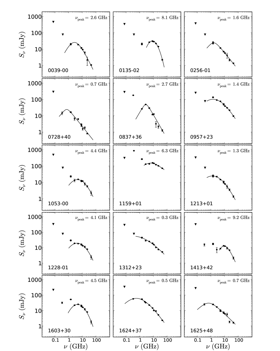
Figure 5: Radio spectra of the 15 BAL QSOs in the RBQ sample. Errors are shown if larger than the symbol size. Triangles mean 3-$\sigma$ upper limits. Solid lines are fits to the analytical function give in Section 4.4.1. The peak frequencies given at the top-right of each pannel were obtained from the fit. Some sources like 1159+01, 1413+42 and 1603+30 seem to have a second component at low frequencies.

Figure 5 show the spectra of the 15 objects. Many of them have a relatively steep spectrum at high frequency. About 75 per cent of the sample show flattening of the spectrum at low frequencies (typically below 1-5 GHz) which could indicate synchrotron self-absorption. However, in some cases some variability cannot be excluded, since the 1.4-GHz measurements were taken some years before the others. About 1/3 of the sample show, in addition, enhanced emission at MHz frequencies which could be indications of a second component emitting mostly in this range. Again, variability cannot be ruled out, but any possible time variability is expected to be less pronounced at lower frequencies. The source 1159+01 is the one which best fits in this category with both, a depression of the spectrum towards low frequency and a contribution from a second component in its spectrum.

Following the approach by Dallacasa et al. (2000), we have fitted each spectrum with the analytical function:

$$logS_{\nu}=a-\sqrt{b^{2}+(c\leavevmode\nobreak\ log(\nu)-d)^{2}}$$ (5)

where $a$,$b$,$c$,$d$ are numerical constants. This function, presented in Dallacasa et al. (2000) was used by these authors to obtain the frequency turnover, $\nu_{\rm{peak}}$, of sources with convex spectra peaking above a few GHz, referred to in that paper as High Frequency Peakers. The value of $\nu_{\rm{peak}}$ approximately marks the frequency region where the source starts to be optically thick to synchrotron radiation.

These fits have been done excluding some points in order to obtain a reduced $\chi^{2}$ below 0.05. This was possible for most of the sources which present a smooth radio spectrum, specially at high frequency, but not for 0728+40 ($\chi^{2}$=0.08) which presents a large scatter. At low frequencies, as we noted before, there are sources for which a possible second component arises. Again in these cases we decided whether to include or not in the fit these (low frequency) points trying to maintain the reduced $\chi^{2}$ within the mentioned limit. An exception was done with 0957+23 because even if an acceptable $\chi^{2}$ was obtained when including the 1.4 GHz flux densities, the resulting fit was not compatible with the 365 MHz upper limit.

In our sample we find 9 sources for which the spectrum peaks at a frequency higher than 1 GHz in the observer’s frame and there are 4 displaying a peak in the range 300-700 MHz. For the remaining three objects (0256$-$01, 0957+23 and 1312+23) the spectrum is slightly convex but not showing an obvious peak. However, power-law fits would not be compatible with the Texas upper limits and then extrapolated peaks compatible with both the spectrum curvature and these upper limits have been determined. The peak frequencies have to be multiplied by (1+z) to obtain intrinsic peak-frequencies.

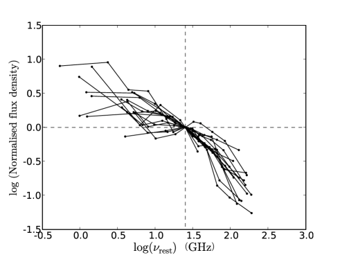
Figure 6: Rest-frame spectra of 15 BAL QSOs in the RBQ sample. They have been normalised to $\nu_{rest}$=25.0 GHz (log($\nu_{rest}$)=1.398)

In order to understand the global trends on the spectral shape of BAL QSOs, we compare in Figure 6 all the spectra bringing them first to the rest-frame in order to avoid the effect of the redshift. The rest-frame normalisation frequency was chosen to be 25 GHz. This is a compromise to choose a region representative of pure synchrotron emission, where neither synchrotron self-absorption nor synchrotron losses might be present in the majority of sources. This frequency also makes the dispersion of the normalised spectra relatively small compared to other normalisation frequencies.

We see in Figure 6 a variety of spectral slopes around 25 GHz. There is one object in the sample which differ more strongly from the main trend, This is 1413+42 which has a spectrum with two components separated at 4 GHz (see Figure 5), and for this reason it shows in Figure 6 an inverted spectrum around the normalisation frequency. Apart from this object, and assuming that variability effects are not very important, Figure 6 reflects the rest-frame spectrum of a typical BAL QSO in the RBQ sample. It is in general convex, quite flat below 10 GHz, and becoming steeper around 25 GHz. About half of the objects become even steeper at frequencies higher than 50 GHz.

The spectral shape can be quantified by means of the spectral indices. Table 9 provides the turnover frequencies and representative spectral indices at different frequencies, both in the observer’s and in the rest-frame. The spectral indices $\alpha_{0.365}^{1.4}$, $\alpha_{4.8}^{15}$ and $\alpha_{8.4}^{43}$ describe the low-, medium- and high-frequency regions. Moreover, the index $\alpha_{1.4}^{8.4}$ is shown for comparison with Becker et al. (2000). It is worth noting that the spectral indices $\alpha_{1.4}^{8.4}$ shown in Table 9 are not based on simultaneous observations, but as we previously have shown, variability might not be very important at this frequency, and in any case it only affects a small number of sources. In the rest-frame the indices $\alpha_{6.0}^{25}$, $\alpha_{12}^{25}$, $\alpha_{25}^{50}$ and $\alpha_{50}^{100}$ are also given in Table 9.

Looking at the rest-frame spectral indices of BAL QSOs and Figure 6, we see on average a flattening below 10 GHz, which is probably due to synchrotron self-absorption, and an overall convex shape. The low-frequency flattening is reflected in the median $\alpha_{6}^{25}$=$-$0.32, while the median $\alpha_{12}^{25}$ decreases to $-$0.57. The steepening at high frequency can be seen from the median $\alpha_{25}^{50}$ dropping to $-$0.92 and finally becoming steeper at higher frequencies with a median $\alpha_{50}^{100}$=$-$1.24.

The radio spectral index is known to be a statistical indicator of the orientation of radio sources (Orr & Browne, 1982). Becker et al. (2000) found respectively two thirds and one third of the radio-loud BAL QSOs in their list with steep and flat spectral index. However, it is worth to note that they define the limit between flat and steep to be $\alpha$=$-$0.5, and about one third of the sample has spectal index close to this value $-$0.6 $\leq\alpha\leq-$0.4. They suggest that this result is not consistent with BAL QSOs being oriented along a particular direction with respect to the line of sight to them. We find in our sample, which overlaps with that of Becker et al. (2000) in 5 objects, 60 per cent (9/15) of flat and 40 per cent of steep (6/15) spectrum sources, with 27 per cent of objects (4/15) being in the range $-$0.6 $\leq\alpha\leq-$0.4. These percentages are roughly consistent within the errors, which are large because the samples are relatively small.

Table 9: Turnover frequencies (in GHz) and spectral indices for the RBQ sample in the observer’s frame (columns 2-6) and the rest frame (columns 7-11). The spectral indices in the observer’s frame have been computed from each pair of observed flux densities while the rest-frame spectral indices are based on interpolation over the whole spectrum. Median values of the spectral indices are given in the last row.

	Observer’s frame					Rest frame
ID	$S_{peak}$	$\alpha_{0.365}^{1.4}$	$\alpha_{1.4}^{8.4}$	$\alpha_{4.8}^{15}$	$\alpha_{8.4}^{43}$	$S_{peak}$	$\alpha_{6.0}^{25}$	$\alpha_{12}^{25}$	$\alpha_{25}^{50}$	$\alpha_{50}^{100}$
(1)	(2)	(3)	(4)	(5)	(6)	(7)	(8)	(9)	(10)	(11)
0039$-$00	2.60	$-$	$-$0.30	$-$1.01	$-$1.48	8.45	$-$0.32	$-$0.54	$-$1.21	$-$1.88
0135$-$02	8.15	$-$	0.18	$-$0.16	$-$1.59	22.90	+0.17	+0.18	$-$0.70	$-$2.26
0256$-$01	1.60	$-$	$-$0.75	$-$0.91	$-$1.01	5.50	$-$0.74	$-$0.80	$-$0.90	$-$1.28
0728+40	0.70	+0.08	$-$1.07	$-$1.08	$-$	1.15	$-$0.88	$-$0.75	$-$	$-$
0837+36	2.70	$-$1.35	$-$0.40	$-$1.96	$-$1.39	12.00	$-$0.09	$-$1.00	$-$1.30	$-$2.16
0957+23	1.40	$-$	$-$0.52	$-$0.81	$-$1.04	4.25	$-$0.51	$-$0.60	$-$0.91	$-$1.09
1053$-$00	4.40	$-$	$-$0.35	$-$0.58	$-$1.07	11.15	$-$0.14	$-$0.30	$-$0.94	$-$1.31
1159+01	6.30	$-$0.81	$-$0.29	$-$0.09	$-$0.47	18.90	$-$0.09	+0.22	$-$0.44	$-$0.48
1213+01	1.30	$-$	$-$0.35	$-$0.88	$-$1.30	4.90	$-$0.35	$-$0.61	$-$1.02	$-$1.20
1228$-$01	4.15	$-$	$-$0.31	$-$0.43	$-$1.17	15.10	$-$0.29	$-$0.12	$-$0.55	$-$1.12
1312+23	0.35	$-$	$-$0.45	$-$0.79	$-$0.79	0.85	$-$0.43	$-$0.58	$-$1.01	$-$0.57
1413+42	9.20	+0.07	$-$0.16	+0.07	$-$1.11	35.05	$-$0.23	+0.45	$-$0.06	$-$1.04
1603+30	4.50	+0.33	$-$0.50	$-$0.65	$-$1.51	13.50	$-$0.29	$-$0.16	$-$0.98	$-$1.73
1624+37	0.55	$-$0.03	$-$0.74	$-$0.79	$-$1.21	2.40	$-$0.71	$-$0.64	$-$0.99	$-$1.00
1625+48	0.65	$-$0.02	$-$0.72	$-$0.43	$-$0.87	2.45	$-$0.76	$-$0.81	$-$0.41	$-$1.69
Median:		$-$0.02	$-$0.40	$-$0.79	$-$1.14		$-$0.32	$-$0.57	$-$0.92	$-$1.24

4.4.2 Comparison with non-BAL QSOs

To further investigate the question of the orientation of BAL QSOs we want to compare in this paper the spectral index distribution of quasars in a pure BAL QSO sample with that of a sample of non-BAL QSOs with the idea of interpreting possible differences with different orientations of both samples. In this comparison we will use the spectral range 1.4-8.4 GHz in the observer’s frame and 6.0-25 GHz in the rest frame.

The list of non-BAL QSOs will be that of Vigotti et al. (1997) presented in Section 2, but in all the following discussion we will restrict it to objects with z$>$0.5. This restriction only reduces the total number of objects from 124 to 119. We have computed the spectral indices in the same way as in our sample, considering pairs of observed flux densities in the observer’s frame and interpolating over the whole spectra in the rest frame. The spectral range covered by the non-BAL QSO sample goes from 74 MHz up to 10.5 GHz, and only those sources with z$>$1.5 will reach 25 GHz in the rest frame.

As a BAL QSO sample we will add to our RBQ sample the list of (Becker et al., 2000). They only provide flux densities in two frequencies, i.e., 1.4 and 8.4 GHz. Thus, combining these we end up with a combined sample of 38 BAL QSOs. These spectral indices can be found in Table 9 for objects in the RBQ sample, and in Table 2 of (Becker et al., 2000) for the remaining objects.

The Vigotti et al. sample could in principle contain both BAL QSOs and non-BAL QSOs. However, a low contamination of BAL QSOs is expected. Becker et al. (2001) showed that in the radio-powerful regime the fraction of BAL QSOs is small. They used the definition of radio-loudness parameter $R^{*}$ given by Stocke et al. (1992), i.e., the ratio of radio power at 5 GHz to optical luminosity at 2500 Å  in the rest frame. In the regime of QSOs with $log(R^{*})>$2 they estimated a fraction of 4 per cent ($<$1.5 per cent) of HiBAL (LoBAL) QSOs from the FBQS, in the interval of redshift [1.5,4.0] ([0.5,1.5]) where the C iv (Mg ii) absorbing features would be covered in optical spectra.

We have calculated $log(R^{*})$ for all quasars in Vigotti’s list. For this purpose, the radio luminosity at 5 GHz has been computed on the basis of the observed radio spectra, applying the appropriate K-correction interpolating between each pair of observed frequencies with the adequate spectral index. The optical luminosities at 2500 Å  were computed using the POSS-I APM E magnitudes published in Vigotti et al. (1997), but corrected from Galactic extinction following the maps of Schlegel et al. (1998) and assuming an optical spectral index of $\alpha_{opt}=-1$ ($S_{\nu}\propto\nu^{\alpha}$), which is the value adopted by Becker et al. (2001).

In Figure 7 the histogram shows how $log(R^{*})$ ranges from 1.9 to 4.6. To estimate the fraction of BAL QSOs following the mentioned proportions, we split this sample in two groups, one with 0.5$<$z$\leq$1.5 and the other with z$>$1.5, comprising 80 and 44 quasars respectively. About 1-2 HiBAL QSOs are expected in the high-z subsample and about 1 BAL QSO in the low-z subsample.

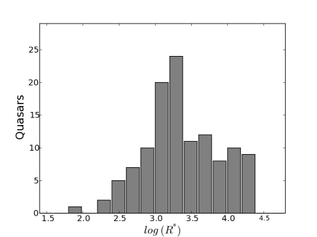
Figure 7: Histogram of radio-loudness parameter $R^{*}$ as defined by Stocke et al. (1992) for the sample of Vigotti et al. (1997).

We made use of the NASA Extragalactic Database (NED) and the SDSS-DR6 database to look for the optical spectra of QSOs from Vigotti et al. (1997) and check whether they are BAL QSOs. From 119 objects with z$<$0.5, 55 were found in the SDSS-DR6 database. These were inspected visually to look for the presence of BAL features. All of them are non-BAL QSOs and only one of them, (SDSS J080016.09+402955.6, associated to the radio source B3 0756+406) shows some broad absorption component bluewards of the C iv emission line, also present in Si iv. However, this absorption has a width of $\sim$ 1000 km s^-1 and it is located within 3000 km s^-1 from the line emission. It is therefore not consistent with the definition of BAL QSO but it could be better classified as a mini-BAL or a Narrow Absorption Line (NAL) system (see Figure 8).

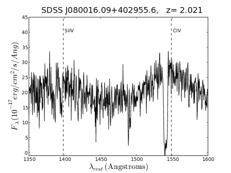
Figure 8: Spectrum of SDSS J080016.09+402955.6, showing a relatively narrow absorption in C IV and Si IV.

We searched for the remaining 64 spectra in the NED and found 14 of them in different publications, most of them in Vigotti et al. (1997) and Lahulla et al. (1991). From these 14, only 4 could be identified as normal QSOs without BALs: B3 0034+393 with z= 1.94 (Osmer et al., 1994); B3 0219+443 with z=0.85 (Djorgovski et al., 1990); B3 0249+383 with z=1.12 (Henstock et al., 1997) and B3 2351+456 with z=2.00 (Stickel & Kühr, 1993). The other 10 are difficult to classify because they are either faint, with low signal-to-noise ratio in the continuum (just good enough for a correct redshift identification), or the wavelength coverage does not include the region where the absorbing troughs could be present. Summing up, 59 out of 119 QSOs (roughly half of the sample) were inspected, with no one clearly showing the BAL phenomenon. These results justify the assumption that the list of (Vigotti et al., 1997) can be used as a representative sample of non-BAL quasars.

Table 10 summarises the number of elements and the basic statistics on the spectral index for the samples under comparison. Since BAL QSOs are compact objects as Becker et al. (2000) discovered and we confirm in this work, we will also consider in our comparison a subsample of non-BAL QSOs extracted from Vigotti et al. (1997) which includes only those compact sources with angular sizes $<$0.5 arcsec at 1.4 GHz. The angular sizes at 1.4 GHz in Vigotti’s sample were measured from maps taken with the VLA in C and D configurations (Vigotti et al., 1989) and for the most compact sources from observations in A configuration (priv. communication).

The first four rows in Table 10 show that non-BAL QSOs have a median $\alpha_{1.4}^{8.4}$ lower than BAL QSOs ($-$0.92 and $-$0.53, respectively). The conclusion could be that BAL QSOs tend to have flatter spectra and are, on average, oriented at a lower angle with respect to the line of sight than normal QSOs. On the other hand, when the non-BAL QSOs sample is restricted to compact objects only, the median spectral index becomes $-$0.49, very similar to that of BAL QSOs. When the full sample of non-BAL QSOs is considered, those extended objects have a higher contribution of emission produced in the lobes, which translates into steeper spectral indices for non-BAL QSOs. A similar behaviour can be found when analysing the rest-frame spectral indices $\alpha_{12}^{25}$ and also $\alpha_{6}^{25}$ although in this last case the median values for BAL QSOs and compact non-BAL QSOs are more distant, i.e. $-$0.32 and $-$0.47 respectively.

Table 10: Statistics on spectral indices. B00: Becker et al. (2000); V97: Vigotti et al. (1997); V97c: sources from Vigotti et al. (1997) with sizes $<$5 arcsec at 1.4 GHz

Sample	N	Min	Max	Mean	Median	Std
Observer’s frame: $\alpha$ [1.4 $-$ 8.4] GHz
RBQ+B00	38	$-$1.50	0.70	$-$0.50	$-$0.53	0.43
RBQ	15	$-$1.19	0.20	$-$0.52	$-$0.44	0.34
V97	119	$-$1.47	0.86	$-$0.80	$-$0.92	0.43
V97c	50	$-$1.41	0.86	$-$0.53	$-$0.49	0.49
Rest frame: $\alpha$ [6.0 $-$ 25] GHz
RBQ	15	$-$0.87	0.17	$-$0.38	$-$0.32	0.30
V97	51	$-$1.27	0.17	$-$0.71	$-$0.82	0.38
V97c	27	$-$1.21	0.17	$-$0.53	$-$0.47	0.40
Rest frame: $\alpha$ [12 $-$ 25] GHz
RBQ	15	$-$1.00	0.45	$-$0.40	$-$0.58	0.43
V97	51	$-$1.39	0.39	$-$0.71	$-$0.76	0.42
V97c	27	$-$1.31	0.39	$-$0.54	$-$0.62	0.44

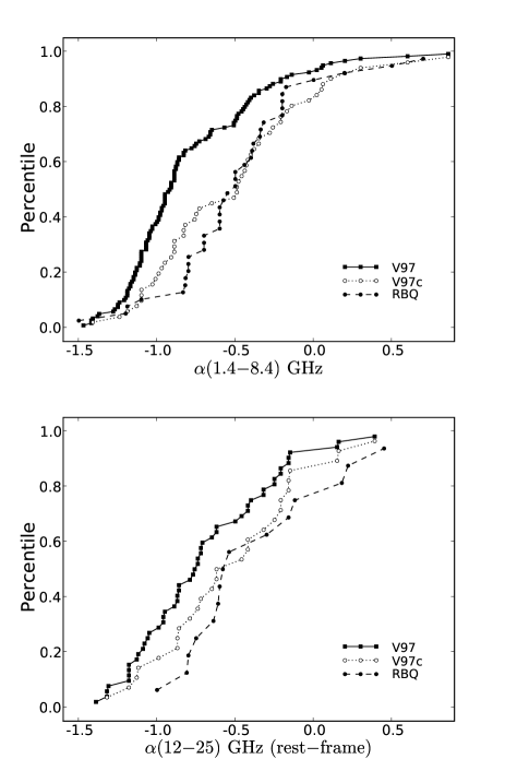
Figure 9: Percentile plot of the samples involved in the K-S tests, illustrating the shape of the spectral index distributions.

A Kolmogorov-Smirnov (K-S) test has been done in order to compare the $\alpha_{1.4}^{8.4}$ spectral index distributions of these samples. The test yields a probability P$<$0.001 that both distributions are statistically equal, confirming that they are indeed different populations. A similar K-S test restricted to only compact sources from Vigotti et al. (1997) yields P=0.204 which is consistent with both samples having a similar distribution. The percentile plot in the upper panel of Figure 9 illustrates the shape of the spectral index distribution of these three samples. It can be seen that the important contribution of extended sources from Vigotti et al. (1997) makes the percentile curve rise more rapidly than in the other samples. This result essentially means that the differences in spectral indices between BAL and non-BAL QSOs arise only because BAL QSOs are compact sources, while normal QSOs include both compact and extended.

We will also compare the rest-frame spectral indices indices to look for possible intrinsic variations between BAL and non-BAL QSOs, once the redshift effect has been corrected for. The most reasonable comparison is using $\alpha_{12}^{25}$ where the effect of synchrotron self-absorption seem less pronounced. Two K-S tests have been done comparing these samples. The first compares Vigotti’s sources and RBQ yielding P=0.048, while the second compares only the compact sources in Vigotti et al. (1997) and RBQ, yielding P=0.629. Again we can talk about statistically different populations when all QSOs are included in the comparison, but not when only spectral indices of compact sources are compared. The percentile plot is shown in the lower panel of Figure 9.

Even if the previous statistical test are consistent with similar spectral index distributions for BAL QSOs and non-BAL compact sources, it is interesting to note in Figure 9 that there might be a small deficit of steep sources among BAL QSOs with spectral index $\sim-$0.7, compared to the compact sources in Vigotti et al. (1997). This effect is more marked in the upper panel, but also insinuated in the lower panel where, nevertheless, the number of objects is significantly smaller.

4.5 Polarisation

Table 11: Degree of polarisation, $m_{\nu}$ (in percentage), at several frequencies, $\nu$ (in GHz), for the RBQ sample. Most of the values are 3-$\sigma$ upper limits and those showing a measured value can have a relatively large error but come from an at least 3-sigma detection in Stokes Q or Stokes U. The BAL QSOs 1159+01 and 1624+37 presented separately (see Table 12 in this paper and Table 2 from Benn et al. 2005) are the only two sources with significantly detected polarisation.

ID	$m_{1.4}^{a}$	$m_{2.6}$	$m_{4.8}$	$m_{8.3}$	$m_{8.4}$	$m_{10.5}$	$m_{15}$	$m_{22}$	$m_{43}$
(1)	(2)	(3)	(4)	(5)	(6)	(7)	(8)	(9)	(10)
0039$-$00	$<$ 1.59	$-$	$<$ 3.8	$<$ 14.5	$<$ 0.67	$<$24.8	$<$10.5	$<$14.7	$<$ 8.3
0135$-$02	$<$ 1.26	$-$	$<$ 3.1	$<$ 5.0	$<$ 0.87	$<$ 8.6	3.9$\pm$4.0	$<$ 1.7	$<$ 7.4
0256$-$01	$<$ 1.41	$-$	$<$ 4.5	$<$ 26.4	$<$ 3.9	$<$16.4	$<$ 1.7	$<$22.7	$<$ 7.2
0728+40	$<$ 1.17	$-$	$<$17.5	$<$ 30.7	$<$ 10.1	$-$	$<$10.9	$<$ 5.1	$-$
0837+36	$-$	$<$ 27.9	$<$ 2.2	$<$ 6.9	$<$ 0.6	$<$16.4	$<$27.8	$<$15.2	$<$10.1
0957+23	$<$ 1.23	$-$	$<$ 0.7	$<$ 1.8	$<$ 0.5	$<$ 3.4	$<$ 0.9	2.0$\pm$1.4	$<$ 5.6
1053$-$00	$<$ 1.29	$-$	$<$ 4.2	$<$ 18.1	1.3$\pm$1.0	$<$20.8	$<$12.8	$<$ 7.3	$<$22.1
1213+01	$<$ 1.29	$-$	$<$ 5.4	$<$ 13.7	$<$ 0.5	$<$37.1	$<$19.0	$<$ 9.9	$<$ 7.3
1228$-$01	$<$ 1.35	$-$	$<$ 4.3	$<$ 10.7	$<$ 0.5	$<$24.6	$<$10.9	$<$ 1.0	$<$23.7
1312+23	$<$ 1.17	$-$	$<$ 2.5	$<$ 8.2	2.7$\pm$0.7	$<$16.2	$<$ 1.5	3.6$\pm$2.3	$<$ 6.5
1413+42	$<$ 1.26	$-$	$<$ 6.7	$<$ 8.9	$<$ 0.5	$<$15.5	$<$10.2	$<$ 1.1	$<$ 9.5
1603+30	$<$ 1.32	$<$ 19.3	$<$ 2.4	$<$ 5.8	1.0$\pm$1.0	$<$14.0	$<$11.2	$<$ 0.8	$<$19.3
1625+48	$<$ 1.08	$<$ 24.0	$<$ 6.4	$<$ 7.4	$<$ 4.9	$<$16.6	$<$19.9	$<$19.8	17.6$\pm$14.0

^a Degree of linear polarisation at 1.4 GHz extracted from the NRAO VLA Sky Survey, NVSS (Condon et al., 1998)

The RBQ sample was searched in the NVSS database looking for polarised emission and only one BAL QSO, 1159+01, shows a high amount of linear polarisation at 1.4 GHz. For the rest of the sources only upper limits could be established typically below 1.5 per cent at this frequency.

At higher frequencies and up to 43 GHz we have measured the $S_{Q}$ and $S_{U}$ parameters as explained in Section 3, in order to obtain the degree of linear polarisation, $m$, and the polarisation angle $\chi$. Table 11 shows the fractional polarised intensity, mostly upper limits, for the BAL QSOs in the RBQ sample. The only sources which are clearly polarised showing significant $m$ at various frequencies are 1159+01 and 1624+37. These sources are presented in different tables (Table 12 in this paper and Table 2 from Benn et al. 2005). These two are the only bright sources displaying relatively high (i.e., $>$10 percent) polarised intensity at some frequency, having 1159+01 m_1.4=15 per cent and 1624+37 with m_10.5=11 per cent. Apart from these, also the weak source 1625+48 with only 1.7 mJy at 43 GHz shows m${}_{43}\sim$18 per cent but this measurement is based on a $\gtrsim$ 3-$\sigma$ detection in S_U and the uncertainty in this measurement is high. From the remaining sources in Table 11, 1312+23 shows significant polarisation at 8.4 and 22 GHz, and there are 5 more sources with significant detections at only one frequency, in all cases below 4 per cent.

It should be noted from Table 11 that the most stringent upper limits are given by the VLA observations at 8.4 GHz. At this frequency the sources are bright enough to have reliable detections and the relatively low noise achieved makes possible the determination of reasonable upper limits for the non-detections. At higher frequencies this is more difficult because the total power spectra drops down to fainter levels.

At 8.4 GHz, one third of the sample (i.e, 5 out of 15) show at least a 3-$\sigma$ detection in $S_{Q}$, $S_{U}$ or both. From these 5 BAL QSOs only 1624+37 is strongly polarised showing 6.5 per cent of linearly polarised flux density (Benn et al., 2005). The fractional polarised intensity in the other four objects (1053$-$00, 1159+01, 1312+23 and 1603+30) is below 3 per cent. The upper limits for most of the 10 undetected sources are below 1 per cent indicating strong depolarisation.

For 1159+01 and 1624+37 it is possible the determination of the Rotation Measure, RM, ($\chi=\chi_{0}+RM\cdot\lambda^{2}$) fitting a slope to the polarisation angles $\chi_{i}$ as a function of the square of the observed wavelenghts. Benn et al. (2005) already reported for 1624+37 a Rotation Measure of $-$990 $\pm$ 30 rad m^-2, which in the rest-frame translates into the extremely high intrinsic Rotation Measure, RM = -18350 $\pm$ 570 rad m^-2. For 1159+01 we have fitted the angles $\chi_{i}$ in Table 12. Our observations give a poor upper-limit at 2.65 GHz, but an additional measurement at this frequency has been obtained by Simard-Normandin et al. (1981). We get a best fit with a Rotation Measure RM=($-$72.1 $\pm$ 1.4) rad m^-2 and an intrinsic polarisation angle $\chi_{0}=-$24 $\pm$ 3 deg. This observed value should be corrected by the RM introduced by our own Galaxy, which is quite difficult to estimate. To have a rough estimate we have inspected the all-sky map presented by Wielebinski & Krause (1993) where the RM of 976 extragalactic sources are plotted. The neighbouring sources around the position of 1159+01 have small (i.e., $|$RM$|<$30 rad m^-2) Rotation Measures, which suggests that the Galactic contribution might be smaller than the determined value. Assuming no Galactic correction, the fitted Rotation Measure brought to the rest-frame would be higher by a factor (1+z)² becoming RM=(644 $\pm$ 12) rad m^-2.

Table 12: Polarisation properties of BAL QSO 1159+01. The second measurement at 2.65 GHz comes from Simard-Normandin et al. (1981)

Frequency	Telescope	$m$	$\chi$
(GHz)		(per cent)	(deg)
1.40	NVSS	15.03 $\pm$ 0.44	$-$31.1 $\pm$ 0.6
2.65	Effelsberg	$<$16	$-$
2.65	$-$	3.1 $\pm$ 1.9	111 $\pm$ 17
4.85	Effelsberg	2.1 $\pm$ 0.2	$-$42 $\pm$ 6
8.35	Effelsberg	0.95 $\pm$ 0.05	$-$29 $\pm$ 5
8.45	VLA	0.9 $\pm$ 0.4	$-$29 $\pm$ 7
10.5	Effelsberg	$<$1.2	$-$
15.0	VLA	$<$1.2	$-$
22.5	VLA	$<$0.4	$-$
43.5	VLA	$<$1.2	$-$

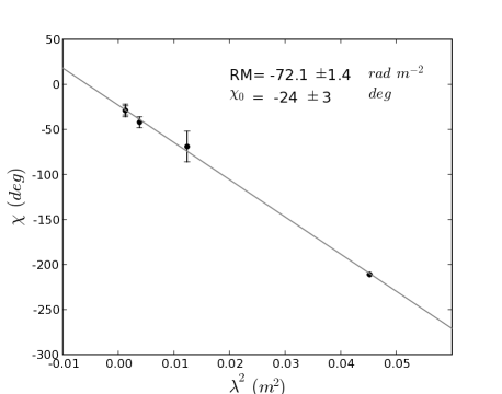
Figure 10: Determination of the RM for 1159+01.

5 Discussion

The morphologies and dimensions of the radio sources in BAL QSOs seem to be the keys to understand the orientation and evolutionary status of these sources. There is evidence that BAL QSOs are associated with compact radio sources, which are supposed to constitute a high fraction of the young population of radio sources, like e.g., CSS or GPS sources. Becker et al. (2000) noted that 90 per cent of their sample of radio-loud BAL QSOs (extracted from the FBQS survey) present point-like structure at the resolution of 5$\arcsec$ in contrast to the diversity of both point-like and extended sources they found within the whole population of FBQS quasars. In fact, only a few BAL QSOs are known to have an extended FR II radio structure (Gregg et al., 2006). Our 22-GHz observations of the RBQ sample confirm this tendency, because most sources appear unresolved at all frequencies constraining their apparent dimensions up to $\lesssim$0.1 arcsec. This translates into projected linear sizes (LS) $\lesssim$ 1 kpc which are typical of GPS/CSS sources. It could be argued that an extended component with a steep spectrum might be present, observable only at lower frequencies, and thus being the source sizes larger than those found at high frequencies. This hypothesis is a priori no supported by the fact that most sources are still point-like at 1.4 GHz as can be seen in the FIRST maps, with the exception of 1053$-$00.

The radio spectra in Figure 5 also display the typical convex shape of GPS-like sources, in most cases with a peak at $\sim$ 0.5$-$10 GHz suggested by at least one or two points, or by upper limits at MHz frequencies. One concern about this result is that FIRST or WENSS flux densities were observed at different epochs and variability might be an issue, although noticeable flux density variations are likely to be stronger in the optically thin region of the spectrum. However, relatively deep integrations at MHz frequencies would be desirable to better constrain the shape of the spectra at low frequency. In addition, a project with VLBI multi-frequency observations and the analysis on the pc-scale properties of several BAL QSOs of the RBQ sample has been started by us, and results will be presented in a subsequent paper.

If radio sources associated to BAL QSOs are actually CSS/GPS sources, they should follow the anticorrelation between intrinsic turnover frequency and projected linear size found by Fanti et al. (1990) for CSS sources. This was, for instance, quantified by O’Dea & Baum (1997) in a combined sample of CSS and GPS sources compiled by Fanti et al. (1990) and Stanghellini (1992), respectively. This relationship was found to be valid for both galaxies and quasars. The anticorrelation suggests that the mechanism producing the turnover simply depends on the source size. Figure 11 shows the relationship between intrinsic $\nu_{peak}$ and projected LS for the samples of CSS and CPS sources mentioned before, and we have also plotted for comparison our sample of radio-loud BAL QSOs. The turnover frequencies for the BAL QSOs appear in Table 9 while projected linear sizes have been extracted from the deconvolved sizes in Table 7.

A group of 5 BAL QSOs match quite well the distribution of CSS/GPS sources, and they all show simple convex spectra, i.e., 0728+40, 1213+01, 1312+23, 1624+37 and 1625+48. The three additional BAL QSOs displaying simple convex spectrum, 0039$-$00, 0256$-$01 and 0957+23 are unresolved in our observations and their position can only be constrained by upper limits. Nevertheless these 8 sources with simple complex spectrum are consistent with the correlation.

From the remaining 7 objects, 5 are resolved in our observations (0135$-$02, 0837+36, 1228$-$01, 1413+42 and 1603+30) and they are located above the cloud of CSS/GPS sources. All of them have in common a complex spectrum with indications of a double component. In these sources the turnover has been determined using the high frequency component but it is possible in the spectra of 1413+42 and 1603+30 to fit a second peak at lower frequencies (at 0.7 and 0.8 GHz respectively). A second peak at low frequency could also be fitted to 1159+01 but we will not do that because being this source unresolved we cannot give the exact location in the diagram. When considering the low frequency peaks of 1413+42 and 1603+30 in the diagram, these two sources also agree very well with the anticorrelation as shown in Figure 11. This better agreement could mean that the high-frequency part of these spectra could be dominated by the emission coming from a compact and active (possibly beamed) region smaller than the entire source, like a hot-spot. Unfortunately we do not have enough data to check whether this could be the case also for 0135-02, 0837+36 and 1228-01. Low-frequency data will be important to sample this part of the spectra to search for a possible second peak. Again, VLBI observations are crucial to further investigate this interpretation.

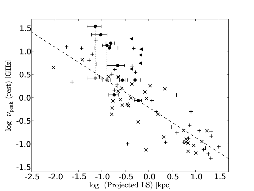
Figure 11: Rest-frame turnover frequency versus projected linear size relation for samples of CSS and GPS sources (adapted from O’Dea & Baum 1997). Galaxies are represented by the symbol ’$\times$’, quasars by the simbol ’+’ and the RBQ sample is plotted as solid circles. Upper limits for those BAL QSOs unresolved at 22 or 43 GHz are marked by triangles. The dashed line represent the anticorrelation found by O’Dea & Baum (1997): log $\nu_{peak}$ = $-$0.21$-$0.65 log LS. In those two resolved sources with two peaks in the spectrum (1413+43 and 1603+30) the grey points indicate the new location in the plot when the lower frequency peak is considered.

In fact, it has been shown that some GPS sources associated to optical QSOs can be just normal flat-spectrum quasars for which a jet/knot/hot-spot dominates the spectrum, which then adopts the characteristic convex shape of a GPS source, as discussed e.g. by Snellen et al. (1999). Recently Stanghellini et al. (2005) and Orienti et al. (2006) have studied VLBI samples of GPS sources and High Frequency Peakers (HFP, 5 GHz $<\nu_{\rm{pk}}<$ 10 GHz) confirming this scenario. In fact, these “contaminant” quasars seem to be present, even in high percentages, in many well-defined samples of GPS sources (Torniainen et al., 2005). Two characteristics of “genuine” young GPS radio sources are low polarisation and low variability (O’Dea, 1998), while flat-spectrum quasars show higher polarisation and variability.

Torniainen et al. (2005), who have used an extensive database of sources with multifrequency data from several long-term variability programs, define as “bona fide” GPS sources those with a maximum variability $Var_{\Delta S}<$3. From our comparison in Section 4 which is, of course, based on only two epochs we see that many sources do not show significant variations at 1.4 GHz, and 3 out of 5 inspected at 8.4 GHz show significant but not very strong variations. We cannot thus exclude these sources from the candidates to young sources. As also shown in Torniainen et al. (2005) the maximum variations are found at high frequencies, so multi-frequency multi-epoch observations of the RBQ sample will be very interesting for a more precise variability study.

Compact GPS sources are supposed to be completely embedded in their narrow line region. On this basis, (Cotton et al., 2003) proposed the existence of a typical frequency-dependent scale, below which the GPS source becomes completely depolarised, the so-called “Cotton effect”. Fanti et al. (2004) and later Rossetti et al. (2008) have confirmed this behaviour analysing the polarisation properties of the B3-VLA CSS sample (Fanti et al., 2001), and they propose models to describe the depolarising screen. The BAL QSOs in the RBQ sample have probably physical sizes of $\lesssim$ 1 kpc and if Faraday effects are important they should be completely depolarised even up to relatively high frequencies. This is the case for all sources except 1159+01 at 1.4 GHz, and also for about 70 per cent of the sample at 8.4 GHz. At these two frequencies the upper limits obtained for the degree of linear polarisation are reasonably small. From Table 11 only 1312+23 seems to be weakly polarised at 8.4 and 22 GHz, but no polarisation was found at 15 GHz.

The two exceptions are 1159+01 and 1624+37. The first source is weakly polarised at 8.4 GHz but it is worth to note that the degree of linear polarisation increases as frequency decreases, becoming strongly polarised at 1.4 GHz. The opposite is expected when a depolarising plasma curtain is present. The reason for this anomalous behaviour might be that the emission at low frequencies arises from a different component, as suggested by the complex radio spectrum (see Figure 5). An hypothetical extended structure with a relatively ordered magnetic field would contribute with substantial linear polarisation, and this may only be detected at low frequencies if a steep spectral index is assumed for the emission of this extended component.

The moderate observed Rotation Measure of ($-$72.1 $\pm$ 1.4) rad m^-2 in 1159+01 is consistent with the fact that it is strongly polarised in the NVSS. Should the Rotation Measure be much higher, the large bandwidth used for the NVSS observations would produce a strong bandwidth depolarisation effect, probably hiding any measurable polarised intensity. The extreme Rotation Measure of J1624+37, RM=$-$18350 rad m^-2 (Benn et al., 2005) which is the second highest value known among QSOs and the highest among BAL QSOs, seems to be an exception and not representative of the BAL QSOs family.

The median $m_{8.4}$ of the 5 polarised BAL QSOs in the RBQ sample is $\sim$1.3 per cent, but the remaining 10 BAL QSOs show $m_{8.4}\lesssim$1. As a comparison Saikia et al. (1987) found a median polarisation degree at 6 GHz of about 2 per cent in a subsample of quasars extracted from the sample of $\sim$400 compact sources of Perley (1982). Saikia et al. (1987) found no significant differences between the median value of flat-spectrum cores and CSS quasars whereas that radio sources associated to galaxies or to empty fields (no optical identifications) were found to be less polarised at 6 GHz, with a median value of $\sim$0.5 per cent. More recently, Stanghellini (2003) found a mean fractional polarisation of 1.2 and 1.8 per cent for GPS and flat-spectrum quasars, respectively, and $m<$ 0.3 per cent for galaxies.

The sources showing some polarisation in the RBQ sample have probably polarised intensities consistent with flat-spectrum quasars. It is also likely that some of them (e.g., 1159+01 or 1603+30) can show polarised emission due to Doppler boosted knots in jets, which is again compatible with their multi-component radio spectra peaking at high frequencies. However, our whole sample seem to be in better agreement with the GPS class than with the class of flat-spectrum quasars, because of the high percentage of unpolarised or weakly polarised sources. Of course, to firmly test this hypothesis it will be particularly interesting to do polarimetric multi-frequency observations of a radio brighter sample, which is now available after the recent releases of SDSS.

As far as the spectral index distribution is concerned, the different statistical tests suggest that the spectral index distributions of BAL and non-BAL QSOs are different. This difference is however due to the fact that all BAL QSOs in the sample have compact structures, while non-BAL QSOs have both extended and compact morphologies. When comparing the samples of BAL QSOs and compact non-BAL QSOs, no significant differences are found in the spectral index distributions. Thus, from our comparison no preferred orientation can be attributed to BAL QSOs. When larger samples become available, the comparison of spectral indices of BAL and non-BAL QSOs as a function of radio power and UV luminosity will be possible, allowing us to look for particular orientations in different bins of luminosity, as has been suggested by Elvis (2000).

6 Conclusions

• A sample of 15 BAL QSOs associated with FIRST sources brighter than 15 mJy has been built. Radio continuum observations for these sources have been collected from 2.6 up to 43 GHz in full polarisation. Flux densities covering this radio range have been presented complemented by archive data at lower frequencies from 74 MHz up to 1.4 GHz.

• VLA maps in the most extended configuration show very compact morphologies for most sources at all frequencies being unresolved or slightly resolved at 22 GHz with a resolution of 80 mas. These translate into projected linear sizes $\lesssim$ 1 kpc, which are the typical sizes of CSS/GPS sources.

• The spectra of these sources are typically convex, i.e., they seem to become flat or inverted at MHz frequencies probably due to synchrotron self-absorption, while at frequencies higher than 15 GHz they are definitely steeper. The spectra typically peak between 1 and 5 GHz in the observer’s frame and about 1/3 of the sample shows complex spectra suggesting different components.

• All BAL QSOs in our sample presenting simple convex spectra follow the anticorrelation between projected linear size and turnover frequency found for CSS and GPS sources. Two BAL QSOs with complex radio spectra are also in agreement with this relationship if we consider the lower frequency peak of their spectra. The higher frequency peak might be in this two sources due to emission from a hot-spot or a knot in a jet.

• A high percentage of the sample does not show significant variability when comparing the flux densities in 2 different epochs. Some BAL QSOs show significant variability at 8.4 GHz but not strong enough to exclude them from the candidates to young radio sources.

• Most BAL QSOs in our list are not strongly polarized either at 1.4 GHz or at 8.4 GHz, and sensible upper limits are given at these frequencies. Only two sources show significant polarisation at several frequencies. From these two, only the unusual BAL 1624+37 has a high Rotation Measures suggesting strong depolarization. The median fractional polarisation of the sample is in better agreement to mean values found in CSS/GPS sources, than those found for flat-spectrum quasars.

• A series of statistical tests have been done to compare the spectral index distribution of BAL and non-BAL QSOs finding that these distributions are different. However, no significant differences were found when comparing to compact non-BAL QSOs only. This is consistent with BAL QSOs spanning the same range of orientations as normal quasars with respect to our line of sight to them.

References

- Aller et al. (2003) Aller M.F., Aller H.D., Hughes P.A., 2003, ApJ, 586, 33
- Baars et al. (1977) Baars J.W.M., Genzel R., Pauliny-Toth I.I.K., Witzel A., 1977, A&A, 61, 99
- Becker et al. (1995) Becker R.H., White R.L., Helfand D.J., 1995, ApJ, 450, 559
- Becker et al. (2000) Becker R.H., White R.L., Gregg M.D., Brotherton M.S., Laurent-Muehleisen S.A., Arav N., 2000, ApJ, 538, 72
- Becker et al. (2001) Becker R.H. et al., 2001, ApJS, 135, 227
- Benn et al. (2005) Benn C.R., Carballo R., Holt J., Vigotti M., González-Serrano J.I., Mack K.-H., Perley R.A., 2005, MNRAS, 360, 1455
- Cohen et al. (2007) Cohen A.S., Lane W.M., Cotton W.D., Kassim N.E., Lazio T.J.W., Perley R.A., Condon J.J., Erickson W.C., 2007, AJ, 134, 1245
- Condon et al. (1998) Condon J.J., Cotton W.D., Greisen E.W., Yin Q.F., Perley R.A., Taylor G.B., Broderick J.J., 1998, AJ, 115, 1693
- Cotton et al. (2003) Cotton W.D. et al., 2003, PASA, 20, 12
- Dai et al. (2008) Dai X., Shankar F., Sivakoff G.R., 2008, ApJ, 672, 108
- Dallacasa et al. (2000) Dallacasa D., Stanghellini C., Centoza M., Fanti R., 2000, A&A, 363, 887
- de Vries et al. (2006) De Vries W.H., Becker R.H., White R.L., 2006, AJ, 131, 666
- Douglas et al. (1996) Douglas J.N., Bash F.N., Bozyan F.A., Wolfe C., 1996, AJ, 111, 1945
- Djorgovski et al. (1990) Djorgovski S., Thompson D.J., Vigotti M., Grueff G., 1990, PASP 102, 113
- Elvis (2000) Elvis M., 2000, ApJ, 545, 63
- Fanti et al. (1990) Fanti R., Fanti C., Schilizzi R.T., Spencer R.E., Rendong N., Parma P., van Breugel W.J.M., Venturi T., 1990, A&A, 231, 333
- Fanti et al. (1995) Fanti C., Fanti R., Dallacasa D., Schilizzi R.T., Spencer R.E., Stanghellini C., 1995, A&A, 302, 317
- Fanti et al. (2001) Fanti C., Pozzi F., Dallacasa D., Fanti R., Gregorini L., Stanghellini C., Vigotti M., 2001, A&A, 369, 380
- Fanti et al. (2004) Fanti C. et al., 2004, A&A, 427, 465
- Ficarra et al. (1985) Ficarra A., Grueff G., Tomassetti G., 1985, A&AS, 59, 255
- Ganguly et al. (2007) Ganguly R., Brotherton M.S., Cales S., Scoggins B., Shang Z., Vestergaard M., 2007, ApJ, 665, 990
- Ganguly & Brotherton (2008) Ganguly R., Brotherton M.S., 2008, ApJ, 672, 102
- Gregorini et al. (1998) Gregorini L., Vigotti M., Mack K.-H., Zönnchen J., Klein U., 1998, A&AS, 133, 129
- Gregg et al. (1996) Gregg M.D., Becker R.H., White R.L., Helfand D.J., McMahon R.G., Hook I.M., 1996, AJ, 112, 407
- Gregg et al. (2006) Gregg M.D., Becker R.H., de Vries W., 2006, ApJ, 641, 210
- Ghosh & Punsly (2007) Ghosh K.K., Punsly B., 2007, ApJ, 661L, 139
- Hall et al. (2002) Hall P., et al., 2002, ApJS, 141, 267
- Hamann & Sabra (2004) Hamann F., Sabra B., 2003, in Richards G.T., Hall P.B., eds, ASP Conf. Ser. Vol. 311, AGN Physics with the Sloan Digital Sky Survey. Astron. Soc. Pac., San Francisco, p. 203
- Henstock et al. (1997) Henstock D. R., Browne I.W.A., Wilkinson P.N., McMahon R.G., 1997, MNRAS 290, 380
- Hewett & Foltz (2003) Hewett P.C., Foltz C.B., 2003, AJ, 125, 1784
- Holt et al. (2004) Holt J., Benn C.R., Vigotti M., Pedani M., Carballo R., González-Serrano J.I., Mack K.-H., García B., 2004, MNRAS, 348, 857
- Holt et al. (2008) Holt J., Tadhunter C.N., Morganti R., 2008, preprint (arXiv:0802.1444) Accepted for publication in MNRAS
- Hopkins et al. (2005) Hopkins P.F., Hernquist L., Cox T.J., Di Matteo T., Martini P., Robertson B., Springer V., 2005, ApJ, 630, 705
- Jiang & Wang (2003) Jiang D.R., Wang T.G., 2003, A&A, 397, L13
- Klein et al. (2003) Klein U., Mack K.-H., Gregorini L., Vigotti M., 2003, A&A, 406, 579
- Kunert-Bajraszewska & Marecki (2007) Kunert-Bajraszewska M., Marecki A., 2007, A&A, 469, 437
- Lahulla et al. (1991) Lahulla J.F., Merighi R., Vettolani G., Vigotti M., 1991, A&AS, 88, 527
- Mack et al. (2005) Mack K.-H., Vigotti, M., Gregorini L., Klein U., Tschager W., Schilizzi R.T., Snellen I.A.G., 2005, A&A, 435, 863
- Menou et al. (2001) Menou K. et al., 2001, ApJ, 561, 645
- Miley (1980) Miley G., 1980, ARA&A, 18, 165
- O’Dea (1998) O’Dea C.P., 1998, PASP, 110, 493
- O’Dea & Baum (1997) O’Dea C.P, Baum S.A., 1997, AJ, 113, 148.
- Orienti et al. (2006) Orienti M., Dallacasa D., Tinti S., Stanghellini C., 2006, A&A, 450, 959
- Orr & Browne (1982) Orr M.J.L., Browne I.W.A., 1982, MNRAS, 200, 1067
- Osmer et al. (1994) Osmer P.S., Porter A.C., Green R.F., 1994, ApJ, 436, 678
- Perley (1982) Perley R.A., 1982, AJ, 87, 859
- Rengelink et al. (1997) Rengelink R.B., Tang Y., de Bruyn A.G., Miley G.K., Bremer M.N., Röttgering H.J.A., Bremer M.A.R., 1997, A&AS, 124, 259
- Reichard et al. (2003a) Reichard T.A. et al., 2003a, AJ, 125, 1171
- Reichard et al. (2003b) Reichard T.A. et al., 2003b, AJ, 126, 2594
- Rossetti et al. (2008) Rossetti A., Dallacasa D., Fanti C., Fanti R., Mack K.-H., 2008, A&A, in press
- Saikia et al. (1987) Saikia D.J., Singal A.K., Cornwell T.J., 1987, MNRAS 234, 379
- Schlegel et al. (1998) Schlegel D.J., Finkbeiner D.P., Davis M., 1998, ApJ, 500, 525
- Schneider et al. (2005) Schneider D.P. et al, 2005, AJ, 130, 367
- Schneider et al. (2007) Schneider D.P. et al, 2007, AJ, 134, 102
- Simard-Normandin et al. (1981) Simard-Normandin M., Kronberg P.P., Button S., 1981, ApJS, 46, 239
- Snellen et al. (1999) Snellen I.A.G., Schilizzi R.T., Bremer M.N., Miley G.K., de Bruyn A.G., Röttgering H.J.A., 1999, MNRAS, 307, 149
- Stanghellini (1992) Stanghellini C., 1992, Ph.D. thesis, University of Bologna
- Stanghellini (2003) Stanghellini C., 2003, PASA, 20, 118
- Stanghellini et al. (2005) Stanghellini C., O’Dea C.P., Dallacasa D., Cassaro P., Baum S.A., Fanti R., Fanti C., 2005, A&A, 443, 891
- Stickel & Kühr (1993) Stickel M., Kühr H., 1993, A&AS, 101, 521
- Stocke et al. (1992) Stocke J.T., Morris S.L., Weymann R.J., Foltz C.B., 1992, ApJ, 396, 487
- Tabara & Inoue (1980) Tabara H., Inoue M., 1980, A&AS, 39, 379
- Torniainen et al. (2005) Torniainen H., Tornikoski M., Teräsranta H., Aller M.F., Aller H.D., 2005, A&A, 435, 839
- Torniainen et al. (2007) Torniainen H., Tornikoski M., Lähteenmäki A., Aller M.F., Aller H.D., Mingaliev M.G., 2007, A&A, 469, 451
- Trump et al. (2006) Trump J.R. et al., 2006, ApJS, 165, 1
- Vigotti et al. (1989) Vigotti M., Grueff G., Perley R., Clark B.G., Bridle A.H., 1989, AJ, 98, 419
- Vigotti et al. (1997) Vigotti M., Vettolani G., Merighi R., Lahulla J.F., Pedani M., 1997, A&A, 123, 219
- Vigotti et al. (1999) Vigotti M., Gregorini L., Klein U., Mack K.-H., 1999, A&AS, 139, 359
- Weymann et al. (1991) Weymann R.J., Morris S.L., Foltz C.B., Hewett P.C., 1991, ApJ, 373, 23
- White et al. (1997) White R.L., Becker R.H., Helfand D.J., Gregg M.D., 1997, ApJ, 475, 479
- Wielebinski & Krause (1993) Wielebinski R., Krause F., 1993, A&AR, 4, 4
- Zhou et al. (2006) Zhou H., Wang T., Wang H., Wang J., Yuan W., Lu Y., 2006, ApJ, 639, 716