Supersymmetric Flavor-Changing Sum Rules
as a Tool for $b\to s\gamma$
Brian Dudley and Christopher Kolda

Department of Physics, University of Notre Dame
Notre Dame, IN  46556, USA

The search for supersymmetry (SUSY) and other classes of new physics will be tackled on two fronts, with high energy, direct detection machines, and in high precision experiments searching for indirect signatures. While each of these methods has its own strengths, even more can be gained by finding ways to combine their results. In this paper, we examine one way of bridging these two types of experiments by calculating sum rules which link physical squark masses to the flavor-violating squark mixings. These sum rules are calculated for minimally flavor-violating SUSY theories at both high and low $\tan\beta$. We also explore how the sum rules could help to disentangle the relative strengths of different SUSY contributions to $b\to s\gamma$, a favored channel for indirect searches of new physics. Along the way, we show that the gluino contributions to $b\to s\gamma$ can be very sizable at large $\tan\beta$.

Over the next several years, the search for supersymmetry (SUSY) will be advanced in two very different directions. At the LHC, searches will attempt to find evidence for direct production of SUSY partners and to measure their masses. Meanwhile, plans are being considered for a next generation of high-precision machines, which will look for indirect evidence of SUSY in the $B$ system. Each program can perform its search independent of the other, but taken together will reveal a much richer spectrum of information about SUSY than either would alone.

The Minimal SUSY Standard Model (MSSM) has an extremely rich structure which can generate a multitude of phenomenologies, depending on how SUSY is broken and how that breaking is communicated to the MSSM sector. Even with the discovery of SUSY, it will take a large body of data to convince ourselves that we have understood the underlying theory. Furthermore, it seems unlikely that we can reach this understanding without several different kinds of data.

The spectrum of the general MSSM is quite complex, involving 30 masses, 39 mixing angles, and 41 phases [1]. Most of the angles and phases are tied to the SUSY flavor sector and as such are highly constrained already. However there exist compelling models in which the next generation of precision measurements could uncover SUSY flavor physics.

The masses are a different story. It is a matter of faith among most theorists today that the SUSY mass spectrum will be found at the LHC. But to a first approximation, the LHC is only sensitive to the masses. Precision experiments, such as LHCb, or super B-factory will be sensitive to particular combinations of masses, angles and phases. It is vitally important that the data from the two classes of experiments can be combined and compared. In particular, once the LHC has measured sparticle masses, one would like clear predictions for flavor-changing amplitudes.

In this paper, we develop a technique of sum rules for guiding these comparisons. The basic principle for the sum rules is simple. Within any specific model of SUSY-breaking, there are only a small handful of independent parameters. For example, in the much-studied minimal supergravity (mSUGRA) model, the only free parameters are a common scalar mass ($m_{0}$), a common gaugino mass ($M_{1/2}$), a common trilinear term ($A_{0}$), the bilinear term ($B_{0}$) and the $\mu$-term. From these five parameters flow all 110 terms in the MSSM Lagrangian. Obviously, then, there must exist a large number of constraints among the terms in the Lagrangian and their coefficients. We will derive some of these constraints as a way of testing models, with a focus on minimally flavor-violating models.

Similar studies have been conducted before. What will set apart this study, and make its results particularly useful, is that the result is a set of analytic formulae which connect commonly-defined flavor-changing parameters with experimentally-measurable masses. Only physical masses will enter the sum rules, allowing a direct comparison to experiment.

One of the most interesting flavor-changing neutral current (FCNC) processes is $b\to s\gamma$. This is a dimension five helicity suppressed process in the Standard Model (SM). This allows new physics contributions to be comparable. More specifically, SUSY models can contribute to this process through many different penguin diagrams. In the last section of this paper we will show that the oft-neglected gluino ($\tilde{g}$) contributions can in certain regions of the parameter space become comparable to other SUSY contributions. In situations like this, the sum rules we derive in this paper can prove an invaluable resource in disentangling the relative weight of the SUSY contributions.

1 Parametrization

Within the SM, flavor-changing currents are an indication that the mass and interaction eigenstates for the quarks are not exactly the same. But thanks to the very simple structure of the quark Yukawa couplings, the only source of quark flavor changing is the Cabibbo-Kobayashi-Maskawa (CKM) matrix. Because the CKM matrix is unitary, tree-level flavor-changing neutral currents (FCNCs) are forbidden; and because it is so nearly diagonal and most quark masses are light, loop-level FCNCs are also highly suppressed.

But in the MSSM, there are additional sources of FCNCs at the loop level due to the presence of the squarks. While the quarks receive their masses only from electroweak symmetry breaking, squarks receive masses also from SUSY breaking. The two sources need not align and so additional rotations are necessary in order to go from the quark to the squark mass eigenstates. For example, the $d-\tilde{d}-\tilde{g}$ interaction has the form (in the mass eigenbasis)

$${\cal L}\sim\left(\begin{array}[]{ccc}\overline{d}_{L}&\overline{s}_{L}&\overline{b}_{L}\end{array}\right)\left(\begin{array}[]{ccc}{}\hfil&{}\hfil&{}\hfil\\ &U^{\dagger}_{d_{L}}&\\ &&\end{array}\right)\left(\begin{array}[]{ccc}{}\hfil&{}\hfil&{}\hfil\\ &\tilde{U}_{d_{L}}&\\ &&\end{array}\right)\left(\begin{array}[]{c}\tilde{d}_{L}\\ \tilde{s}_{L}\\ \tilde{b}_{L}\end{array}\right)\tilde{g}$$

where $U_{d_{L}}$ and $\tilde{U}_{d_{L}}$ are the $3\times 3$ unitary matrices which rotate from the mass eigenbasis to the interaction eigenbasis for the $d_{L}$-quarks and $\tilde{d}_{L}$-squarks respectively. FCNCs are generated if the product $U_{d_{L}}^{\dagger}\tilde{U}_{d_{L}}$ is not the unit matrix.

It is actually more common in the literature to work in the interaction basis. Here $U_{d_{L}}=\tilde{U}_{d_{L}}$ by definition, but the squark mass matrices are non-diagonal. FCNCs arise due to the presence of mass mixing insertions, $\tilde{m}^{2}\tilde{d}_{L}^{*}\tilde{s}_{L}$, for example.

If one were to treat the MSSM as simply an effective theory, one would expect the coefficients of the flavor-changing squark mass terms to be of order $M_{\rm SUSY}^{2}$, since there is no symmetry to forbid such mixings. (Equivalently we expect the off-diagonal terms in $U_{d_{L}}^{\dagger}\tilde{U}_{d_{L}}$ to be $O(1)$.) But the experimental absence of large FCNCs indicates that these coefficients are instead very small compared to $M_{\rm SUSY}^{2}$. This problem has driven much of the model-building activity in SUSY for the last two decades, and measuring flavor-changing SUSY effects will play a vital role in unraveling the physics that generates SUSY breaking.

Most realistic SUSY models prevent large FCNCs by requiring degeneracies among squarks with identical gauge quantum numbers. Thus all $d_{L}$-type squarks would have the same mass, all $u_{R}$-type quarks would have their same mass, and so on. If such degeneracies were perfect, there would be no new FCNCs at all. But in every conceivable model, the degeneracies are broken. At the very least, such relationships are not perserved by quantum corrections coming from the Yukawa sector. However, there could be other non-degenerate contributions to the squark masses as well (Kähler corrections, flavor-dependent D-terms, etc.).

Flavor-changing contributions can affect the squark mass spectrum in two ways, by (i) splitting the masses of the squarks, and by (ii) mixing the squarks. In the interaction basis, these appear respectively as non-degeneracies among the diagonal terms in the squark mass matrices, and off-diagonal terms in the squark mass matrices. The first effect does not generate any new FCNCs, while the second does, a difference which is often misunderstood.

Let us define our notation. Before electroweak symmetry breaking, the only kinds of squark mixing allowed would be among those with the same $SU(2)\times U(1)$ quantum numbers. Thus the $\{\tilde{d}_{L},\tilde{s}_{L},\tilde{b}_{L}\}$ could mix, as could the $\{\tilde{u}_{R},\tilde{c}_{R},\tilde{t}_{R}\}$ and the $\{\tilde{d}_{R},\tilde{s}_{R},\tilde{b}_{R}\}$. The $\{\tilde{u}_{L},\tilde{c}_{L},\tilde{t}_{L}\}$ can intermix as well, though this mixing is aligned to that in the $\tilde{d}_{L}$ sector by SU(2). The mixings in these sectors we call LL or RR mixing, since both states are either left- or right-handed. As a consequence there will be two $3\times 3$ mass matrices in the down sector, and two in the up sector. For example,

$${\cal M}^{2}_{D,LL}=\left(\begin{array}[]{ccc}(\tilde{m}^{2}_{D1})_{LL}&(\Delta^{d}_{12})_{LL}&(\Delta^{d}_{13})_{LL}\\ (\Delta^{d}_{21})_{LL}&(\tilde{m}^{2}_{D2})_{LL}&(\Delta^{d}_{23})_{LL}\\ (\Delta^{d}_{31})_{LL}&(\Delta^{d}_{32})_{LL}&(\tilde{m}^{2}_{D3})_{LL}\end{array}\right)$$ (1)

with similar matrices for the $\tilde{d}_{R}$, $\tilde{u}_{L}$ and $\tilde{u}_{R}$ sectors.

After electroweak symmetry breaking, left-right mixing is allowed, and the LL and RR squark mass matrices combine to form two $6\times 6$ matrices, one each for $\tilde{u}$- and $\tilde{d}$-squarks, in which all possible LL, RR and LR mixings are allowed. We can parametrize the mixing by the matrix:

$$\tilde{M}^{2}_{D}=\left(\begin{array}[]{cc}{\cal M}^{2}_{D,LL}&{\cal M}^{2}_{D,LR}\\ {\cal M}^{2}_{D,RL}&{\cal M}^{2}_{D,RR}\end{array}\right).$$ (2)

Because the matrix is hermitian, so are ${\cal M}^{2}_{D,LL}$ and ${\cal M}^{2}_{D,RR}$, while ${\cal M}^{2}_{D,LR}=\left({\cal M}^{2}_{D,RL}\right)^{\dagger}$.

In order to make this parametrization useful, we must specify a basis in which the masses and their mixings are to be calculated. In writing the superpotential of the MSSM, it is possible to rotate the $\hat{Q}$, $\hat{U}$ and $\hat{D}$ superfields in order to diagonalize the $d$-sector Yukawa couplings, but not simultaneously the $u$-sector. This means that the general Yukawa interactions can be written as:

$$W=\hat{Q}_{i}(V^{\dagger}Y_{U})_{ij}\hat{U}_{j}\hat{H}_{u}+\hat{Q}_{i}Y_{D,ij}\hat{D}_{j}\hat{H}_{d}$$ (3)

where $Y_{U}$ and $Y_{D}$ are diagonal $3\times 3$ Yukawa matrices and $V$ is the usual CKM matrix. The $\hat{Q}_{i}$ fields are not the mass eigenstates, but can be identified with the eigenstates of the weak interactions. We can define the quark mass eigenstate by a rotation on its left-handed component: $u_{L,i}=V^{*}_{ij}Q_{u,j}$ where $Q$ is the fermionic part of the superfield $\hat{Q}$. Then in order to maintain flavor-diagonal gluino interactions it is also necessary to rotate the $\tilde{u}_{L}$ quarks by the same amount: $\tilde{u}_{L,i}=V^{*}_{ij}\tilde{Q}_{u,j}$. It is this basis that is commonly called the “superCKM basis” and it is in this basis that there is a clear and simple connection between the mass insertions and the amplitudes for various flavor-changing processes.

In the superCKM basis, each $3\times 3$ submatrix of the squark $6\times 6$ mass matrix can be expressed in a simple form:

$${\cal M}^{2}_{D,LL} = \tilde{m}^{2}_{Q}+D_{d_{L}}+m_{D}^{2}$$

$${\cal M}^{2}_{D,RR} = \tilde{m}^{2}_{D}+D_{d_{R}}+m_{D}^{2}$$

$${\cal M}^{2}_{D,LR} = A_{D}\,v_{d}+\mu m_{D}\tan\beta$$

$${\cal M}^{2}_{U,LL} = V\tilde{m}^{2}_{Q}V^{\dagger}+D_{u_{L}}+m_{U}^{2}$$ (4)

$${\cal M}^{2}_{U,RR} = \tilde{m}^{2}_{U}+D_{u_{R}}+m_{U}^{2}$$

$${\cal M}^{2}_{U,LR} = VA_{U}\,v_{u}+\mu m_{U}\cot\beta.$$

In the above expressions, the $D_{q_{L,R}}$ are the flavor-diagonal $D$-term contributions, and $m_{U}$ and $m_{D}$ are the flavor-diagonal quark mass matrices. The $A_{U}$ and $A_{D}$ are $3\times 3$ trilinear mass matrices. The terms $\tilde{m}^{2}_{Q}$, $\tilde{m}^{2}_{D}$ and $\tilde{m}^{2}_{U}$ are soft mass terms which have been run from the SUSY-breaking scale to the weak scale.

The only difficulty in thinking about the superCKM basis is that the rotations necessary to get into this basis are not SU(2)-invariant. In order to make our notation clear, we will define some rotated mass terms:

$$\tilde{m}_{D_{L}}^{2}=\tilde{m}^{2}_{Q},\quad\quad\tilde{m}_{U_{L}}^{2}=V\tilde{m}^{2}_{Q}V^{\dagger},\quad\quad\overline{A}_{U}=VA_{U}.$$ (5)

Because we will treat $\tilde{m}^{2}_{U_{L}}$ and $\tilde{m}^{2}_{D_{L}}$ as separate parameters, it will appear that we are explicitly breaking SU(2) invariance; in fact SU(2) invariance above the weak scale will always be preserved, even if it is hidden in the equations.

Of the terms that appear in Equations (4) only a subset can generate FCNCs. In particular, the $D$-terms, and the quark mass and $\mu$-contributions (which both come from $F$-terms) are always flavor diagonal. The non-diagonal entries come from the soft scalar mass terms and the $A$-terms. Since we are already working in the superCKM basis, it is these off-diagonal terms which can be immediately used in calculations of FCNC processes.

2 Flavor-Changing Sum Rules in Degeneracy
Models

Among the classic techniques for approaching the SUSY flavor problem (namely degeneracy, decoupling and alignment), it is degeneracy that dominates most model-building efforts. When one speaks of a model as exhibiting degeneracy, several different ideas might be meant. In the most extreme cases, degeneracy refers to the complete (and therefore unrealistic) degeneracy of all squarks in the MSSM. Such a degeneracy is immediately broken by gauge and Yukawa interactions, and as most easily observed in the renormalization group running of the sparticle masses. A slightly more realistic version is complete degeneracy of all squarks (and sleptons) at some ultraviolet scale, usually taken to be the gauge unification scale or string scale. Typical among such models would be the canonical minimal supergravity (mSUGRA) model, which is very often studied in its realization as the constrained minimal supersymmetric standard model (CMSSM).

But degeneracy models need not possess degeneracy between the sleptons and squarks, or even among the various squarks, so long as squarks with identical gauge quantum numbers are degenerate. Thus in the most general degeneracy model, there are 2 independent masses in the slepton sector and 3 in the squark sector, all without introducing any new source of flavor changing. These separate degeneracies are assumed to hold at some scale in the ultraviolet, and then radiative corrections due to Yukawa interactions split the degeneracies in the infrared. Such models are therefore “minimally flavor violating” (MFV); all the flavor violation comes from the Yukawa couplings, mimicking the structure of the Standard Model [2, 3]. This broader definition of degeneracy includes not only mSUGRA but also gauge-mediated, anomaly-mediated, gluino-mediated and most other commonly studied models of the MSSM.

Though the degeneracy models form a preferred class of models, previous discussions of how to relate flavor-changing rates to LHC observables usually take place within the confines of only one or another particular model. For example, FCNCs in the context of mSUGRA are very well studied  [4, 5, 6]. If and when SUSY particles are discovered at the Tevatron or LHC, a great many theorists will take whatever physical masses have been measured, translate them into running ($\overline{\mbox{MS}}$ or $\overline{\mbox{DR}}$) masses, run them up to the GUT scale using the RGEs of the MSSM, define a range of unified parameters ($M_{0}$, $A_{0}$, $M_{1/2}$) consistent with the data, then run these back down to determine allowed ranges for a host of other observables. These will be used to motivate, or compare to, findings at LHCb or other high-precision flavor experiments.

This default procedure has several problems. First, it must be done model by model, so that anomaly-mediated models must be treated separately from mSUGRA models. Second, it compounds the experimental uncertainties on the measured sparticle masses. The renormalization group running, the matching onto ultraviolet boundary conditions, and the running back down all bring in new sources of error which magnify the error bars on the original data. Third, the usual procedure requires as input non-physical parameters, such as $\tan\beta$ and $A_{t}$, which may not be available, and without which it is nearly impossible to predict FCNC amplitudes within mSUGRA.

We propose to shortcut this lengthy process and go almost directly from measured masses to flavor-changing amplitudes by using sum rules. The sum rules will directly give the off-diagonal flavor-changing mass insertions in terms of the measured mass eigenvalues. These sum rules encode the boundary conditions from the high scale and the RGE flow of the soft parameters in such a way as to make them invisible during the calculation. This method will have many advantages, and a few disadvantages, over the traditional method described above.

The main advantage is it creates a path directly connecting the measured masses from the LHC to constraints on FCNCs measured at precision machines. Errors and ambiguities in the running are already taken into account and cancelled. The precise UV boundary conditions are irrelevant because the sum rules will test the idea of degeneracy itself, not a specific version of it. And because the sum rules will only involve physically measured masses, uncertainties in $\tan\beta$ or $A_{t}$ are minimized.

It also will test degeneracy models as a class, rather than individually. This is of course also one of its disadvantages: different degeneracy models predict different amounts of flavor changing, and these sum rules will not provide a means for differentiating among the degeneracy models.

Another key disadvantage will be the number of masses which will be need to be measured in order to use the sum rules. The number is not particularly high if $\tan\beta$ is low, but gets more cumbersome as $\tan\beta$ becomes large, as we will see. Unfortunately it will be these high $\tan\beta$ sum rules that will play a key role in unlocking the size of the gluino contribution $b\to s\gamma$, as it is at high $\tan\beta$ for which the gluino contributions become important.

What the sum rules cannot eliminate is the need to translate physical (on-shell or pole) masses into running masses. The sum rules given here will be given in the $\overline{\mbox{MS}}$ (or, since we only work at one loop, $\overline{\mbox{DR}}$) scheme. This is an unavoidable issue, but one which is slightly ameliorated by the form of the sum rules themselves, as we will discuss.

In spirit, this idea is similar to that of Martin and Ramond [7] who used the boundary conditions of mSUGRA along with relations among the RGEs to derive sum rules among the squark and slepton masses. Because the Martin and Ramond sum rules assumed mSUGRA boundary conditions, they are in fact a nice check on the mSUGRA ansatz. In the end, our sum rules will also provide a check on the mass degeneracy ansatz, and also on the implicit assumption that no new source of flavor physics is present at scales below the unification scale.

2.1 Renormalization Group Evolution

In the models we will be considering, all scalar masses, with the same quantum numbers, are degenerate at some high scale. In running the scalar masses down from the high scale to the weak scale, the flavor-changing already present in the Yukawa matrices is imprinted in the scalar mass spectrum. Because the underlying source of flavor changing is the Yukawa couplings (and therefore the CKM matrix), these models are minimally flavor violating [2, 3].

The RGEs for the soft mass matrices are well known [8] and we will work with them only to first order:

$$16\pi^{2}\frac{d\tilde{m}_{Q}^{2}}{dt} = (\tilde{m}^{2}_{Q}+2m^{2}_{H_{u}}{\bf 1})V^{\dagger}Y_{U}Y_{U}^{\dagger}V+(\tilde{m}^{2}_{Q}+2m^{2}_{H_{d}}{\bf 1})Y_{D}Y_{D}^{\dagger}$$

$$+\left[V^{\dagger}Y_{U}Y_{U}^{\dagger}V+Y_{D}Y_{D}^{\dagger}\right]\tilde{m}^{2}_{Q}+2V^{\dagger}Y_{U}\tilde{m}_{U}^{2}Y_{U}^{\dagger}V+2Y_{D}\tilde{m}_{D}^{2}Y_{D}^{\dagger}$$

$$+2A_{U}A_{U}^{\dagger}+2A_{D}A_{D}^{\dagger}-\left({\textstyle\frac{32}{3}}g_{3}^{2}M_{3}^{2}+6g_{2}^{2}M_{2}^{2}+{\textstyle\frac{2}{15}}g_{1}^{2}M_{1}^{2}\right){\bf 1},$$

$$16\pi^{2}\frac{d\tilde{m}^{2}_{U}}{dt} = (2\tilde{m}^{2}_{U}+4m^{2}_{H_{u}}{\bf 1})Y_{U}^{\dagger}Y_{U}+4Y_{U}^{\dagger}\tilde{m}^{2}_{Q}Y_{U}+2Y_{U}^{\dagger}Y_{U}\tilde{m}_{U}^{2}+4A_{U}^{\dagger}A_{U}$$

$$-\left({\textstyle\frac{32}{3}}g_{3}^{2}M_{3}^{2}+{\textstyle\frac{32}{15}}g_{1}^{2}M_{1}^{2}\right){\bf 1},$$

$$16\pi^{2}\frac{d\tilde{m}^{2}_{D}}{dt} = (2\tilde{m}^{2}_{D}+4m^{2}_{H_{d}}{\bf 1})Y_{D}^{\dagger}Y_{D}+4Y_{D}^{\dagger}\tilde{m}^{2}_{Q}Y_{D}+2Y_{D}^{\dagger}Y_{D}\tilde{m}_{D}^{2}+4A_{D}^{\dagger}A_{D}$$ (6)

$$-\left({\textstyle\frac{32}{3}}g_{3}^{2}M_{3}^{2}+{\textstyle\frac{8}{15}}g_{1}^{2}M_{1}^{2}\right){\bf 1},$$

$$16\pi^{2}\frac{dA_{U}}{dt} = \left[6\mbox{Tr}(Y_{U}^{\dagger}VA_{U})+4A_{U}Y_{U}^{\dagger}V+2A_{D}Y_{D}^{\dagger}+{\textstyle\frac{32}{3}}g_{3}^{2}M_{3}+6g_{2}^{2}M_{2}+{\textstyle\frac{26}{15}}g_{1}^{2}M_{1}\right]V^{\dagger}Y_{U}$$

$$+\left[3\mbox{Tr}(Y_{U}^{\dagger}Y_{U})+5V^{\dagger}Y_{U}Y_{U}^{\dagger}V+Y_{D}Y_{D}^{\dagger}-{\textstyle\frac{16}{3}}g_{3}^{2}-3g_{2}^{2}-{\textstyle\frac{13}{15}}g_{1}^{2}\right]A_{U},$$

$$16\pi^{2}\frac{dA_{D}}{dt} = \left[6\mbox{Tr}(Y_{D}^{\dagger}A_{D})+4A_{D}Y_{D}^{\dagger}+2A_{U}Y_{U}^{\dagger}V+{\textstyle\frac{32}{3}}g_{3}^{2}M_{3}+6g_{2}^{2}M_{2}+{\textstyle\frac{14}{15}}g_{1}^{2}M_{1}\right]Y_{D}$$

$$+\left[3\mbox{Tr}(Y_{D}^{\dagger}Y_{D})+5Y_{D}Y_{D}^{\dagger}+V^{\dagger}Y_{U}Y_{U}^{\dagger}V-{\textstyle\frac{16}{3}}g_{3}^{2}-3g_{2}^{2}-{\textstyle\frac{7}{15}}g_{1}^{2}\right]A_{D},$$

where $t=\log Q^{2}$. Because we have defined $Y_{U}$ and $Y_{D}$ to be diagonal, factors of $V$ appear scattered throughout. One should interpret these as the “running” CKM matrix, $V(Q)$, or perhaps more simply, as the matrix which diagonalizes the $Y_{U}$ matrix at a given scale $Q$.

Once we go to the superCKM basis, the RGE for $\tilde{m}^{2}_{Q}$ needs to be reexpressed. In this basis, the RGE for $\tilde{m}^{2}_{D}$ remain unchanged while others are rotated to a degree:

$$16\pi^{2}\frac{d\tilde{m}_{D_{L}}^{2}}{dt} = (\tilde{m}^{2}_{D_{L}}+2m^{2}_{H_{u}}{\bf 1})V^{\dagger}Y_{U}^{2}V+(\tilde{m}^{2}_{D_{L}}+2m^{2}_{H_{d}}{\bf 1})Y_{D}^{2}$$

$$+\left[V^{\dagger}Y_{U}^{2}V+Y_{D}^{2}\right]\tilde{m}^{2}_{D_{L}}+2V^{\dagger}Y_{U}\tilde{m}_{U}^{2}Y_{U}^{\dagger}V+2Y_{D}\tilde{m}_{D}^{2}Y_{D}^{\dagger}$$

$$+2V^{\dagger}\overline{A}_{U}\overline{A}_{U}^{\dagger}V+2A_{D}A_{D}^{\dagger}+\mbox{gauge terms},$$

$$16\pi^{2}\frac{d\tilde{m}_{U_{L}}^{2}}{dt} = (\tilde{m}^{2}_{U_{L}}+2m^{2}_{H_{u}}{\bf 1})Y_{U}^{2}+(\tilde{m}^{2}_{U_{L}}+2m^{2}_{H_{d}}{\bf 1})VY_{D}^{2}V^{\dagger}$$ (7)

$$+\left[Y_{U}^{2}+VY_{D}^{2}V^{\dagger}\right]\tilde{m}^{2}_{U_{L}}+2Y_{U}\tilde{m}_{U}^{2}Y_{U}^{\dagger}+2VY_{D}\tilde{m}_{D}^{2}Y_{D}^{\dagger}V^{\dagger}$$

$$+2\overline{A}_{U}\overline{A}_{U}^{\dagger}+2VA_{D}A_{D}^{\dagger}V^{\dagger}+\mbox{gauge terms},$$

$$16\pi^{2}\frac{d\overline{A}_{U}}{dt} = \left[6\mbox{Tr}(Y_{U}^{\dagger}\overline{A}_{U})+4\overline{A}_{U}Y_{U}^{\dagger}+2VA_{D}Y_{D}^{\dagger}V^{\dagger}+\mbox{gauge terms}\right]Y_{U}$$

$$+\left[3\mbox{Tr}(Y_{U}^{\dagger}Y_{U})+5Y_{U}Y_{U}^{\dagger}+VY_{D}Y_{D}^{\dagger}V^{\dagger}+\mbox{gauge terms}\right]\overline{A}_{U},$$

$$16\pi^{2}\frac{dA_{D}}{dt} = \left[6\mbox{Tr}(Y_{D}^{\dagger}A_{D})+4A_{D}Y_{D}^{\dagger}+2V^{\dagger}\overline{A}_{U}Y_{U}^{\dagger}V+\mbox{gauge terms}\right]Y_{D}$$

$$+\left[3\mbox{Tr}(Y_{D}^{\dagger}Y_{D})+5Y_{D}Y_{D}^{\dagger}+V^{\dagger}Y_{U}Y_{U}^{\dagger}V+\mbox{gauge terms}\right]A_{D}.$$

Here we are rewriting $Y_{Q}Y_{Q}^{\dagger}$ as $Y_{Q}^{2}$ since all Yukawa matrices are defined to be diagonal and real. Note also that the RGEs for $\tilde{m}_{D_{L}}^{2}$ and $\tilde{m}_{U_{L}}^{2}$ are not independent; one is simply the other rotated into the superCKM basis.

What happens when we apply degeneracy boundary conditions at the high scale? The usual degeneracy conditions that $\tilde{m}_{Q}^{2},\tilde{m}_{U}^{2},\tilde{m}_{D}^{2}\propto{\bf 1}$ implies that the two left handed squark masses unify to the same value at the the boundary scale, $\tilde{m}_{U_{L}}^{2}=\tilde{m}_{D_{L}}^{2}=\tilde{m}_{Q}^{2}$. We are also enforcing another boundary condition that the $A$-terms be proportional to the superpotential couplings, so that $A_{D}=A_{D_{0}}Y_{D}$ and $A_{U}=A_{U_{0}}V^{\dagger}Y_{U}$ with $A_{U_{0}},A_{D_{0}}$ dimensionful constants; the $A_{U}$ relation implies $\overline{A}_{U}=A_{U_{0}}Y_{U}$, which is diagonal. This assures that the the flavor mixing continues to come only from the CKM matrix, consistent with MFV.

Rather than solve the RGE’s in one step, consider their approximate solution at a scale $t_{0}+\delta t$ close to the unification scale, $t_{0}$. Then the change in the soft mass terms can be written as:

$$16\pi^{2}\frac{\delta\tilde{m}_{U_{L}}^{2}}{\delta t} = 2\left(\tilde{m}^{2}_{Q0}+\tilde{m}^{2}_{U0}+\tilde{m}^{2}_{H_{u}0}+A_{U0}^{2}\right)Y_{U}^{2}$$

$$+2\left(\tilde{m}^{2}_{Q0}+\tilde{m}^{2}_{D0}+\tilde{m}^{2}_{H_{d}0}+A_{D0}^{2}\right)VY_{D}^{2}V^{\dagger}+\mbox{(gauge terms)},$$

$$16\pi^{2}\frac{\delta\tilde{m}_{D_{L}}^{2}}{\delta t} = 2\left(\tilde{m}^{2}_{Q0}+\tilde{m}^{2}_{U0}+\tilde{m}^{2}_{H_{u}0}+A_{U0}^{2}\right)V^{\dagger}Y_{U}^{2}V$$

$$+2\left(\tilde{m}^{2}_{Q0}+\tilde{m}^{2}_{D0}+\tilde{m}^{2}_{H_{d}0}+A_{D0}^{2}\right)Y_{D}^{2}+\mbox{(gauge terms)},$$

$$16\pi^{2}\frac{\delta\tilde{m}^{2}_{U}}{\delta t} = 4\left(3m_{0}^{2}+A_{0}^{2}\right)Y_{U}^{2}+\mbox{(gauge terms)},$$ (8)

$$16\pi^{2}\frac{\delta\tilde{m}^{2}_{D}}{\delta t} = 4\left(3m_{0}^{2}+A_{0}^{2}\right)Y_{D}^{2}+\mbox{(gauge terms)},$$

$$16\pi^{2}\frac{\delta\overline{A}_{U}}{\delta t} = \left[9A_{0}\mbox{Tr}(Y_{U}^{2})+9A_{0}Y_{U}^{2}+3A_{0}VY_{D}^{2}V^{\dagger}+\mbox{gauge terms}\right]Y_{U},$$

$$16\pi^{2}\frac{dA_{D}}{dt} = \left[9A_{0}\mbox{Tr}(Y_{D}^{2})+9A_{0}Y_{D}^{2}+3A_{0}V^{\dagger}Y_{U}^{2}V+\mbox{gauge terms}\right]Y_{D}.$$

Because we choose $\delta t$ small, we can take $Y_{U},Y_{D}\mbox{ and }V$ to be their high scale values.

It is clear that in the superCKM basis, off-diagonal mass terms are generated for the left-handed squarks, but not for the right-handed. The off-diagonal terms in $\delta\tilde{m}^{2}_{U_{L}}$ are proportional to $VY_{D}^{2}V^{\dagger}$ and are therefore only important at large $\tan\beta$ when the bottom Yukawa coupling becomes large. However the off-diagonal terms in $\delta\tilde{m}^{2}_{D_{L}}$ are proportional to $V^{\dagger}Y_{U}^{2}V$ which brings in the large top quark Yukawa. Thus one finds the well-known result that in the mSUGRA models, the leading flavor-changing mass insertions are left-handed and are proportional to $V^{\dagger}Y_{U}^{2}V$, echoing the structure of the flavor-changing operators in the Standard Model itself.

A short discussion of the $A$-terms is in order and will be useful later. It is customary to think of the $A$-terms in an mSUGRA model as having the form $A=aY$ where $a$ is a dimensionful parameter that runs according to its own RGE, and $Y$ is the appropriate Yukawa matrix. While the mSUGRA boundary conditions do yield this form (i.e., $A_{U}(M_{X})=A_{0}Y_{U}(M_{X})$), this form is not preserved by the RGEs. At any scale $Q$ below the unification scale we can only speak about the dimensionful $3\times 3$ matrices $A_{U,D}(Q)$ which are no longer strictly proportional to $Y_{U,D}(Q)$. At large $\tan\beta$ this will generate some difficulties in finding a sum rule as we will discuss in Section 2.3.

We will now examine the RGEs for the mass matrices and from them extract the off-diagonal, flavor-mixing elements in the superCKM basis, along with the squark mass eigenvalues. We will then solve, with a bit of algebra, for the relationship between the the off-diagonal elements and the eigenvalues, presenting the result in terms of sum rules. These sum rules will be the link between the FCNC-generating $\Delta$’s and the physical masses as measured at the LHC.

2.2 Sum Rules: The Low $\tan\beta$ Case

At a scale only $\delta t$ away from the unification scale, the soft mass-squared parameters all take the values $\tilde{m}^{2}_{i}=m_{i,0}^{2}+\delta\tilde{m}^{2}_{i}$, where the $\delta\tilde{m}^{2}_{i}$ were defined in the previous section. In order to find the actual physical mass eigenvalues we need to diagonalize the left-handed sector (the right-handed being already diagonalized). The non-universal corrections to $\tilde{m}^{2}_{U_{L}}$ have the form $Y^{2}_{U}+VY^{2}_{D}V^{\dagger}$. Since we are working right now at low $\tan\beta$, we drop all $Y_{D}$ terms and all terms in $Y_{U}$ other than $y_{t}$. The matrix controlling the flavor changing in the $\tilde{u}_{L}$ sector is then $Y_{U}^{2}=\mbox{diag}(0,0,y_{t}^{2})$. Thus the left-handed stop will receive large corrections to its mass which split it from the other squarks, but this will not by itself lead to any gluino-mediated FCNCs.

In the $\tilde{d}_{L}$ sector things are somewhat different. Here, the relevant non-universal terms have the form $V^{\dagger}Y^{2}_{U}V+Y^{2}_{D}$. Setting all Yukawas other than $y_{t}$ to zero yields an hermetian matrix of the form:

$$V^{\dagger}Y_{U}^{2}V=y_{t}^{2}\left(\begin{array}[]{ccc}|V_{31}|^{2}&V_{31}^{*}V_{32}&V_{31}^{*}V_{33}\\ &|V_{32}|^{2}&V_{32}^{*}V_{33}\\ &&|V_{33}|^{2}\end{array}\right),$$ (9)

where $V_{31}=V_{td},V_{32}=V_{ts}$ and so on. The eigenvalues of this matrix are obviously $\{0,0,y_{t}^{2}\}$.

Working in the superCKM basis, we can write down the squark mass matrices at the scale $t+\delta t$:

$${\cal M}^{2}_{U,LL} = (\alpha_{Q}+D_{u_{L}}){\bf 1}+(\gamma_{u}+v_{u}^{2})Y_{U}^{2},$$

$${\cal M}^{2}_{D,LL} = (\alpha_{Q}+D_{d_{L}}){\bf 1}+\gamma_{u}\,V^{\dagger}Y_{U}^{2}V,$$

$${\cal M}^{2}_{U,RR} = (\alpha_{U}+D_{u_{R}}){\bf 1}+(2\gamma_{u}+v_{u}^{2})Y_{U}^{2},$$ (10)

$${\cal M}^{2}_{D,RR} = (\alpha_{D}+D_{d_{R}}){\bf 1},$$

where

$$\alpha_{Q} = \tilde{m}_{Q}^{2}-(\delta t/16\pi^{2})\left(\frac{32}{3}g_{3}^{2}M_{3}^{2}+6g_{2}^{2}M_{2}^{2}+\frac{2}{15}g_{1}^{2}M_{1}^{2}\right),$$

$$\alpha_{U} = \tilde{m}_{U}^{2}-(\delta t/16\pi^{2})\left(\frac{32}{3}g_{3}^{2}M_{3}^{2}+\frac{32}{15}g_{1}^{2}M_{1}^{2}\right),$$

$$\alpha_{D} = \tilde{m}_{D}^{2}-(\delta t/16\pi^{2})\left(\frac{32}{3}g_{3}^{2}M_{3}^{2}+\frac{8}{15}g_{1}^{2}M_{1}^{2}\right),$$ (11)

$$\gamma_{u} = -(\delta t/8\pi^{2})\left(\tilde{m}_{Q}^{2}+\tilde{m}_{U}^{2}+m_{H_{u}}^{2}+2A_{U}^{2}\right),$$

$$\gamma_{d} = -(\delta t/8\pi^{2})\left(\tilde{m}_{Q}^{2}+\tilde{m}_{D}^{2}+m_{H_{d}}^{2}+2A_{D}^{2}\right).$$

In the above expressions all masses are evaluated at the scale $t_{0}$.

We begin by setting the LR mixing terms to zero in order to isolate generational mixing; the LR mixing will be put back in later in the calculation. The mass matrices are then easily diagonalized and yield the following mass eigenvalues:

$$(\tilde{m}_{U_{L}}^{2})_{1,2} = \alpha_{Q}+D_{u_{L}},$$

$$(\tilde{m}_{U_{L}}^{2})_{3} = \alpha_{Q}+D_{u_{L}}+(\gamma_{u}+v_{u}^{2})y_{t}^{2},$$

$$(\tilde{m}_{U_{R}}^{2})_{1,2} = \alpha_{U}+D_{u_{R}},$$

$$(\tilde{m}_{U_{R}}^{2})_{3} = \alpha_{U}+D_{u_{R}}+(2\gamma_{u}+v_{u}^{2})y_{t}^{2},$$ (12)

$$(\tilde{m}_{D_{L}}^{2})_{1,2} = \alpha_{Q}+D_{d_{L}},$$

$$(\tilde{m}_{D_{L}}^{2})_{3} = \alpha_{Q}+D_{d_{L}}+\gamma_{u}y_{t}^{2},$$

$$(\tilde{m}_{D_{R}}^{2})_{1,2,3} = \alpha_{D}+D_{d_{R}}.$$

These masses require some interpretation. Though for now they are evaluated at some scale $t$ close to $t_{0}$, we will eventually continue the running down to the SUSY mass scale. At that scale, these masses are almost the physically observable masses, the difference between the physical masses and these being LR mixing and threshold loop corrections.

The next step is to evaluate the off-diagonal elements which are related to the various mixings. Looking at Eqs. (10) it can be seen that there is no off-diagonal flavor mixing in the RR sector, nor in the LL up sector. That is, at low $\tan\beta$ mass degeneracy models give:

$$(\Delta^{u}_{ij})_{LL}=(\Delta^{u}_{ij})_{RR}=(\Delta^{d}_{ij})_{RR}=0,$$ (13)

which is well known. For the LL down sector, mixing is induced by the top Yukawa coupling,

$$(\Delta^{d}_{ij})_{LL}=\gamma_{u}\,V^{*}_{3i}V_{3j}y_{t}^{2}.$$ (14)

The expression for $(\Delta^{d}_{ij})_{LL}$ is given in terms of two measurable parameters about which we know much (the CKM elements), one parameter which can be extracted from data once $\tan\beta$ is known ($y_{t}$) and another which is completely unphysical ($\gamma_{u}$). Yet those same parameters also occur in the physical masses and can be extracted from them. Unfortunately, the physical masses also include a number of new parameters ($\alpha_{i}$, $D_{i}$) that do not appear in the $\Delta$-term. Therefore, if we wish to extract $\gamma_{u}$ and $y_{t}$ from the physical masses, we will need to find combinations of physical masses which do not depend on these new unphysical parameters.

Luckily such combinations are easy to find. After a little bit of algebra the following relation (“sum rule”) is found:

$$(\Delta^{d}_{ij})_{LL} = V^{*}_{3i}V_{3j}\left[(\tilde{m}^{2}_{D_{L}})_{3}+(\tilde{m}^{2}_{D_{R}})_{3}-(\tilde{m}^{2}_{D_{L}})_{1}-(\tilde{m}^{2}_{D_{R}})_{1}\right]$$ (15)

$$= V^{*}_{3i}V_{3j}\left[\tilde{m}^{2}_{b_{1}}+\tilde{m}^{2}_{b_{2}}-\tilde{m}^{2}_{d_{L}}-\tilde{m}^{2}_{d_{R}}\right],$$

where in the second line we have re-expressed the mass eigenstates in the more standard notation.

A couple comments are now necessary. In the above sum rule, the mass eigenstates for the first two generation of squarks are designated by their chirality; in actuality, these are not pure left- or right-handed states, but because LR mixing in the first two generations is minimal in these models, we can presume to label by chirality anyway. But this is not true in the third generation, where we use the labels $\tilde{b}_{i}$ (i = 1,2) for the two sbottom mass eigenstates.

One should also note that we have derived the sum rule at a scale $t$ close to $t_{0}$, far from the physical mass scale. Nonetheless, the sum rule itself is scale invariant. Both sides renormalize identically and so we can evaluate the formula at any scale, including the SUSY scale where the masses correspond to measurable observables.

Of course, a number of sum rules can be written which express the same physics. For example, the above sum rule can just as well be written as:

$$(\Delta^{d}_{ij})_{LL} = \frac{1}{3}V^{*}_{3i}V_{3j}\left[(\tilde{m}^{2}_{U_{L}})_{3}+(\tilde{m}^{2}_{U_{R}})_{3}-2m_{t}^{2}-(\tilde{m}^{2}_{U_{L}})_{1}+(\tilde{m}^{2}_{U_{R}})_{1}\right]$$ (16)

$$= \frac{1}{3}V^{*}_{3i}V_{3j}\left[\tilde{m}^{2}_{t_{1}}+\tilde{m}^{2}_{t_{2}}-2m_{t}^{2}-\tilde{m}^{2}_{u_{L}}+\tilde{m}^{2}_{u_{R}}\right],$$

if we happen to have data on the stops rather than the sbottoms. The specific sum rule one chooses to use depends on the data at hand, though using several sum rules does provide a consistency check on the mass unification assumption.

What happens when we put the LR mixing back into the calculation? The general forms of the LR mixing terms in the superCKM basis are:

$${\cal M}^{2}_{U,LR} = \overline{A}_{U}v_{u}+Y_{U}\mu v_{d},$$ (17)

$${\cal M}^{2}_{D,LR} = A_{D}v_{d}+Y_{D}\mu v_{u}.$$ (18)

Since $Y_{U}$ and $Y_{D}$ are diagonal, the $\mu$-term contributions change the mass eigenvalues but do not generate any flavor mixing. The case of the $A$-terms in more complicated. Insofar as they are proportional to their respective Yukawa matrices, these do not generate flavor mixing either. But though we set $\overline{A}_{U}\propto Y_{U}$ at the high scale, this will not be respected by the renormalization group flow as discussed previously.

At low $\tan\beta$, however, the case is moot. With $Y_{D}=0$, left-right mixing in the down sector disappears completely and in the up sector $\overline{A}_{U}\propto\mbox{diag}(0,0,y_{t})$ at all scales. Thus the LR mixing terms generate no new flavor mixing at low $\tan\beta$. Their sole effect is to shift the mass eigenvalues in the top squark sector. However, since the trace of the stop mass matrix is invariant, the sum $\tilde{m}^{2}_{t,1}+\tilde{m}^{2}_{t,2}$ is not changed and the sum rules in Eqs. (15) and (16) remain correct. Thus sum rules which only depend on the trace of the stop mass matrix (such as Eq. (16)) rather than on its individual eigenstates remain valid even in the presence of non-zero left-right mixing.

So, at least for the case of low $\tan\beta$ (where $y_{b}$ can be ignored), we have found a way to express the flavor-changing effects in terms of the physical squark masses which may soon be available at the LHC. At low $\tan\beta$ we have seen that there are not that many masses to be measured – just four for each rule. Of course, by ignoring the $y_{b}$ contributions our sum rules only work when $\tan\beta$ is low; as $\tan\beta$ increases we would expect larger and larger deviations. With that in mind, we now examine the case for large $\tan\beta$ in order to see how much more complicated (or not) it is.

2.3 Sum Rules: The Large $\tan\beta$ Case

At large $\tan\beta$, we can no longer ignore the effects of the bottom Yukawa coupling on the evolution of the soft mass parameters. In this case there are two flavor-changing matrices that need to be considered: $V^{\dagger}Y_{U}^{2}V$ as before, and now also $VY_{D}^{2}V^{\dagger}$. The elements of the squark mass matrices are now:

$${\cal M}^{2}_{U,LL} = (\alpha_{Q}+D_{u_{L}}){\bf 1}+(\gamma_{u}+v_{u}^{2})Y_{U}^{2}+\gamma_{d}\,VY_{D}^{2}V^{\dagger},$$

$${\cal M}^{2}_{D,LL} = (\alpha_{Q}+D_{d_{L}}){\bf 1}+\gamma_{d}Y_{D}^{2}+\gamma_{u}V^{\dagger}Y_{U}^{2}V,$$

$${\cal M}^{2}_{U,RR} = (\alpha_{U}+D_{u_{R}}){\bf 1}+(2\gamma_{u}+v_{u}^{2})Y_{U}^{2},$$ (19)

$${\cal M}^{2}_{D,RR} = (\alpha_{D}+D_{d_{R}}){\bf 1}+2\gamma_{d}Y_{D}^{2},$$

where the terms were all defined in the previous section. Notice that we do not include the SM-like Yukawa contribution to the down squark masses which goes as $Y_{D}v_{d}$ since this is always small, regardless of $\tan\beta$. And as before, we will drop the LR mixing terms for now and then reintroduce them farther along in the calculation.

We now wish to find the mass eigenstates of the system. In the $\tilde{u}_{L}$ sector, the piece of the mass matrix that generates flavor mixing is the hermitian matrix:

$$(\gamma_{u}+v_{u}^{2})Y^{2}_{U}+\gamma_{d}\,VY^{2}_{D}V^{\dagger}=(\gamma_{u}+v_{u}^{2})\left(\begin{array}[]{ccc}\left|V_{13}\right|^{2}y^{\prime}_{b}{}^{2}&V_{13}^{*}V_{23}y^{\prime}_{b}{}^{2}&V_{13}^{*}V_{33}y^{\prime}_{b}{}^{2}\\ &\left|V_{23}\right|^{2}y^{\prime}_{b}{}^{2}&V_{23}^{*}V_{33}y^{\prime}_{b}{}^{2}\\ &&\left|V_{33}\right|^{2}y^{\prime}_{b}{}^{2}+y_{t}^{2}\end{array}\right),$$ (23)

where we define a re-scaled bottom Yukawa:

$$y^{\prime}_{b}=\left(\frac{\gamma_{d}}{\gamma_{u}+v_{u}^{2}}\right)^{1/2}y_{b}.$$ (24)

This matrix has eigenvalues $(\gamma_{u}+v_{u}^{2})\times\{0,\frac{\epsilon y_{t}^{2}y^{\prime}{}^{2}_{b}}{y_{t}^{2}+y^{\prime}_{b}{}^{2}},y_{t}^{2}+y^{\prime}_{b}{}^{2}-\frac{\epsilon y_{t}^{2}y^{\prime}{}^{2}_{b}}{y_{t}^{2}+y^{\prime}_{b}{}^{2}}\}$ where $\epsilon\equiv\left|V_{13}\right|^{2}+\left|V_{23}\right|^{2}=1-\left|V_{33}\right|^{2}\ll 1$.

In the down sector, the relevant matrix is $\gamma_{d}Y_{D}^{2}+\gamma_{u}V^{\dagger}Y_{U}^{2}V$, which has eigenvalues identical to those above after the replacement $(\gamma_{u}+v_{u}^{2})\to\gamma_{u}$ and $y^{\prime}_{b}\to y^{\prime\prime}_{b}$ where

$$y^{\prime\prime}_{b}=\left(\frac{\gamma_{d}}{\gamma_{u}}\right)^{1/2}y_{b}.$$ (25)

The above diagonalization has now yielded all the squark mass eigenvalues

$$(\tilde{m}_{u_{L}}^{2})_{1} = \alpha_{Q}+D_{u_{L}},$$

$$(\tilde{m}_{u_{L}}^{2})_{2} = \alpha_{Q}+D_{u_{L}}+(\gamma_{u}+v_{u}^{2})\frac{\epsilon y_{t}^{2}y^{\prime}_{b}{}^{2}}{y_{t}^{2}+y^{\prime}_{b}{}^{2}},$$

$$(\tilde{m}_{u_{L}}^{2})_{3} = \alpha_{Q}+D_{u_{L}}+(\gamma_{u}+v_{u}^{2})\left(y_{t}^{2}+y^{\prime}_{b}{}^{2}-\frac{\epsilon y_{t}^{2}y^{\prime}_{b}{}^{2}}{y_{t}^{2}+y^{\prime}_{b}{}^{2}}\right),$$

$$(\tilde{m}_{u_{R}}^{2})_{1,2} = \alpha_{U}+D_{u_{R}},$$

$$(\tilde{m}_{u_{R}}^{2})_{3} = \alpha_{U}+D_{u_{R}}+(2\gamma_{u}+v_{u}^{2})y_{t}^{2},$$ (26)

$$(\tilde{m}_{d_{L}}^{2})_{1} = \alpha_{Q}+D_{d_{L}},$$

$$(\tilde{m}_{d_{L}}^{2})_{2} = \alpha_{Q}+D_{d_{L}}+\gamma_{u}\frac{\epsilon y_{t}^{2}{y^{\prime\prime}_{b}}^{2}}{y_{t}^{2}+{y^{\prime\prime}_{b}}^{2}},$$

$$(\tilde{m}_{d_{L}}^{2})_{3} = \alpha_{Q}+D_{d_{L}}+\gamma_{u}\left(y_{t}^{2}+{y^{\prime\prime}_{b}}^{2}-\frac{\epsilon y_{t}^{2}{y^{\prime\prime}_{b}}^{2}}{y_{t}^{2}+{y^{\prime\prime}_{b}}^{2}}\right),$$

$$(\tilde{m}_{d_{R}}^{2})_{1,2} = \alpha_{D}+D_{d_{R}},$$

$$(\tilde{m}_{d_{R}}^{2})_{3} = \alpha_{D}+D_{d_{R}}+2\gamma_{d}y_{b}^{2}.$$

Now that we have solved for the mass eigenstates we need to look at the off diagonal elements which are related to the various mixings. As expected, the RH mixings are still zero:

$$(\Delta^{u}_{ij})_{RR}=(\Delta^{d}_{ij})_{RR}=0.$$ (27)

The LL mixing in the down sector is unchanged from the low $\tan\beta$ case:

$$(\Delta^{d}_{ij})_{LL}=\gamma_{u}\,V^{*}_{3i}V_{3j}y_{t}^{2}.$$ (28)

But now there are non-zero contributions to the LL mixing in the up sector as well:

$$(\Delta^{u}_{ij})_{LL}=\gamma_{d}\,V^{*}_{i3}V_{j3}y_{b}^{2}.$$ (29)

Given both mass eigenvalues and off-diagonal elements it becomes a simple exercise in equation manipulation to find the right combinations of masses which yield the correct off-diagonal elements. If we take $\epsilon\to 0$ (which is almost certainly a good enough approximation), then:

$$(\Delta^{u}_{ij})_{LL} = \frac{V^{*}_{i3}V_{j3}}{8}\left[3\left(\tilde{m}_{b_{1}}^{2}+\tilde{m}_{b_{2}}^{2}-\tilde{m}_{d_{L}}^{2}-\tilde{m}_{d_{R}}^{2}\right)\right.$$ (30)

$$\phantom{\frac{V^{*}_{i3}V_{j3}}{8}xx}\left.-\tilde{m}_{t_{1}}^{2}-\tilde{m}_{t_{2}}^{2}+\tilde{m}_{u_{L}}^{2}+\tilde{m}_{u_{R}}^{2}+2m_{t}^{2}\right],$$

$$(\Delta^{d}_{ij})_{LL} = \frac{V_{3i}^{*}V_{3j}}{8}\left[3\left(\tilde{m}_{t_{1}}^{2}+\tilde{m}_{t_{2}}^{2}-\tilde{m}_{u_{L}}^{2}-\tilde{m}_{u_{R}}^{2}-2m_{t}^{2}\right)\right.$$ (31)

$$\phantom{\frac{V^{*}_{i3}V_{j3}}{8}xx}\left.-\tilde{m}_{b_{1}}^{2}-\tilde{m}_{b_{2}}^{2}+\tilde{m}_{d_{L}}^{2}+\tilde{m}_{d_{R}}^{2}\right].$$

For the sake of completeness, we can also derive sum rules when the $O(\epsilon)$ effects are kept:

$$(\Delta^{u}_{ij})_{LL} = \frac{V^{*}_{i3}V_{j3}}{8}\left[3\left(\tilde{m}_{b_{1}}^{2}+\tilde{m}_{b_{2}}^{2}+\tilde{m}_{s_{L}}^{2}-2\tilde{m}_{d_{L}}^{2}-\tilde{m}_{d_{R}}^{2}\right)\right.$$ (32)

$$\phantom{\frac{V^{*}_{i3}V_{j3}}{8}xx}\left.-\tilde{m}_{t_{1}}^{2}-\tilde{m}_{t_{2}}^{2}-\tilde{m}_{c_{L}}^{2}+2\tilde{m}_{u_{L}}^{2}+\tilde{m}_{u_{R}}^{2}+2m_{t}^{2}\right],$$

$$(\Delta^{d}_{ij})_{LL} = \frac{V_{3i}^{*}V_{3j}}{8}\left[3\left(\tilde{m}_{t_{1}}^{2}+\tilde{m}_{t_{2}}^{2}+\tilde{m}_{c_{L}}^{2}-2\tilde{m}_{u_{L}}^{2}-\tilde{m}_{u_{R}}^{2}-2m_{t}^{2}\right)\right.$$ (33)

$$\phantom{\frac{V^{*}_{i3}V_{j3}}{8}xx}\left.-\tilde{m}_{b_{1}}^{2}-\tilde{m}_{b_{2}}^{2}-\tilde{m}_{s_{L}}^{2}+2\tilde{m}_{d_{L}}^{2}+\tilde{m}_{d_{R}}^{2}\right].$$

Note that the only difference between Eqs. (30)–(31) and Eqs. (32)–(33) is that we assume the difference between the first and second generation squark masses (e.g., $\tilde{m}^{2}_{s_{L}}-\tilde{m}^{2}_{d_{L}})$ are too small to measure in the first set. If these differences are not small, then MFV (and mass unification) are almost certainly wrong anyways.

Finally we return to the LR mixing sector, which affects us in two ways: first, shifting the mass eigenvalues in a way which has no automatic correlation with the LL mixing, and second, generating explicit LR flavor-mixing insertions. As in the low $\tan\beta$ case, the first effect can introduce a correction to, or even disrupt, the previous LL sum rules; the second is all important in deriving sum rules for $(\Delta^{u,d}_{ij})_{LR}$.

First, what is the effect of LR mixing on the LL sum rules? In building the LL sum rules, we were careful to include only the stop and sbottom masses in the combinations which represent the trace over the squark mass matrices. For low $\tan\beta$, the only non-zero LR term (in the superCKM basis) was the $\tilde{t}_{L}-\tilde{t}_{R}$ mass term, and so writing our sum rules in terms of $m^{2}_{\tilde{t}_{L}}+m^{2}_{\tilde{t}_{R}}$ was enough to guarantee that the sum rules survived even after LR mixing was reintroduced.

At large $\tan\beta$, this is not necessarily enough. In both the up and down sectors, the $A$-terms receive RGE corrections that are neither diagonal nor small:

$$\delta\overline{A}_{U} \propto 3A_{0}VY_{D}^{2}V^{\dagger}Y_{U}$$

$$\delta A_{D} \propto 3A_{0}V^{\dagger}Y_{U}^{2}VY_{D}$$ (34)

in the superCKM basis. The largest contributions from these terms are still to the (3,3) element, but there are non-neglible contributions to the ($i$,3) elements as well:

$$\delta(\overline{A}_{U})_{i3} \propto 3A_{0}y_{t}y_{b}^{2}V_{tb}^{*}V_{ib}$$

$$\delta(A_{D})_{i3} \propto 3A_{0}y_{t}^{2}y_{b}V_{tb}V_{ti}^{*}.$$ (35)

By how much do these contributions alter the previous sum rules? Luckily, by very little. The shift in the eigenvalues of the $u$-squark mass matrix is at most $O(V_{cb})$, and in the $d$-squark matrix it is at most $O(V_{ts})$. That is, the shifts in the masses due to the flavor-changing LR terms are highly suppressed compared to the dominant LL flavor-diagonal terms. We have checked numerically that dropping these small terms makes almost no difference in the validity of the sum rules.

What about the explicit $(\Delta^{u,d}_{LR})_{ij}$ elements? First, in the $d$-squark sector one must recall that the $A$-term contributions are suppressed by $1/\tan\beta$ compared to the LL and RR mass terms, and so can be ignored. The $\mu$-term contributions are not suppressed but are flavor-diagonal in the superCKM basis. The only sizable element is flavor conserving, $(\Delta^{d}_{LR})_{33}$, and is discussed further below.

In the $u$-squark sector, it is the $\mu$-term contributions that are suppressed by $1/\tan\beta$ and so can be ignored. But that leaves the $\overline{A}_{U}$ terms present as discussed above. Because the RGEs only generate terms of the form $(\Delta^{u}_{LR})_{i3}$ we have:

$$(\Delta^{u,d}_{i1})_{LR}=(\Delta^{u,d}_{i2})_{LR}=0\quad(i=1,2,3).$$ (36)

We are also in need of sum rules for $(\Delta^{u}_{i3})_{LR}$ for $i=1,2$. However such sum rules would be both very difficult to use and rather useless. They are difficult to use because they would necessarily involve measuring left-right mixing in the first and second generation $u$-squarks. They are anyway useless because there are two competing contributions to LR amplitudes, the explicit $(\Delta^{u}_{i3})_{LR}$ insertion and the double-insertion $(\Delta^{u}_{i3})_{LL}(\Delta^{u}_{33})_{LR}/\tilde{m}^{2}$. For most cases, the double insertion is comparable to (and usually larger than) the single insertion. Because their relative sizes and phases are model-dependent, it would be impossible to describe the total LR contribution in the nice, closed form of sum rule.

While they can not produce FCNCs a sumrule for $(\Delta^{u}_{LR})_{33}$ already exists and can be found by Martin and Ramond  [7] for $y_{b}=0$, but which is here given for non-zero $y_{b}$:

$$(\Delta^{u}_{33})_{LR} = \frac{1}{2}\left[\left(m_{\tilde{t}_{1}}^{2}-m_{\tilde{t}_{2}}^{2}\right)^{2}\right.$$ (37)

$$\left.-\left(m_{\tilde{u}_{L}}^{2}-m_{\tilde{u}_{R}}^{2}+\frac{1}{2}\left(m_{\tilde{b}_{1}}^{2}+m_{\tilde{b}_{2}}^{2}-m_{\tilde{t}_{1}}^{2}-m_{\tilde{t}_{2}}^{2}\right)+m_{\mbox{t}}^{2}\right.\right.$$

$$\left.\left.-\frac{1}{2}\left(m_{\tilde{d}_{L}}^{2}+m_{\tilde{d}_{R}}^{2}-m_{\tilde{u}_{L}}^{2}-m_{\tilde{u}_{R}}^{2}\right)\right)^{2}\right]^{\frac{1}{2}}.$$

Similarly a sum rule for $(\Delta^{d}_{33})_{LR}$ can be derived it is giving below.

$$(\Delta^{d}_{33})_{LR} = \frac{1}{2}\left[\left(m_{\tilde{b}_{1}}^{2}-m_{\tilde{b}_{2}}^{2}\right)^{2}\right.$$ (38)

$$\left.-\left(m_{\tilde{d}_{L}}^{2}-m_{\tilde{d}_{R}}^{2}+\frac{1}{2}\left(m_{\tilde{t}_{1}}^{2}+m_{\tilde{t}_{2}}^{2}-m_{\tilde{b}_{1}}^{2}-m_{\tilde{b}_{2}}^{2}\right)-m_{\mbox{t}}^{2}\right.\right.$$

$$\left.\left.-\frac{1}{2}\left(m_{\tilde{u}_{L}}^{2}+m_{\tilde{u}_{R}}^{2}-m_{\tilde{d}_{L}}^{2}-m_{\tilde{d}_{R}}^{2}\right)\right)^{2}\right]^{\frac{1}{2}}.$$

This term really only matters in the large $\tan\beta$ limit where the $\mu$ dominates. Once $\mu$ and $\tan\beta$ are determined from other sources this sumrule will provide another test of the model.

3 Application: $b\to s\gamma$

Throughout this paper we are considering models which exhibit minimal flavor violation because their squark masses unify at some scale and because the squark mass splittings and mixings are induced by the Yukawa couplings alone. This particular class of SUSY models is attractive for several reasons, but chief among them is that they reduce the level of flavor changing in the MSSM to be consistent with experimental bounds. Within MFV models, many observables become rather insensitive to gluino-induced flavor changing; meson-anti-meson mixing is a particularly good example here. Yet there remain FCNC processes in which gluino-mediated amplitudes can still generate measurably large deviations. Chief among these is the decay $b\to s\gamma$.

The rare decay $b\to s\gamma$ is generated by two dimension-5 operators: $\overline{b}_{R}\sigma_{\mu\nu}s_{L}F^{\mu\nu}$ and $\overline{b}_{L}\sigma_{\mu\nu}s_{R}F^{\mu\nu}$. Both processes require a chirality flip which introduces, by virtue of the chiral symmetries of the SM, at least one factor of $m_{b}$ and $m_{s}$ respectively in the coefficients for each. Thus the operators are effectively dimension-6 in terms of the heavy (weak) mass scale, suppressed by $m_{b,s}/M_{W}^{2}$. Because $m_{b}\gg m_{s}$ we will work only with the first operator for the remainder of this section.

The SM contribution to $b\to s\gamma$ is even further suppressed by a GIM cancellation among the various up-type quarks which run in the loop. In all, it yields an amplitude  [5] :

$$A(b\to s\gamma) \propto \frac{m_{b}}{M^{2}_{W}}\sum^{3}_{k=1}V_{3k}V_{k2}^{*}F(m_{u_{k}}),$$ (39)

where $F(m)$ is a kinematic function of the up-quark masses. Clearly this amplitude is suppressed due to the smallness of the CKM off-diagonal elements and would be identically zero if the quark masses were all equal.

But as a 1-loop, helicity-suppressed process within the SM, new physics contributions can generate sizable corrections. SUSY in particular is well known for its many and varied contributions to $b\to s\gamma$. These contributions come from penguin diagrams mediated by internal charginos ($\tilde{\chi}^{\pm}$), charged Higgs bosons ($\mbox{H}^{\pm}$) or gluinos ($\tilde{g}$). Even though the mass scale associated with each of these is probably higher than $M_{W}$, these contributions can actually dominate over the SM. For one thing, with an internal Higgs or higgsino, the external $m_{b}$ mass flip can be replaced with an internal $y_{b}$ Yukawa factor, which is enhanced over $m_{b}$ by roughly $1/\cos\beta$. Second, for internal gluons and neutralinos, their Majorana nature allows a spin-flip inside the diagram, again removing the $m_{b}$ suppression that the SM diagram exhibits.

In most discussions of the supersymmetric contributions to $b\to s\gamma$, only the chargino and charged Higgs contributions are considered. Both of these contributions can be individually large, though there is typically some cancellation among the various pieces. (In unbroken SUSY, there are no magnetic moment transitions, and therefore no $b\to s\gamma$.)

However, in generic, non-MFV models, it is the gluino diagrams that are expected to dominate this process thanks to the large $\alpha_{s}$. Because large deviations from the SM have not been observed, strict limits on $(\Delta_{32})_{LL}$ are derived for such models. In MFV models, on the other hand, the gluino diagrams are suppressed by the (super)GIM mechanism to a level that they are usually ignored in discussions of $b\to s\gamma$. But we will show in the discussion below that in some parts of the SUSY parameter space, the gluino diagrams can be the same size, or larger, than the usual chargino and charged Higgs contributions, and that the sum rules are particularly well-suited for disentangling the gluino contribution.

The diagrams which dominate the gluino contribution are shown in Fig. 1. The first diagram includes a single $(\Delta^{d}_{32})_{LL}$ insertion to change flavor on the squark line, but is suppressed by $m_{b}$ due to a helicity flip on the external $b$-quark line. The second diagram requires a double insertion $(\Delta^{d}_{33})_{LR}(\Delta^{d}_{32})_{LL}$ on the squark line but gets its helicity flip by an internal gluino mass insertion. This, coupled with the fact that $(\Delta^{d}_{33})_{LR}\approx\mu\tan\beta$, allows the gluino contributions to become comparable to the chargino and charged Higgs contributions at large $|\mu|$ and large $\tan{\beta}$.

Figure 1: Gluino contributions to $b\to s\gamma$.

In order to parametrize the effects of SUSY on $b\to s\gamma$, we will use the standard Wilson operator expansion:

$${\cal H}(B\to X_{s}\gamma)=\sum_{i=1}^{8}C_{i}{\cal O}_{i}$$ (40)

where $C_{i}$ are the Wilson coefficients of the operators ${\cal O}_{i}$. For this paper we will focus on the short distance effects contained in the Wilson coefficients, with our attention devoted to the two operators:

$${\cal O}_{7} = m_{b}\overline{s}_{L}\sigma^{\mu\nu}b_{R}F_{\mu\nu}$$

$${\cal O}_{8} = m_{b}\overline{s}_{L}\sigma^{\mu\nu}T^{a}b_{R}G_{\mu\nu}^{a}$$

We will define variables $r_{7,8}$ to parametrize the size of the SUSY contributions relative to the SM:

$$r_{7} = \frac{C_{7,SM}+C_{7,SUSY}}{C_{7,SM}},$$

$$r_{8} = \frac{C_{8,SM}+C_{8,SUSY}}{C_{8,SM}}.$$ (41)

where, for simplicity, we will take the $C_{i}$’s to be real (we will not consider any CP violation in this discussion). The contributions to the Wilson coefficient $C_{7}$ from $W$-bosons, charged Higgs, charginos and gluinos are given below [6, 9]:

$$C_{7,SM} = -\frac{3\alpha_{w}\sqrt{\alpha_{s}}}{8\sqrt{\pi}}\frac{1}{M^{2}_{W}}V^{*}_{ts}V^{*}_{tb}x_{tW}\left[\frac{2}{3}F_{1}(x_{tW})+F_{2}(x_{tW})\right],$$

$$C_{7,H^{\pm}} = -\frac{\alpha_{w}\sqrt{\alpha}}{8\sqrt{\pi}}\frac{1}{M^{2}_{W}}V^{*}_{ts}V_{tb}x_{tH^{\pm}}\times$$

$$\left(\frac{1}{\tan^{2}\beta}\left[\frac{2}{3}F_{1}(x_{tH^{\pm}})+F_{2}(x_{tH^{\pm}})\right]+\frac{2}{3}F_{3}(x_{tH^{\pm}})+F_{4}(x_{tH^{\pm}})\right),$$

$$C_{7,\tilde{\chi}^{\pm}} = \frac{\alpha_{w}\sqrt{\alpha}}{4\sqrt{\pi}}\frac{1}{M^{2}_{W}}V^{*}_{ts}V_{tb}\sum^{2}_{j=1}\left[x_{W\tilde{\chi}_{j}}\left[\left|{\cal{V}}_{j1}\right|^{2}\left(-\frac{2}{3}F_{1}(x_{\tilde{q}\tilde{\chi}_{j}})-F_{2}(x_{\tilde{q}\tilde{\chi}_{j}})\right)\right.\right.$$ (42)

$$\left.\left.-\sum^{2}_{k=1}\left|{\cal{V}}_{j1}{\cal{T}}_{k1}-{\cal{V}}_{j2}{\cal{T}}_{k2}\frac{m_{t}}{\sqrt{2}M_{W}\sin\beta}\right|^{2}\left(-\frac{2}{3}F_{1}(x_{\tilde{t}_{k}\tilde{\chi}_{j}})-F_{2}(x_{\tilde{t}_{k}\tilde{\chi}_{j}})\right)\right]\right.$$

$$\left.-\frac{{\cal{U}}_{j2}M_{w}}{\sqrt{2}m_{\tilde{\chi}^{\pm}}\cos\beta}\left[{\cal{V}}_{j1}F_{5}(x_{\tilde{q}\tilde{\chi}_{j}})\right.\right.$$

$$\left.\left.-\sum^{2}_{k=1}\left({\cal{V}}_{j1}{\cal{T}}_{k1}-{\cal{V}}_{j2}{\cal{T}}_{k2}\frac{m_{t}}{\sqrt{2}M_{W}\sin\beta}\right){\cal{T}}_{k1}F_{5}(x_{\tilde{t}_{k}\tilde{\chi}_{j}})\right]\right],$$

$$C_{7,\tilde{g}} = -\frac{\alpha_{s}\sqrt{\alpha}}{\sqrt{\pi}}\frac{2}{9}\sum_{k=1}^{6}\frac{1}{m^{2}_{d_{k}}}\left(\Gamma^{kb}_{DL}\Gamma^{*ks}_{DL}F_{2}(x_{\tilde{g}\tilde{d}_{k}})-\Gamma^{kb}_{DR}\Gamma^{*ks}_{DL}\frac{m_{\tilde{g}}}{m_{b}}F_{4}(x_{\tilde{g}\tilde{d}_{k}})\right).$$

The coefficient $C_{8}$ receives a similar set of contributions:

$$C_{8,SM} = -\frac{\alpha_{w}\sqrt{\alpha_{s}}}{4\sqrt{\pi}}\frac{1}{M^{2}_{W}}V^{*}_{ts}V_{tb}x_{tw}F_{1}(x_{tW}),$$

$$C_{8,H^{\pm}} = -\frac{\alpha_{w}\sqrt{\alpha_{s}}}{8\sqrt{\pi}}\frac{1}{M^{2}_{W}}V^{*}_{ts}V_{tb}x_{tH^{\pm}}\times$$

$$\left(\frac{1}{\tan^{2}\beta}F_{1}(x_{tH^{\pm}})+F_{3}(x_{tH^{\pm}})\right),$$

$$C_{8,\tilde{\chi}^{\pm}} = \frac{\alpha_{w}\sqrt{\alpha_{s}}}{4\sqrt{\pi}}\frac{1}{M^{2}_{W}}V^{*}_{ts}V_{tb}\sum^{2}_{j=1}\left[x_{W\tilde{\chi}_{j}}\left[\left|{\cal{V}}_{j1}\right|^{2}\left(-F_{1}(x_{\tilde{q}\tilde{\chi}_{j}})\right)\right.\right.$$ (43)

$$\left.\left.\sum^{2}_{k=1}\left|{\cal{V}}_{j1}{\cal{T}}_{k1}-{\cal{V}}_{j2}{\cal{T}}_{k2}\frac{m_{t}}{\sqrt{2}M_{W}\sin\beta}\right|^{2}F_{1}(x_{\tilde{t}_{k}\tilde{\chi}_{j}})\right]\right.$$

$$\left.-\frac{{\cal{U}}_{j2}M_{w}}{\sqrt{2}m_{\tilde{\chi}^{\pm}}\cos\beta}\left[{\cal{V}}_{j1}F_{6}(x_{\tilde{q}\tilde{\chi}_{j}})\right.\right.$$

$$\left.\left.-\sum^{2}_{k=1}\left({\cal{V}}_{j1}{\cal{T}}_{k1}-{\cal{V}}_{j2}{\cal{T}}_{k2}\frac{m_{t}}{\sqrt{2}M_{W}\sin\beta}\right){\cal{T}}_{k1}F_{6}(x_{\tilde{t}_{k}\tilde{\chi}_{j}})\right]\right],$$

$$C_{8,\tilde{g}} = -\frac{\alpha_{s}\sqrt{\alpha_{s}}}{4\sqrt{\pi}}\sum_{k=1}^{6}\frac{1}{m^{2}_{d_{k}}}\left(\Gamma^{kb}_{DL}\Gamma^{*ks}_{DL}\left(3F_{1}(x_{\tilde{g}\tilde{d}_{k}})+\frac{1}{3}F_{2}(x_{\tilde{g}\tilde{d}_{k}})\right)\right.$$

$$\left.-\Gamma^{kb}_{DR}\Gamma^{*ks}_{DL}\frac{m_{\tilde{g}}}{m_{b}}\left(3F_{3}(x_{\tilde{g}\tilde{d}_{k}})+\frac{1}{3}F_{4}(x_{\tilde{g}\tilde{d}_{k}})\right)\right),$$

where ${\cal{U}}$ and ${\cal{V}}$ are the chargino mixing matrices and ${\cal{T}}$ is the the top squark mixing matrix. The functions $F$ are loop functions and are defined using $x_{ij}=m^{2}_{i}/m^{2}_{j}$ to be:

$$F_{1}(x) = \frac{1}{12(x-1)^{4}}(x^{3}-6x^{2}+3x+2+6x\log{x}),$$

$$F_{2}(x) = \frac{1}{12(x-1)^{4}}(2x^{3}+3x^{2}-6x+1-6x^{2}\log{x}),$$

$$F_{3}(x) = \frac{1}{2(x-1)^{3}}(x^{2}-4x+3+3\log{x}),$$

$$F_{4}(x) = \frac{1}{2(x-1)^{3}}(x^{2}-1+2x\log{x}),$$

$$F_{5}(x) = (x-1)\left[\frac{2}{3}F_{1}(x)+F_{2}(x)\right]+\frac{x}{2}\left[\frac{2}{3}F_{3}(x)+F_{4}(x)\right]-\frac{23}{36},$$

$$F_{6}(x) = (x-1)F_{1}(x)+\frac{x}{2}F_{3}(x)-\frac{1}{3}.$$

Finally the $\Gamma$ matrices are the matrices which diagonalize the $6\times 6$ down squark mass matrix. These are defined such that:

$$M_{\tilde{d}}^{2}(diag) = \Gamma_{D}^{\dagger}M_{\tilde{d}}^{2}\Gamma_{D},$$ (44)

with the $\Gamma^{kj(j+3)}_{DL(R)}$ designating a transition from the $k$th down type squark in a mass eigenstate to the $j$th left-handed (right-handed) down squark in the interaction basis.

For the non-gluino contributions shown above, we have completed our numerical calculations using a modification of the $b\to s\gamma$ routines from the program SPheno [10]. To these routines we have added corrections coming from finite SUSY loops that shift the $b$-quark Yukawa coupling away from its tree-level value, which are only important at large $\tan\beta$ [11].

For the gluino diagrams, the $\Gamma$ matrices in the above formulae contain the information concerning $(\Delta^{d}_{32})_{LL}$ and $(\Delta^{d}_{33})_{LR}$; while easy enough to use numerically, they are difficult to use analytically. Since the two biggest contributions are going to be $(\Delta^{d}_{32})_{LL}$ and $(\Delta^{d}_{33})_{LR}$ we can simplify the expressions for for $C_{i,\tilde{g}}$ considerably.

$$C_{7,\tilde{g}} = \frac{\alpha_{s}\sqrt{\alpha}}{\sqrt{\pi}}\frac{4}{9}\left[\frac{(\Delta^{d}_{32})_{LL}}{m^{2}_{\tilde{s}_{L}}-m^{2}_{\tilde{b}_{L}}}\left(\frac{1}{m^{2}_{\tilde{s}_{L}}}F_{2}(x_{\tilde{g}\tilde{s}_{L}})-\frac{1}{m^{2}_{\tilde{b}_{L}}}F_{2}(x_{\tilde{g}\tilde{b}_{L}})\right)\right.$$

$$\left.+\frac{1}{m^{2}_{\tilde{b}_{L}}}\frac{m_{\tilde{g}}}{m_{b}}\frac{(\Delta^{d}_{32})_{LL}}{m^{2}_{\tilde{s}_{L}}-m^{2}_{\tilde{b}_{L}}}\frac{(\Delta^{d}_{33})_{LR}}{m^{2}_{\tilde{b}_{L}}-m^{2}_{\tilde{b}_{R}}}F_{4}(x_{\tilde{g}\tilde{b}_{L}})\right],$$

$$C_{8,\tilde{g}} = \frac{\alpha_{s}\sqrt{\alpha_{s}}}{2\sqrt{\pi}}\left[\frac{(\Delta^{d}_{32})_{LL}}{m^{2}_{\tilde{s}_{L}}-m^{2}_{\tilde{b}_{L}}}\left(\frac{1}{m^{2}_{\tilde{s}_{L}}}(3F_{1}(x_{\tilde{g}\tilde{s}_{L}})+\frac{1}{3}F_{2}(x_{\tilde{g}\tilde{s}_{L}}))\right.\right.$$ (45)

$$\left.\left.-\frac{1}{m^{2}_{\tilde{b}_{L}}}\left(3F_{1}(x_{\tilde{g}\tilde{b}_{L}})+\frac{1}{3}F_{2}(x_{\tilde{g}\tilde{b}_{L}})\right)\right)\right.$$

$$\left.-\frac{1}{m^{2}_{\tilde{b}_{L}}}\frac{m_{\tilde{g}}}{m_{b}}\frac{(\Delta^{d}_{32})_{LL}}{m^{2}_{\tilde{s}_{L}}-m^{2}_{\tilde{b}_{L}}}\frac{(\Delta^{d}_{33})_{LR}}{m^{2}_{\tilde{b}_{L}}-m^{2}_{\tilde{b}_{R}}}\left(3F_{3}(x_{\tilde{g}\tilde{b}_{L}})+\frac{1}{3}F_{4}(x_{\tilde{g}\tilde{b}_{L}})\right)\right],$$

where only contributions from $\tilde{s}_{L},\tilde{b}_{L}\mbox{ and }\tilde{b}_{R}$ are included in the loops. We leave the above equations in terms of $\tilde{b}_{R}$ and $\tilde{b}_{L}$ instead of $\tilde{b}_{1}$ and $\tilde{b}_{2}$ for the sake of simplicity. Since the equations above require the dominant entries in the $\Gamma_{D}$, going from $\tilde{b}_{R}$ and $\tilde{b}_{L}$ to $\tilde{b}_{1}$ and $\tilde{b}_{2}$ is trivial.

With the Wilson coefficients in hand, it is time to focus on the long distance effects. These effects in $b\to s\gamma$ have been studied in great detail over the years, see Refs. [12, 13] for the most recent and complete discussion. We use the results from Ref. [12] which has NLL result presented with clean analytical formulae that easily incorporate new physics by using the ratios $r_{7}\mbox{ and }r_{8}$ defined in Eqs. (41). In discussions of the long distance effects, a large systematic uncertainty always comes in from the ratio $m_{c}/m_{b}$. Following Ref. [14], we use this uncertainty to tune the ratio to $0.31$, which produces a SM prediction of Br($\overline{B}\to X_{s}\gamma$) more closely in line with the current NNLO theoretical value of $(3.15\pm 0.23)\times 10^{-4}$  [13].

The ratios $r_{7}\mbox{ and }r_{8}$ then can be used to acquire $\mbox{Br}(\overline{B}\to X_{s}\gamma)$ through the following equation,

$$\mbox{Br}(\overline{B}\to X_{s}\gamma)=\frac{N}{100}\left|{\frac{V^{*}_{ts}V_{tb}}{V_{cb}}}\right|^{2}B^{unn}$$ (46)

where $B^{unn}$ is the “un-normalized” branching fraction given by:

$$B^{unn} = 6.7603+.8161r_{7}^{2}+4.517r_{7}+0.0197r_{8}^{2}+.5427r_{8}$$ (47)

$$+.3688\left|{\epsilon_{s}}\right|^{2}+-2.82953\mbox{Re}(\epsilon_{s})+2.96158\mbox{Im}(\epsilon_{s})$$

$$+.1923(r_{8}r_{7})+-1.146r_{7}\mbox{Re}(\epsilon_{s})+-.0855r_{8}\mbox{Re}(\epsilon_{s})$$

$$+-1.0677r_{7}(-\mbox{Im}(\epsilon_{s}))+-0.0799r_{8}(-\mbox{Im}(\epsilon_{s})).$$

In the equation above, $N=2.567(1\pm 0.064)\times 10^{-3}$ is the normalization factor and

$$\epsilon_{s} = \frac{V^{*}_{us}V_{ub}}{V^{*}_{ts}V_{tb}}=(-0.088\pm 0.0024)+i(0.0180\pm 0.0015).$$

In order to compare the strength of gluino diagrams to the usual charged Higgs and chargino contributions, it is helpful to have a set of models in hand. For that purpose, we scan the parameter space of the MSSM, calculating Br$(\overline{B}\to X_{s}\gamma)$ both with and without the gluino contribution. For ease of calculation we have chosen the canonical mSUGRA boundary conditions for the squark and gaugino sectors, applied at the gauge coupling unification scale. This will guarantee that the parameter space we are exploring is minimally flavor violating. Since our interest lies in MFV models we have a little more freedom with the Higgs sector which was not forced to unify with the other masses. This allows us to treat $\mu$ and $m_{H^{\pm}}$ as free parameters. A random sampling of this parameter space is shown in Figure 2, where we have allowed the mSUGRA parameters to vary over the ranges:

$$100\,{\rm GeV}< m_{0} <1000\,{\rm GeV}$$

$$100\,{\rm GeV}< m_{1/2} <1000\,{\rm GeV}$$

$$-500\,{\rm GeV}< A_{0} <\,\,500\,{\rm GeV},$$

while we set $m_{H^{\pm}}=300\,{\rm GeV}$, $\mu=1\,{\rm TeV}$ and $\tan\beta=30$. In the figure we present a comparison of the calculated Br($\overline{B}\to X_{s}\gamma$) rate with and without the gluino contributions among the other SUSY diagrams. Specifically, we show along the $x$-axis a calculation of B($\overline{B}\to X_{s}\gamma$) including only the chargino, charged Higgs and SM contributions for model points in the ranges defined above; along the $y$-axis we show the exact same models, but now including the gluinos in the $b\to s\gamma$ amplitude.

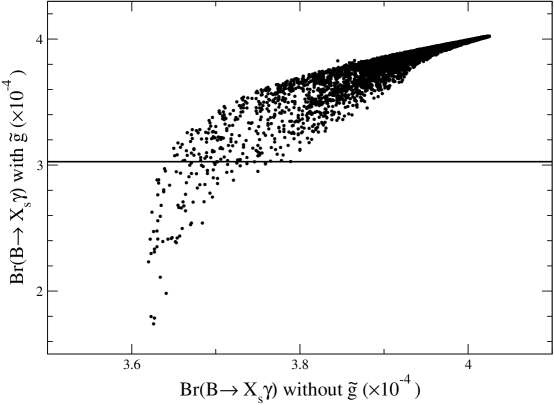
Figure 2: Plot of Br($\overline{B}\to X_{s}\gamma$) with and without the $\tilde{g}$ contributions. The horizontal line on the graph represents the $2\sigma$ experimental lower limit. These points all have $m_{H^{\pm}}=300\,{\rm GeV}$, $\mu=1\,{\rm TeV}$ and $\tan\beta=30$.

In order to create this plot we calculated the squark and gaugino spectra using the 1-loop renormalization group equations. The Higgs masses were determined using the highly precise calculation encoded into CPSuperH [15]. So that non-physical models, or models already ruled out experimentally, were not included among the points in the figure, we applied a set of cuts to the parameter space; specifically, we required that the lightest neutralino be the lightest SUSY particle (LSP), $m_{\tilde{t}_{1}}>96\,{\rm GeV}$, $m_{\tilde{\chi}^{\pm}_{1}}>103\,{\rm GeV}$ and $m_{h}>90GeV$.

The light Higgs mass bound is the most complicated. The bound for a SM-like Higgs is $114\,{\rm GeV}$ [16], but can be lower in extensions of the SM, especially those with additional light Higgs fields. We have examined our results from Figure 2 for tighter cuts on the Higgs mass, all the way up to $114\,{\rm GeV}$. We find that the points with the largest gluino contributions to $b\to s\gamma$ tend to have the lightest Higgs masses, and are therefore cut out of the parameter space as the Higgs mass constraint is tightened. The reason is simple: light Higgs masses well above the $Z$-mass require large top squark masses. But because of the mSUGRA boundary conditions, this drives the bottom squark masses to also be heavy, and these in turn force the gluino loops in $b\to s\gamma$ to decouple. One way to satisfy both requirements is, for example, to modify the mSUGRA boundary conditions so that the $\tilde{t}_{R}$ becomes heavy separately from the other squarks, which pushes up the Higgs mass without directly affecting the gluino loop in $b\to s\gamma$. We examined models in which $m_{\tilde{U},0}$ was varied independently of the other squark masses, and the effect of the Higgs mass constraint was essentially eliminated.

One last constraint applied to the points in the figure is that one or the other calculation of Br$(\overline{B}\to X_{s}\gamma)$ has so fall within the experimental 95% confidence region: $(3.03\div 4.07)\times 10^{-4}$. Points in which both calculations (with and without gluinos) fall outside that range are eliminated, but points in which one or the other calculation falls within the range are kept. This allows us to see quite clearly that the effect of the gluino contributions can be quite large, though its sign is always the same: the branching fraction with the gluinos included is always lower than that without the gluino. (We will discuss the reasons for this in detail below.) Thus the gluino contributions tend to rule out models which would otherwise appear to be consistent with experiment, tightening constraints in the parameter space.

In Figure 3 we have shown the same set of points in a different way, in order to emphasize the magnitude and sign of the gluino effect. Here we plot $\tan\beta$ versus the normalized difference in the two calculations of $\overline{B}\to X_{s}\gamma$. Specifically, we plot along the $y$-axis the quantity:

$$\delta\,\mbox{Br}_{\,b\to s\gamma} = \frac{\mbox{Br}(\overline{B}\to X_{s}\gamma)_{\rm no\,\,\tilde{g}}-\mbox{Br}(\overline{B}\to X_{s}\gamma)_{\rm with\,\,\tilde{g}}}{\mbox{Br}(\overline{B}\to X_{s}\gamma)_{\rm SM}},$$ (48)

normalized by the SM branching ratio given to be $3.15\times 10^{-4}$. The figure again shows the the decrease of the branching ratio due to the gluino contributions, but also the strong dependence on $\tan\beta$, which is expected since we require large $\tan\beta$ in order to generate significant LR mixing. We could also have plotted $|\mu|$ on the $x$-axis, but the shape would have been identical, since the LR mixing insertion is of the form $\mu\tan\beta$.

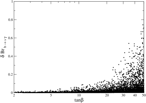
Figure 3: Plot of $\delta$Br$(\overline{B}\to X_{s}\gamma)$ vs. $\tan\beta$ normalized by the SM theoretical ratio of $3.15\times 10^{-4}$

Notice in the figure, again, that the gluino contributions always pull down the rate for $b\to s\gamma$ (and by as much as 50% in many cases). When $\mu$ is positive, the gluino diagrams have the opposite sign from the $W^{\pm}$ and $H^{\pm}$ diagrams, having the effect of partially canceling out the $H^{\pm}$ piece and pulling the branching ratio more in line with experiment. But since the sign of the gluino contribution is pegged to the sign of $\mu$, one should expect to see the opposite behavior for $\mu<0$. In fact, this is the case, though it cannot be seen from the figure. For $\mu<0$ and $\tan\beta$ large we find all points, with and without the gluinos included, to be above the experimental limit. Thus only the $\mu>0$ case is important for us, and so we always see it destructively interfere with the SM and charged Higgs contributions.

The first conclusion we should draw from these results is that is $\tan\beta$ happens to be large, then it is quite possible for gluino diagrams to contribute significantly to the rate for $b\to s\gamma$. This is true even in the models where one would least expect it, namely MFV models. This contribution is almost uniformly ignored in the literature and has the effect of ruling out models which might otherwise have been thought to be consistent with current experimental bounds.

Second, if the gluino contribution is non-negligible, then it should be possible to extract it from the data, which would in turn provide us with an avenue for measuring $(\Delta^{d}_{32})_{LL}$. Of course extracting the gluino contribution from the data requires a careful measurement of the physical masses and mixings that enter the MSSM calculation of $b\to s\gamma$. This will represent quite a challenge, since it requires the measurement of chargino and top squark mixing angles. The gluino contribution also requires as input the bottom squark mixing (in the guise of $(\Delta^{d}_{33})_{LR}$) if we hope to extract the 3-2 mixing angle. Nonetheless, once sufficient measurements of gaugino and squark masses and mixings have been made, the problem of extracting the inter-generational mixing will become important, because it will be one of the few tests we will have for the underlying flavor independence of the SUSY-breaking sector. In particular, having a set of tests (or even a single test) of the MFV scenario will be of great importance. Since the sum rules explicitly test minimal flavor violation, and do so in a way that is independent of the exact scale or nature of the mass unification, makes them a valuable tool for doing just that.

Finally, what of other tests of MFV other than $b\to s\gamma$? We have examined a number of other FCNC’s for sensitivity to minimal flavor violation and for usefulness of the sum rule approach. Though the sum rules can be quite good at extracting the mixings required to calculate gluino contributions to $K^{0}$-$\overline{K}^{0}$ and $B_{(s)}^{0}$-$\overline{B}_{(s)}^{0}$ mixing, we found the resulting contributions to be far too small to be interesting, at least in motivated models. There is also a well-known and large contribution of neutral Higgs bosons to $B_{(s)}^{0}$-$\overline{B}_{(s)}^{0}$ mixing [18], but at this time we can find no easy way to correlate those sources of flavor change to a set of sum rules. The best hope for extracting the new contributions to this process are by comparison to $B_{s}\to\mu\mu$ and $B\to X_{s}\mu\mu$ rates.

Conclusion

Though SUSY solves or alleviates a number of important problems within the structure of the Standard Model, it does so at a price. That price is the flavor problem, and it is this problem that has driven most of the model-building within the SUSY community for the last twenty years. With few exceptions (such as decoupling models), solutions to the flavor problem have generally fallen into the broad class of minimal flavor violation in which all quark flavor violation is tied to the Yukawa couplings.

In minimally flavor-violating models, there are still FCNCs, including those mediated by neutral particles such as neutralinos and gluinos. They are just suppressed by the unitarity of the CKM matrix and the near-degeneracy of the squarks. But the degeneracy is broken by the Yukawa couplings themselves, which re-introduces the FCNCs. Unfortunately the effects are small and difficult to extract directly from measurements at either the LHC or even some future linear collider. It is up to high-precision flavor experiments to measure the rates and processes that will allow extraction of the details of the SUSY flavor sector.

In this paper we derived a set of sum rules that can be used to extract the flavor mixing from the masses of the squark mass eigenstates, assuming minimal flavor violation. These sum rules provide a consistency check on minimal flavor violation. Even if the low-energy spectrum appears to be consistent with some kind of mass unification, the sum rules can be used to check this explicitly.

Finally, we showed that the classic FCNC decay $b\to s\gamma$ may be a particularly good place to look for these MFV contributions, via the gluino-mediated diagrams. Though the gluino contributions are often overlooked, at large $\tan\beta$ they may actually contribute enough to change the branching fraction by 50%. In such a case, it will be necessary to calculate the size of the $\tilde{s}_{L}$–$\tilde{b}_{L}$ flavor mixing, which is a job well-suited to the sum rules.

Once the mass spectrum of the MSSM is measured, assuming it is, it is questions about the flavor mixing that will ultimately help us disentangle the nature of the SUSY-breaking mechanism. Tools such as the sum rules, which connect flavor mixing to squark masses, could be key elements in this process.

References

[1]
S. Dimopoulos and D. W. Sutter,
Nucl. Phys. B 452, 496 (1995)
[arXiv:hep-ph/9504415].
[2]
G. D’Ambrosio, G. F. Giudice, G. Isidori and A. Strumia,
Nucl. Phys. B 645, 155 (2002)
[arXiv:hep-ph/0207036].
[3]
A. J. Buras,
Acta Phys. Polon. B 34, 5615 (2003)
[arXiv:hep-ph/0310208].
[4]
F. Gabbiani, E. Gabrielli, A. Masiero and L. Silvestrini,
Nucl. Phys. B 477, 321 (1996)
[arXiv:hep-ph/9604387].
[5]
F. Gabbiani and A. Masiero,
Nucl. Phys. B 322, 235 (1989).
[6]
S. Bertolini, F. Borzumati, A. Masiero and G. Ridolfi,
Nucl. Phys. B 353, 591 (1991).
[7]
S. P. Martin and P. Ramond,
Phys. Rev. D 48, 5365 (1993)
[arXiv:hep-ph/9306314].
[8]
S. P. Martin and M. T. Vaughn,
Phys. Rev. D 50, 2282 (1994)
[arXiv:hep-ph/9311340].
[9]
R. Barbieri and G. F. Giudice,
Phys. Lett. B 309, 86 (1993)
[arXiv:hep-ph/9303270].
[10]
W. Porod,
Comput. Phys. Commun. 153, 275 (2003)
[arXiv:hep-ph/0301101].
[11]
M. S. Carena, D. Garcia, U. Nierste and C. E. M. Wagner,
Phys. Lett. B 499, 141 (2001)
[arXiv:hep-ph/0010003].
[12]
T. Hurth, E. Lunghi and W. Porod,
Nucl. Phys. B 704, 56 (2005)
[arXiv:hep-ph/0312260].
[13]
M. Misiak et al.,
Phys. Rev. Lett. 98, 022002 (2007)
[arXiv:hep-ph/0609232].
[14]
F. Domingo and U. Ellwanger,
JHEP 0712, 090 (2007)
[arXiv:0710.3714 [hep-ph]].
[15]
J. S. Lee, A. Pilaftsis, M. S. Carena, S. Y. Choi, M. Drees, J. R. Ellis and C. E. M. Wagner,
Comput. Phys. Commun. 156, 283 (2004)
[arXiv:hep-ph/0307377].
[16]
R. Barate et al. [LEP Working Group for Higgs boson searches],
Phys. Lett. B 565, 61 (2003)
[arXiv:hep-ex/0306033].
[17]
E. Barberio et al. [Heavy Flavor Averaging Group (HFAG)],
arXiv:hep-ex/0603003.
[18]
A. J. Buras, P. H. Chankowski, J. Rosiek and L. Slawianowska,
Phys. Lett. B 546, 96 (2002)
[arXiv:hep-ph/0207241] and
Nucl. Phys. B 659, 3 (2003)
[arXiv:hep-ph/0210145].