Dispersion enhancement and damping by buoyancy driven flows in 2D networks of capillaries

Abstract

The influence of a small relative density difference ($\simeq 3.10^{-4}$) on the displacement of two miscible liquids is studied experimentally in transparent $2D$ networks of micro channels with a mean width $a$ held vertically. Maps of the local relative concentration are obtained by an optical light absorption technique. Both stable displacements in which the denser fluid enters at the bottom of the cell and displaces the lighter one and unstable displacements in which the lighter fluid is injected at the bottom and displaces the denser one are realized. Except at the lowest mean flow velocity U, the average $C(x,t)$ of the relative concentration satisfies a convection-dispersion equation. The relative magnitude of $|U|$ and of the velocity $U_{g}$ of buoyancy driven fluid motions is characterized by the gravity number $N_{g}=U_{g}/|U|$. At low gravity numbers $|N_{g}|<0.01$ (or equivalently high Péclet numbers $Pe=Ua/D_{m}>500$), the dispersivities $l_{d}$ in the stable and unstable configurations are similar with $l_{d}\,\propto Pe^{0.5}$. At low velocities ($|N_{g}|>0.01$), $l_{d}$ increases like $1/Pe$ in the unstable configuration ($N_{g}<0$) while it becomes constant and close to the length of individual channels in the stable case ($N_{g}>0$). Iso concentration lines $c(x,y,t)=0.5$ are globally flat in the stable configuration while, in the unstable case, they display spikes and troughs with an rms amplitude $\sigma_{f}$ parallel to the flow. For $N_{g}>-0.2$ $\sigma_{f}$ increases initially with the distance and reaches a constant limit while it keeps increasing for $N_{g}<-0.2$. A model taking into account buoyancy forces driving the instability and the transverse exchange of tracer between rising fingers and the surrounding fluid is suggested and its applicability to previous results obtained in $3D$ media is discussed.

I Introduction

Miscible displacements in porous media are encountered in many environmental, water supply and industrial problems bear72 ; dullien91 ; sahimi95 . Specific types of miscible displacements, like tracer dispersion, are also usable as diagnostic tools to investigate porous media heterogeneities at the laboratory charlaix88 or field scales. The characteristics of these processes, such as the width and the geometry of the displacement front, are often influenced by contrasts between the properties of the displacing and displaced fluids such as their density freytes01 ; oltean04 ; menand05 ; flowers2007 . In unstable density contrast configurations (fluid density increasing with height), gravity driven instabilities may appear and broaden the displacement front: as an unwanted result, this may lead to early breakthroughs of the displacing fluid. An example of such effects is the infiltration of a dense plume of pollutant into a saturated medium.

The objective of the present paper is to study experimentally at both the local and global scales miscible displacements of two fluids of slightly different densities ($\Delta\rho/\rho\simeq 3\times 10^{-4}$): of particular interest is the influence of buoyancy driven flow perturbations on the structure and development of the mixing zone.

In porous media, the characteristic velocity (counted positively for upwards flow) of buoyancy driven flow components is:

$$U_{g}=-k\frac{\Delta\rho g}{\mu}$$ (1)

in which $\Delta\rho$ is the density of the lower fluid minus that of the upper one, $\mu$ their viscosity and $k$ the permeability of the medium. The velocity $U_{g}$ is the estimation, from Darcy’s law, of the flow per unit area induced by the difference of the hydrostatic pressure gradients in the two fluids. The relative magnitude of $U_{g}$ and of the mean flow velocity $U$ is a key element in the present problem; it will be characterized by the gravity number flowers2007 :

$$N_{g}=-\frac{U_{g}}{|U|}=\frac{\Delta\rho gk}{\mu|U|}$$ (2)

With the above definition of $\Delta\rho$, one has $N_{g}>0$ in the stable configuration (denser fluid below the lighter one) and $N_{g}<0$ in the unstable one.

Recent experiments freytes01 ; oltean04 ; menand05 have shown that, even when the parameter $N_{g}$ is quite small, the geometry of the mixing fronts may still be strongly influenced by buoyancy. Variable density flow and transport in porous media has therefore received an increasing attention, in particular through theoretical and numerical investigations schincariol97 ; beinhorn05 ; johannsen06 .

In the present work, optical measurements of miscible displacements of fluids of slightly different densities are performed in a transparent two-dimensional vertical network of channels with random widths zarcone83 . The experiments combine visualizations at the pore scale (one of the fluids is dyed) and measurements of the global concentration profiles parallel to the mean flow at different mean velocities $U$. Comparing displacement processes in stable and unstable density contrast configurations allows one to detect and characterize the development and influence of buoyancy driven flows.

Here, the density contrasts are low enough so that the $|N_{g}|$ remains small; under such conditions the hydrodynamic dispersion damps the development of instabilities. Then the mixing process can be considered as dispersive and is well described by the macroscopic convection-dispersion equation classically used for passive tracers with:

$$\frac{\partial C}{\partial t}=\vec{\nabla}.(\vec{U}.C-\bar{D}.\vec{\nabla}C),$$ (3)

where $C$ is the tracer concentration, $\vec{U}$ the flow velocity and $\bar{D}$ the dispersion tensor (all values are averaged over the gap of the cell); $\bar{D}$ is assumed to reduce to the diagonal components $D_{\parallel}$ and $D_{\perp}$ corresponding to directions respectively parallel and perpendicular to the mean flow. The values of $D_{\parallel}$ and $D_{\perp}$ are determined by two main physical mechanisms: advection by the velocity field inside the medium and molecular diffusion (characterized by a molecular diffusion coefficient $D_{m}$). The relative magnitude of these two effects is characterized by the Péclet number $Pe=Ua/D_{m}$ ($a$ is here the average channel width).

Both immiscible displacements zarcone83 and tracer dispersion charlaix88 ; dangelo07 have already been measured previously in such models. This latter work dangelo07 uses the same experimental technique and porous model as the present one but deals with experimental conditions in which the development of buoyancy driven instabilities is negligible. In this case, the dye can be considered as an “ideal” tracer that does not modify the fluid properties. In contrast, the present work deals with the influence of buoyancy effects on dispersion: the components of $\bar{D}$ depend on $\Delta\rho$ and are larger in the unstable configuratio. Similar studies might be performed on $3D$ porous samples using NMR-Imaging, CAT-Scan, acoustical techniques wong99 ; kretz03 or Positron Emission Projection Imaging tenchine05 but at a higher cost and/or with strong constraints on the fluid pairs to be used.

In the present displacement experiments, concentration maps obtained for a vertical flow are compared for different flow velocities and fluid rheologies. At the global scale, an effective dispersion coefficient is determined and its dependence on the flow velocity is studied in both stable and unstable density contrast configurations. At the local scale, the variation of geometrical front features of different sizes is analyzed as a function of the flow velocity and of time. The combination of these local and global data provides both a sensitive detection of the instabilities and information on the characteristics of the displacement process at different length scales. The $2D$ models of porous media used here are characterized by a random spatial distribution of the local permeability: the development of the front geometry under the combined action of these permeability variations and of destabilizing density contrasts is of particular interest.

II Description of experiment

II.1 Experimental setup and procedure

The experimental system and the technique for analyzing the data have already been described in reference dangelo07 . The model medium is a vertical transparent two dimensional square network of channels of random aperture zarcone83 : it has a mesh size equal to $d=1\,\mathrm{mm}$ and contains $140\times 140$ channels with a mean length $0.67\,\mathrm{mm}$ and a depth $0.5\,\mathrm{mm}$. The width of the channels takes $7$ values between $0.1$ and $0.6\,\mathrm{mm}$ with a log-normal distribution and a mean value $a=0.33\,\mathrm{mm}$. The permeability of the network is $k=3.10^{-9}\,\mathrm{m}^{2}$ (i.e. $3000$ Darcy).

The model is vertical with its open sides horizontal (see Figure 2 in reference dangelo07 ). Its upper side is connected to a syringe pump sucking the fluids upward out of the model from a reservoir inside which the lower side is dipped. Initially, the model is saturated by pumping the first fluid of density $\rho_{1}$ out of the lower reservoir into the model. Then, the pump is switched off and the lower side of the model is removed from the liquid bath by lowering the reservoir (the connection tubes are shut to avoid unwanted fluid exchange between the model and the outside during this process). The reservoir is then emptied completely, filled up by the second fluid of density $\rho_{2}=\rho_{1}+\Delta\rho$ and raised again until the lower side of the model is below the liquid surface. The displacement process is initiated by opening the connection tubes and switching on the pump. This procedure provides a perfectly straight initial front between the two fluids at the beginning of the displacement.

In this work, the absolute value $|\Delta\rho|$ of the density difference between the two fluids is constant with $|\Delta\rho|=0.3\,\mathrm{kg/m}^{3}$. For each flow rate and pair of fluids used, both stable ($\Delta\rho>\ 0$) and unstable ($\Delta\rho<\ 0$) configurations are studied by swapping fluids $1$ and $2$.

II.2 Fluid characteristics

Newtonian water-glycerol mixtures or shear thinning water-polymer solutions are used in the experiments. The mean flow velocity ranges from $0.005$ to $2.5\,\mathrm{mm.s}^{-1}$. The injected and displaced fluids are identical but for Water Blue dye added to one of the solutions, allowing one to both measure the local concentration optically and to introduce a controllable density difference between the fluids (note that, since the density contrast is purely due to the dye, the optical determination of the local dye concentration also measures the local density which is proportional to this concentration). The molecular diffusion coefficient $D_{m}=6.5\,\times 10^{-4}\,\mathrm{mm}^{2}\mathrm{.s}^{-1}$ of the dye is practically the same in the polymer solutions as in pure water.

The Newtonian water-glycerol solution used is obtained by mixing $60\%$ in weight of glycerol in pure water. Its viscosity is equal to $\mu=10^{-2}\,\mathrm{Pa.s}$ at $20\,^{o}\mathrm{C}$ so that the molecular diffusion coefficient (proportional to $\mu^{-1}$) is $D_{m}^{*}=0.7\times 10^{-4}\,\mathrm{mm}^{2}\mathrm{.s}^{-1}$.

The shear thinning solutions have concentrations $C_{p}=500$ and $1000\,\mathrm{ppm}$ of high molecular weight Scleroglucan (Sanofi Bioindustries) in water. The variation of their effective viscosity $\mu$ with the shear rate $\dot{\gamma}$ (see Figure 1 of ref. dangelo07 ) are well adjusted by the Carreau function:

$$\mu=\frac{1}{(1+(\dot{\gamma}/\dot{\gamma_{0}})^{2})^{\frac{1-n}{2}}}(\mu_{0}-\mu_{\infty})+\mu_{\infty}.$$ (4)

The values of these rheological parameters for the solutions used in the present work are listed in Table 1. The limiting value $\mu_{\infty}$ cannot be measured directly and is taken equal to the viscosity of the solvent, i.e. water, namely: $\mu_{\infty}\,=\,10^{-3}\,\mathrm{Pa.s}$. In Eq. (4), $\dot{\gamma_{0}}$ corresponds to the transition between a “Newtonian plateau” domain at low shear rates ($\dot{\gamma}<\dot{\gamma_{0}}$) in which $\mu=\mu_{0}$ and a domain in which $\mu$ decreases with $\dot{\gamma}$ following the power law $\mu\propto{\dot{\gamma}}^{(n-1)}$ ($\dot{\gamma}>\dot{\gamma_{0}}$).

$C_{p}$	$n$	$\dot{\gamma_{0}}$	${\mu}_{0}$	$U^{*}$
ppm		$\mathrm{s}^{-1}$	$\mathrm{mPa.s}$	$\mathrm{mm.s}^{-1}$
$500$	$0.38\pm 0.04$	$0.077\pm 0.018$	$410\pm 33$	$0.045$
$1000$	$0.26\pm 0.02$	$0.026\pm 0.004$	$4500\pm 340$	$0.013$

Table 1: Rheological parameters of scleroglucan solutions used in the flow experiments. $C_{p}$ refers to the polymer concentration in ppm. The transition mean velocity $U^{*}$ is estimated by assuming a velocity gradient equal to $\dot{\gamma_{0}}$ at the walls of a channel of width $a$ with a parabolic velocity profile.

The model is illuminated from the back by a fluorescent light panel and images are acquired by a $12$ bits high stability digital camera with a $1030\times 1300$ pixels resolution (pixel size = $0.16\,\mathrm{mm}$). Typically, $100$ images are recorded for each experimental run at time intervals between $2.5$ and $700\,\mathrm{s}$. The images are then translated into maps of the relative concentration $C(x,y,t)$ of the two fluids in the model using a calibration procedure already described in refs. dangelo07 ; boschan07 and commonly used menand05 .

II.3 Characteristic parameters of buoyancy driven flows

For the water-glycerol mixture, all parameters are fixed and the modulus $|U_{g}|$ of the buoyant flow velocity (see Eq.(1)) is constant (only its sign changes when the fluids are swapped): the gravity number $N_{g}$ varies then as $U^{-1}$ with the velocity and the influence of gravity is largest at the lowest velocities.

For polymer solutions, the effective viscosity varies with the shear rate following Eq. (4). and the value of $N_{g}$ can only be computed at low flow velocities $U<U^{*}$ for which the shear rate $\dot{\gamma}$ is lower than $\dot{\gamma_{0}}$ in the whole model and $\mu=\mu_{0}=cst.$ so that $N_{g}$ varies again as $U^{-1}$. At velocities $U>U^{*}$ such that the shear rate is larger than $\dot{\gamma_{0}}$ in some parts of the model, the viscosity $\mu$ varies spatially and $N_{g}$ cannot be computed simply. However, at high shear rates one has: $\mu\propto dot{\gamma}^{n-1}$. Since $N_{g}\propto 1/(\mu|U|)$, its effective value will be proportional to $\dot{\gamma}^{-n}$: although its actual value cannot be computed, $N_{g}$ also decreases when $U$ increases in this shear thinning regime. Due to this globally monotonous variation, the first instabilities will still appear at the lowest velocities and, often, in the Newtonian domain where $\mu=\mu_{0}$ so that $U_{g}=-\Delta\rho gk/\mu_{0}$.

The velocity $U_{g}$ has been estimated for the fluids used in the present work, leading to $|U_{g}|=10^{-3},\ 2.10^{-5}$ and $2.10^{-6}\,\mathrm{mm.s}^{-1}$ for respectively the glycerol-water mixture and the $500\,\mathrm{ppm}$ and $1000\,\mathrm{ppm}$ polymer solutions (assuming $\mu=\mu_{0}$). At the lowest experimental flow velocity ($U=5.10^{-3}\,\mathrm{mm.s}^{-1}$), the duration of the complete saturation of the network is $t\simeq 3.10^{4}\,\mathrm{s}$. During this time lapse, the distance $U_{g}.t$ characterizing the growth of the gravitational instabilities is $28\,\mathrm{mm}$ for the water glycerol mixture: this is far above the length $d$ of the individual channels of the network and a noticeable influence of gravity on the structure of the displacement fronts is thus expected. For the polymer solutions, this same distance is less than $0.6\,\mathrm{mm}$, i.e. smaller than $d$; the dye should behave therefore in this case like an ”ideal” tracer.

For water-glycerol solutions, buoyancy effects should be sizable when the distance $U_{g}~{}t$ becomes larger than $d$: the transition should then take place at an imposed flow velocity $U_{c}=U_{g}.L/d\simeq 0.14\ mm.s^{-1}$ ($L$ is the network length). This velocity correspond to the following gravity and Péclet numbers : $N_{g}^{c}\simeq 0.01$ and $Pe^{c}\simeq 500$. These predictions will be shown In Section III.3 to correspond well to the experimental results.

III Experimental results

III.1 Qualitative observations of miscible displacements

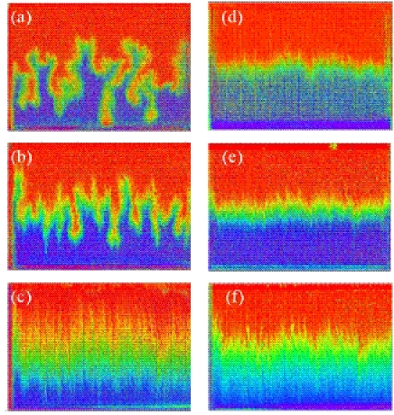
Figure 1: Relative concentration maps for experiments using water-glycerol solutions of different densities at three different flow rates: (a, d) $U=0.005\,\mathrm{mm.s}^{-1}$ - $|N_{g}|=0.2$; (b, e) $U=0.025\,\mathrm{mm.s}^{-1}$ - $|N_{g}|=0.04$ and (c,f): $U=1.25\,\mathrm{mm.s}^{-1}$ - $|N_{g}|=8.10^{-4}$. Experiments correspond to stable (d, e, f) and unstable (a, b, c) density contrast configurations at a time when the injected fluid occupies roughly half of the model. In these figures and in the following ones, darker shades correspond to the pure injected or displaced fluid and the lighter shade to a mixture of the two. Fluid flows are upwards with $\vec{g}$ pointing downwards. The field of view of the pictures is $153\mathrm{mm}\times 140\mathrm{mm}$.

Figure 1 displays concentration distributions observed during displacement experiments using the water-glycerol mixture. In the stable configuration of Figures 1 d,e and f, the mean global front shape remains flat at all flow velocities. The overall width of the mixing zone increases however with the flow rate due to the development of fine structures parallel to the mean flow, particularly at the highest velocity (Fig. 1f).

In the unstable configuration, and at the lowest velocity (Fig. 1a), large instability fingers with a width of the order of $10$ to $15$ mesh sizes appear and grow up to a length equal to that of the experimental model. For a velocity four times higher, fingers still appear but they are significantly shorter (Fig. 1b). As the velocity increases, the size of the fingers parallel to the mean flow decreases while finer features develop. For a velocity still $50$ times higher (Fig. 1c), the front geometry is more similar to that observed in the stable case although its width parallel to the flow is still broader. In section III.4, the structure of the mixing zone in these experiments will be analyzed again in the unstable case from the geometry of the iso-concentration fronts ($C(x,y,t)=0.5$).

Similar pictures from experiments realized with a $C_{p}=1000\,\mathrm{ppm}$ water-scleroglucan solution are displayed in Figure 2. In contrast with the case of the water-glycerol solutions, no buoyancy induced instability appears in the unstable configurations (cases a,b), even at low velocities (a) and the relative concentration maps in both configurations are very similar. At high velocities, fine structures similar to those observed for the Newtonian solution appear on the front (cases a,c). Finally, comparisons of front geometries observed for $C_{p}=500$ and $1000\,\mathrm{ppm}$ and displayed in Figure 3 of ref. dangelo07 show that intermediate scale structures of the front (with a width of 10-20 mesh sizes) appear at the same locations for both concentrations.

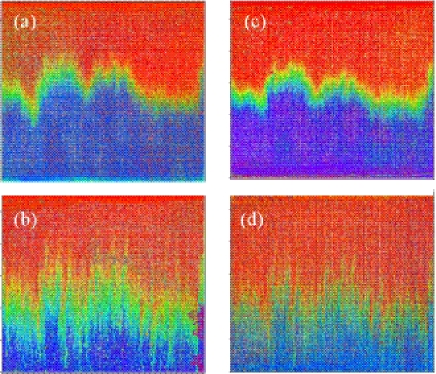
Figure 2: Relative concentration maps for experiments using $1000\,\mathrm{ppm}$ water-scleroglucan solution in gravitationally unstable (a,b) resp. stable (c,d) configurations for several flow velocities and gravity number values : $U=0.005\ mm.s^{-1}$ - $|N_{g}|=4.10^{-4}$ (a,c) and $U=0.5\ mm.s^{-1}$ - $|N_{g}|=4.10^{-6}$ (b,d). Grey scale codes and flow direction are the same as in Figure 1 and the field of view is also identical.

Globally, the above results are in qualitative agreement with macroscopic dispersion measurements realized on three-dimensional bead packs freytes01 using conductivity tracers detected at the outlet of the samples. In these experiments, buoyancy driven instabilities are also observed at low velocities for Newtonian water-glycerol solutions in a gravitationally unstable configuration but do not appear for water-scleroglucan solutions. Compared to this latter work, the optical measurements provide additional information on the dependence of the front structures of different sizes on the control parameters. We examine now the variation of the global dispersion characteristics as a function of the experimental parameters and of the configuration of the fluids.

III.2 Quantitative concentration variation analysis

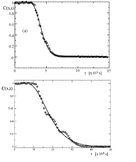
Figure 3: Normalized mean concentration variation $C(x,t)$ as a function of the time $t$ for unstable displacement experiments using a water glycerol mixture ($C$: average of local pixel concentration $c(x,y,t)$ over a width $\Delta y\simeq 144\,\mathrm{mm}$ in the central part of the model). (a) $U=0.025\,\mathrm{mm.s}^{-1}$, $N_{g}=-0.04$, $x=104\,\mathrm{mm}$. - (b) $U=0.005\,\mathrm{mm.s}^{-1}$, $N_{g}=-0.2$, $x=88\,\mathrm{mm}$. Continuous line: fit by a solution of Equation (3) with (a) $\overline{t}=4350\,\mathrm{s}$, $D_{\parallel}/U^{2}=110\,\mathrm{s}$ and (b) $\overline{t}=18266\,\mathrm{s}$, $D_{\parallel}/U^{2}=1369\,\mathrm{s}$

. The determination of the mean velocity $U$ is discussed below in the present section III.2.

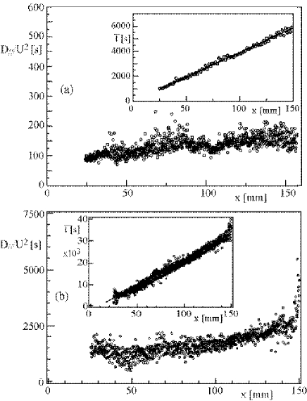
Figure 4: Variation of the fitting parameter $D_{\parallel}/U^{2}$ as a function of the distance $x$ from the inlet for two unstable displacement experiments using the water glycerol solutions with $U=0.025\,\mathrm{mm.s}^{-1}$ ($N_{g}=-0.04$) and $U=0.005\,\mathrm{mm.s}^{-1}$ ($N_{g}=-0.2$). Insets: variation of the mean transit time $\overline{t}$ as a function of $x$. Solid line: linear regression of the data. Values of $\overline{t}$ and $D_{\parallel}/U^{2}$ are obtained by fitting the mean concentration variation $C(x,t)$ using Eq. (3) at each distance $x$.

The procedure for determining a global dispersion coefficient from the concentration maps is described in detail in reference dangelo07 . The mean relative concentration $C(x,t)$ of heavy (dyed) fluid at a distance $x$ from the inlet side is first determined by averaging the value $c(x,y,t)$ for individual pixels over a window of width $\Delta y=144\ mm$ representing almost the full width of the model across the flow (only pixels located inside the pore volume are included in the average). More local information is obtained from the geometry of iso-concentration curves and will be discussed below.

Figures 3a-b display the variations with time of $C(x,t)$ for two different values of the gravity number $N_{g}$. These variations have been fitted (continuous line) by the following one dimensional-solution of the convection diffusion equation (3) (assuming a concentration $C$ constant with y, an initial step-like variation of $C$ at the inlet and taking $D_{\parallel}$ equal to the diagonal component of the tensor $D$ in the $x$ direction) :

$$C(x,t)=\frac{1}{2}\left[1-\frac{N_{g}}{|N_{g}|}.\,erf\left(\frac{t-{\overline{t}}}{\sqrt{4D_{\parallel}t/U^{2}}}\right)\right]$$ (5)

Since flow is always upwards, adding the factor $N_{g}/|N_{g}|=\pm 1$ makes the equation usable both for light fluid displacing heavy fluid (unstable configuration - $N_{g}<0$) and heavy fluid displacing light fluid (stable configuration - $N_{g}>0$).

For $N_{g}=-0.04$, one observes a good fit of the experimental data with Eq. (5). For $N_{g}=-0.2$ for which the distortions of the front due to the instabilities are very large, the concentration does not decrease smoothly but the experimental curve displays bumps; these features are the signature of rising fingers reaching the measurement height. Yet, an acceptable fit of the experimental data with Eq. (5) can still be achieved. The fits provide the values of the mean transit time $\overline{t}$ of the front at the distance $x$ and of the ratio $D_{\parallel}/U^{2}=\bar{\Delta}t^{2}/(2\overline{t})$ ($\bar{\Delta}t^{2}$ is the centered second moment of the transit times along the distance $x$).

The insets of figures 5a-b display the variation of $\overline{t}$ with the distance $x$ which is linear in both cases; this shows that the mixing zone characterized by the mean concentration profile $C(x,t)$ moves at a constant velocity $U_{mz}$ which is equal to the inverse of the slope of the variation. A linear regression of the data provides the values $U_{mz}=0.027\ \mathrm{mm.s}^{-1}$ for case $(a)$ and $U_{mz}=0.0046\ \mathrm{mm.s}^{-1}$ for $(b)$. The mean fluid velocity $U$ in the model may be taken equal to the ratio of the injected flow rate and of the pore volume per unit length along $x$ which have been determined independently. The values of $U$ computed in this way at the same two flow rates as above are respectively $U=0.025$ and $0.005\mathrm{mm.s}^{-1}$: they are very close to the corresponding values of $U_{mz}$.

The two velocities $U$ and $U_{mz}$ are compared more precisely in Figure 6 which displays the values of $U_{mz}/U$ for both stable ($\circ$) and unstable ($\bullet$) flow configurations,. This ratio is always close to $1$: this shows that buoyancy effects do not influence the mean displacement of the concentration profile, even at the lowest flow rate ($N_{g}=-0.2$) for which they are very large (Fig.2a). One assumes therefore in the following that $U=U_{mz}$.

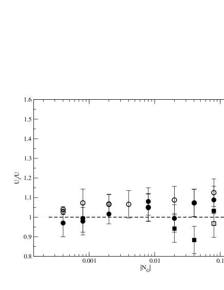
Figure 5: Variation as a function of $|N_{g}|$ of the characteristic velocities of the fluid displacement normalized by the mean velocity $U$ in stable (open symbols) and unstable (dark symbols) density contrast configurations. ($\circ$),($\bullet$): normalized velocity of the mixing region $U_{mz}/U$ determined by a linear regression on the variation of $\overline{t}$ as a function of $x$ (see insets of Fig. 4a-b). ($\square$, $\blacksquare$) $U_{c0.5}$ = mean velocity of iso-concentration lines $c=0.5$.

The main graphics of Figures 4(a-b) display the variation of the ratio $D_{\parallel}/U^{2}$ as function of the distance $x$ from the inlet. In case (a) ($N_{g}=-0.04$), $D_{\parallel}/U^{2}$ increases at first slightly with the distance $x$ and levels off for $x\geq 50\ mm$; then, it fluctuates around a constant value. Previous studies dangelo07 have shown that the fluctuations are periodic and determined by the structure of the network (the period is equal to the mesh size). In case (b) ($N_{g}=-0.2$), $D_{\parallel}/U^{2}$ fluctuates around a constant value for $x\leq 100\,\mathrm{mm}$. At larger distances, a slight steady increase of $D_{\parallel}/U^{2}$ with $x$ is observed. This is likely due to the rising fingers, directly observable in Fig.1a and which can be identified on the curve of Fig.3b. Tracers are advected faster and farther inside these fingers than outside, resulting in an increase of the dispersivity. Even in this case, however, the fluctuations of the measurements and the relatively small variations of the values of $D_{\parallel}/U^{2}$ do not allow one to conclude that a diffusive regime is not reached.

These results show both that the mixing front moves at a constant velocity $U$ and that (except perhaps for $N_{g}=-0.2$) it reaches a dispersive spreading regime characterized by a dispersion coefficient $<D_{\parallel}>$ taken equal to the average of $D_{\parallel}$ over the full experimental range of $x$ values. In the following, like in ref. dangelo07 , the dispersivity $l_{d}\ =\ <D_{\parallel}>/U$ is generally used instead of $<D_{\parallel}>$ to characterize the dispersion process. Finally, the standard deviation of the individual values of $D_{\parallel}$ will be used to estimate the error bars on $l_{d}$.

III.3 Global dispersion measurement results

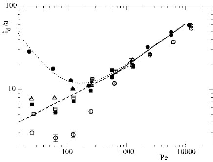
Figure 6: Variation of the dispersivity $l_{d}/a=D/aU$, as a function of the Péclet number $Pe$ for different fluids. $(\circ,\ \bullet)$: water-glycerol mixture; $(\square,\ \blacksquare)$: $500$ ppm and $(\triangle,\blacktriangle)$: $1000$ ppm polymer solutions. Light symbols: $N_{g}<0$; dark symbols: $N_{g}>0$. Upper axis: values of $|N_{g}|$ for the Newtonian water-glycerol solutions. Dashed line: variation law $l_{d}/a=1.5\,Pe^{0.35}$ satisfied from ref. dangelo07 by data corresponding to the polymer solution. Solid ($l_{d}/a=0.6\,Pe^{0.5}$) and dash-dotted ($l_{d}/a=0.5\,Pe^{0.5}$) lines:, regression for water-glycerol data respectively for the unstable and stable configurations in the buoyancy free flow domain ($|N_{g}|<N_{g}^{c}=0.01$). Dotted line: variation predicted by Eq. (10) based on the model described in section IV below (the dispersivity is assumed to be the sum of a passive tracer component and of a buoyancy term which decreasing with $Pe$). The fitting parameters are $\beta_{T}=0$ and $\epsilon=0.3$.

In the present section, we discuss the variations of the normalized dispersivity $l_{d}/a$ as a function of the flow velocity in the stable and unstable configurations: these variations are displayed in Figure 6 for the different solutions investigated (the horizontal scales are the Péclet number $Pe=Ua/D_{m}$ (bottom axis) and the gravity number $|N_{g}|$ (top axis).

For water-glycerol solutions, there is a clear separation at high $N_{g}$ (or equivalently low Pe) values between data points corresponding to unstable ($N_{g}<0$) and stable ($N_{g}>0$) density contrast configurations: this separation occurs occurs close to the transition value $N_{g}^{c}=0.01$ (respectively $Pe^{c}=500$) discussed in Sec. II.3. Such a separation has also been previously reported in 3D bead packings freytes01 : in Sec. IV, these $3D$ observations will be compared quantitatively to the present $2D$ measurements. This separation reflects the development of finger like structures at low velocities in the unstable configuration ($N_{g}<0$) and the flattening of the front in the stable one ($N_{g}>0$). These features are due to buoyancy forces and are qualitatively visible in Figure 6. At the lowest Péclet number, the values of $l_{d}$ for $N_{g}>0$ and $N_{g}<0$ differ by a factor of nearly $10$.

For $N_{g}>0$, the dispersivity $l_{d}$ reaches for $N_{g}\simeq 2\times 10^{-3}$ ($Pe\simeq 100$) a low minimum value $l_{d}\simeq 1\,\mathrm{mm}$ close to the characteristic local length, i.e. the mesh size of the lattice. In most usual homogeneous porous media, and in the case of a perfectly passive tracer, this latter value represents a lower limit of $l_{d}$: finding such a low value here confirms the stabilizing influence of the buoyancy forces flowers2007 .

For displacements of water-polymer solutions in the same range of $Pe$ values, the variations of $l_{d}$ with $Pe$ are the same for the stable and unstable flow configurations: this result was qualitatively visible in Figure 2 for the $1000\,\mathrm{ppm}$ solution and is confirmed quantitatively in Figure 6 for both polymer concentrations. This implies that no fingering instabilities develop in the unstable case and that the front is not flattened by gravity in the stable one.

Quantitatively, from Sec. II.3, an upper limit of the value of $N_{g}$ can be estimated by taking $\mu=\mu_{0}$ in Eq. (2) at the lowest experimental flow velocity. This gives: $|N_{g}|=5\times 10^{-3}$ and $|N_{g}|=4.5\times 10^{-4}$ respectively for the $500$ and $1000\,\mathrm{ppm}$ solutions, i.e. below the threshold of the instabilities observed for the Newtonian fluids. Since, $N_{g}$ decreases at higher flow velocities, this confirms that no effect of buoyancy will be observable in the experimental range of velocities (in agreement with the experimental observations and with the discussion of Sec. II.3).

At high velocities ($U>0.1\,\mathrm{mm.s}^{-1}$ (or $Pe>500$ for water-glycerol and $Pe>50$ for the polymer solutions), $l_{d}$ takes similar values for both $N_{g}>0$ and $<0$ and increases with $Pe$ as $l_{d}\propto Pe^{\alpha}$ with $\alpha=0.5$ at high $Pe$ values in both the unstable and stable configurations (solid and dash dotted lines in Figure 6). A similar behaviour has aleady been reported ref. dangelo07 for water polymer solutions but with a lower exponent $\alpha=0.35$: the variation differs in both cases from the slow increase observed in three-dimensional media such as an homogeneous monodisperse grain packing freytes01 . The $Pe^{\alpha}$ variation reflects the combined effects of geometrical dispersion due to the disorder of the velocity field and of Taylor dispersion due to the velocity profiles in individual channels. The latter becomes important at high Péclet numbers due to the reduced mixing at the junctions by transverse molecular diffusion. As a result, the correlation length of the velocity of the tracer particles along their trajectories (and, therefore, the dispersivity $l_{d}$) become larger. The difference between the values of $\alpha$ for the Newtonian and shear thinning solutions is likely due to the different relative weight of the two mechanisms in the two cases: as discussed in refs. dangelo07 ; boschan07 , Taylor dispersion is indeed reduced and geometrical dispersion is enhanced for shear thinning fluids compared to the Newtonian case.

The above analysis of the global dispersion discussed above uses averages of the local concentration over nearly the full width of the model and encompassing therefore all the geometrical features of the front instabilities. The corresponding global value of $l_{d}$ combines then different types of effects.

A first one is the local spreading of the displacement front. It is likely to result from the combined effects the local disorder of the flow field (geometrical dispersion mechanism) and the flow profile between the rough walls (Taylor mechanisms). The effect of these mechanisms in the present system is discussed in ref. dangelo07

A second, more global, effect is the global spreading of the mixing zone due to the fluid velocity contrasts between different flow paths (associated, for instance, to the development of the instabilities). This is studied now specifically from the variations of the front geometry.

III.4 Spatial structure of the displacement fronts for unstable flows

Previous experiments in three dimensional porous media kretz03 demonstrated a clear amplification of front structures resulting from permeability heterogeneities for unstable density contrast configurations. Such effects can be studied precisely here down to small lengths scales thanks to the two-dimensional geometry of the model network and to the high precision and spatial resolution of the optical concentration measurements.

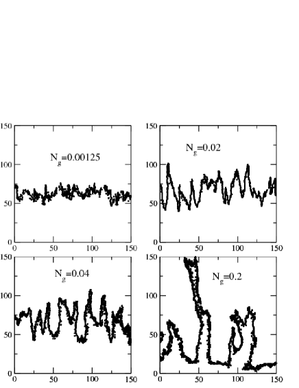
Figure 7: Iso concentration fronts $x_{f}(y,t)$ measured at four different gravity numbers $N_{g}=-0.00125$ (a), $-0.02$ (b), $-0.04$ (c) and $-0.2$ (d) for water-glycerol mixtures in an unstable flow configuration (the injected fluid occupies half of the model area). Flow is upwards with $\vec{g}$ oriented downwards. The inset in figure $b$, displays the typical size of the spikes $\lambda$.

In the following, the front geometry is characterized from the lines $x_{f}(y,t)$ along which the local relative concentration $c(x,y,t)$ is equal to $0.5$ at a given time $t$. Examples of such lines determined by a thresholding procedure at four gravity numbers $-0.001\geq N_{g}\geq-0.2$ are displayed in Fig. 7.

At the lowest flow velocity investigated ($N_{g}=-0.2$, $Pe\simeq 25$), the buoyancy driven flow components have a major influence on the front geometry and several instability fingers soar up while the front displacement is much slower in other regions (Fig. 7d).

At higher mean flow velocities (Fig. 7b-c) the front retains a rough geometry, still reflecting buoyancy driven flow components but its mean advancing motion is clearly visible. In contrast, for $N_{g}=-0.2$ (Fig. 7d), the development of the front appears as the combination of the independent growth of the individual fingers.

Another important feature is the fact that the distance $y$ across the front at which corresponding geometrical features (peaks and troughs) appear remains the same. For $N_{g}=-0.2$, the extension of these features parallel to the flow increases and they cluster together into larger structures as can be seen in Figs. 7b-c. Moreover, for $-0.02\geq N_{g}>-0.2$, and even though the width of the front parallel to the mean flow increases significantly, the typical transverse size $\lambda$ (along $y$) of the individual spikes of the front is fairly constant wih $\lambda\simeq 4-5\mathrm{mm}$. This value has been taken equal to the mean interval (along $y$) between successive local maxima of the local distance (parallel to $x$) of the front from the inlet side (see insert on figure 7.b).

These results contrast with the assumptions of a varying wavelength menand05 often applied to porous media following observations in Hele-Shaw cells wooding69 . In the Hele-Shaw case, there is however no characteristic length scale of the geometry of the flow field inside the cell, beyond its thickness; in the present case, on the contrary, the location of the features of the front appears therefore be determined by the heterogeneities of the flow field.

At still higher flow velocities (for instance in Fig. 7a) and for $N_{g}>-N_{g}^{c}=-0.01$ (See Sec. II.3 for the expression of $N_{g}^{c}$), distortions of the front due to buoyancy effects decrease in size and become hardly visible on the iso-concentration lines.

Quantitatively, we characterize these iso-concentration fronts by their mean position along the flow $\overline{x_{f}(t)}=<x_{f}(y,t)>_{y}$ and by the rms fluctuations $\sigma_{f}$ of the distance $x_{f}(y,t)$ ($\sigma_{f}=(<(x_{f}(y,t)-\overline{x_{f}(t)})^{2}>_{y})^{1/2}$).

As shown in the inset of Figure 8, the mean distance $\overline{x_{f}(t)}$ increases linearly with time even for the lowest flow velocity $N_{g}=-0.2$. The propagation of the iso-concentration fronts may therefore be characterized by a velocity $U_{c0.5}$ determined from a linear regression on the variation of $\overline{x_{f}(t)}$ with $t$ ($\square$ and $\blacksquare$ symbols in Fig. 5). The velocity $U_{c0.5}$ is very close to the flow velocity $U$ (see Sec. III.3) for $N_{g}\geq-0.08$; however, it is $40\%$ higher at the lowest flow velocity ($N_{g}=-0.2$). This confirms other indications of a transition towards a different type of front growth dynamics (in this latter case, the value of $U_{c0.5}$ is likely determined by the development of the few large fingers observed in Figure 8).

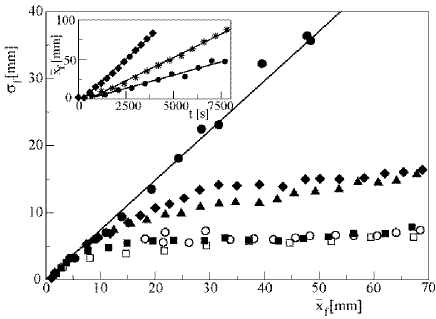
Figure 8: Variation of the fronts width $\sigma_{f}$ as function of the mean front position $\overline{x_{f}}$. Empty symbols stand for stable configurations, filled symbols for unstable ones. Squares, triangles, diamonds and circles correspond respectively to $|N_{g}|=0.00125$, $0.02$, $0.04$ and $0.2$. Inset: variation of $\overline{x_{f}}$ as a function of time in the unstable configuration for $N_{g}=-0.2$ ($\bullet$), $N_{g}=-0.08$ ($\ast$) and $N_{g}=-0.04$ ($\blacklozenge$). Solid lines: linear regressions on data points.

The variation of $\sigma_{f}$ with $\overline{x_{f}(t)}$ depends also strongly on the value of $N_{g}$ (Fig. 8). At the highest mean flow velocity (i.e. $|Ng|=0.00125$), $\sigma_{f}$ becomes constant and equal to $6\,\mathrm{mm}$ as soon as the distance from the injection line is larger than $10\,\mathrm{mm}$. This value is the same for both stable and unstable flow configurations: this is in agreement with the qualitative observations of Sec. III.1 in which no influence of buoyancy is visible when comparing Figs. 1c and 1f.

In contrast, at low flow rates (or large $|N_{g}|$ values), the large differences between the corresponding concentration maps in Fig. 1 are reflected in the variations of $\sigma_{f}$ with $\overline{x_{f}}$. At the lowest flow-rate ($|N_{g}|=0.2$), $\sigma_{f}$ keeps increasing roughly linearly with $\overline{x_{f}}$ in the unstable case; in the stable configuration, in contrast, $\sigma_{f}$ reaches quickly a limit of the same order of magnitude as for the highest velocity. At the intermediate velocities ($N_{g}=0.02-0.04$), the limiting value of $\sigma_{f}$ is higher in the unstable configuration than both in the stable one and at the highest velocity. The distance $\overline{x_{f}}$ required to reach this limit is also increased.

This result suggests that, in the unstable configuration and for intermediate $N_{g}$ values ($-0.01>N_{g}\geq-0.1$), two distinct regimes are successively observed. At short distances, the displacement is controlled by the instability while the variation of $\sigma_{f}$ is similar to that measured for $N_{g}=-0.2$. At larger distances, the variation of $\sigma_{f}$ levels off and it reaches a nearly constant value like for stable displacements. The transition distance increases with $N_{g}$: for $N_{g}=-0.2$, it is of the order of the sample length, explaining why the second regime is not observed. Together with results reported previously, we use biw this observation to provide an analytical estimation of the dispersivity for $N_{g}<-N_{g}^{c}$.

In order to compare the results of the present section III.4 with those of section III.3, it must be emphasized that $\sigma_{f}$ refers to the extension of the iso concentration front $c=0.5$ in the flow direction: it does not include therefore the influence of the width of the concentration profile at a given transverse distance $y$. At high velocities, for instance, the iso concentration front is nearly flat (Fig. 7a) and displays only a few spikes. In this case, $\sigma_{f}$ reaches a non-zero limit at long distances (due to these small features) and it does not increase as $t^{0.5}$ like the global width of the mean concentration profile discussed in Sec.III.3. In the unstable cases and at low velocities, the linear increase of $\sigma_{f}$ at long distances reflects directly the buoyant rise of fingers: its dynamics differs from that of the global spreading of the mixing zone. The latter results from the combination of several mechanisms (including, but not exclusively, the growth of the fingers) leading to an increase of the global width of the concenration profile as $t^{0.5}$.

IV Estimation of dispersivity variations for unstable displacements

The development of fingers driven by buoyancy forces in the unstable configuration is opposed by lateral mixing induced by transverse dispersion: it reduces the local density contrast $\delta\rho$ between the fingers and the surrounding fluid and, finally, the buoyancy forces. As pointed out in Sec.III.4, the structure of the displacement front has a characteristic size $\lambda$ constant and close to $4\ mm$ for gravity numbers in the range $-0.01>N_{g}>-0.2$. The characteristic exchange time $\tau$ for lateral mixing will then be of the order of the transverse diffusion time across the half-width $\lambda/2$ with:

$$\tau=\frac{\lambda^{2}}{8D_{\perp}}$$ (6)

in which $D_{\perp}$ is the transverse dispersion coefficient.

The rising motion of the fingers driven by buoyancy forces should have a velocity $u_{finger}$ proportional to the local density contrast with $u_{finger}\sim(\delta\rho/\Delta\rho U_{g})$. Assuming that $\delta\rho$ decreases exponentially with a time constant of the order of the transverse mixing time $\tau$ leads to $u_{finger}\sim U_{g}\,exp(-t/\tau)$. The vertical displacement $l(\tau)$ of the rising finger before its velocity goes to zero should then be given by:

$$l(\tau)\simeq\tau U_{g}.$$ (7)

$l(\tau)$ is then the typical spreading distance of the front due to buoyancy driven motions during the time $\tau$: it should be of the same order of magnitude as the limiting value of the width $\sigma_{f}$ of the iso concentration lines at long distances. The transverse dispersion coefficient $D_{\perp}$ generally decreases with the Péclet number (or equivalently with the flow velocity $U$) so that both $\tau$ and $l(\tau)$ should increase at low velocities. This agrees with the observed increase of $\sigma_{f}$ at long distances. At very low velocities, $l(\tau)$ will reache (or exceed) the system size: this is indeed observed at the lowest experimental flow velocity ($N_{g}=-0.2$). In that case, $\sigma_{f}$ keeps increasing with distance and does not reach a constant value within the model length.

In order to estimate the dispersion coefficient component $D_{buoyancy}$ associated to these buoyancy driven motions, one may consider $\tau$ represents as the characteristic crossover time towards diffusive front spreading: the corresponding width $l(\tau)$ should then verify $l(\tau)^{2}\simeq\,2D_{buoyancy}\tau$. Combining with Eqs. (6) and (7), this leads to the following value for the dispersivity component $l_{d\ buoyancy}$:

$$l_{d\ buoyancy}=\frac{D_{buoyancy}}{U}=\frac{U_{g}^{2}\lambda^{2}}{16UD_{\perp}}.$$ (8)

As a first approximation, the total dispersivity $l_{d}$ is considered to be the sum of the dispersivity $l_{d}^{eq}$ for a fully passive tracer and of $l_{d\ buoyancy}$: this amounts to assume that these two dispersion processes are independent. This assumption us only an approximation since the spatial flow velocity variations in the model influence both spreading processes.

The normalized passive tracer dispersivity $l_{d}^{eq}/a$ may be estimated from data obtained with the polymer solutions for which, as noted above, no buoyancy effect is visible. The equation:

$$\frac{l_{d}^{eq}}{a}\simeq fPe^{\alpha}$$ (9)

where $\alpha=0.35\,\pm\,0.03$ and $f=1.5\,\pm\,0.3$ has been selected for that purpose: it provides indeed a good global fit (dashed line in Figure 6) with the polymer data at all $Pe$ values and an acceptable one with water-glycerol data either in the stable configuration or at high velocities.

Combining Eqs. (8-9) and replacing $U$ by its expression as a function of $Pe$ leads then to:

$$\frac{l_{d}}{a}=fPe^{\alpha}+\frac{U_{g}^{2}\lambda^{2}}{16\epsilon Pe^{1+\beta_{T}}D_{m}^{2}}$$ (10)

in which $\epsilon$ is a constant. In this equation the transverse dispersion coefficient $D_{\perp}$ is assumed to vary as: $D_{\perp}=D_{m}\epsilon Pe^{\beta_{T}}$ as suggested by numerical simulations from ref. bruderer01 for networks of capillaries of random radii.

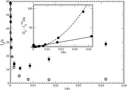
Figure 9: Variation of $l_{d}/a$ as function of $1/Pe$ for the water-glycerol solution. Filled (resp. empty) circles correspond to $N_{g}<0$ (resp. $N_{g}>0$). Inset : Variation of $(l_{d}-l_{d}^{eq})/a$ as function of $1/Pe$ for unstable experiments in a $2D$ network ($\bullet$) and a $3D$ porous medium ($\blacksquare$) freytes01 . In order to make comparisons easier, horizontal (resp. vertical) values for $3D$ data have been divided by a factor $5$ (resp. $0.6$). Solid (resp. dotted) lines: regressions using power laws of exponents $1$ (resp. $2.1$).

In order to put more emphasis on the buoyancy controlled regime at low flow velocities (low $Pe$), the variation of the dispersivity is plotted in Figure 9 as function of $1/Pe$. For unstable flows, as soon as $1/Pe>0.0025\,(1/400)$, $l_{d}$ steadily increases with $1/Pe$. This is also the case of the buoyancy component estimated by subtracting the passive tracer dispersivity component $l_{d}^{eq}$ from the values of $l_{d}$. The difference $l_{d}-l_{d}^{eq}$ increases linearly with $1/Pe$ and can be fitted by the second term of Eq. (10) with $\epsilon=0.3$ and $\beta_{T}\simeq 0$ (continuous line in the inset of Figure 9).

The experimental value of $\beta_{T}$ is lower than that reported in ref. bruderer01 ($\beta_{T}=0.2$); this result corresponds to numerical simulations for capillary tube networks with a normalized standard deviation $\sigma_{a}/a$ of the channel aperture equal to that of ours ($\sigma_{a}/a=0.3$). However, in our experiments, the influence of the $l_{d\ buoyancy}$ term is mostly significant at the lower Péclet numbers ($Pe\leq 50$) while the simulations of ref. bruderer01 deal with $Pe\geq 300$. The variation of $D_{\perp}$ for $Pe\leq 50$ may therefore be expected to be slower (and the corresponding exponent lower) due to the influence of the molecular diffusion coefficient $D_{m}$ which represents a constant lower limit at very low Péclet numbers.

In the present work, the variation of the coefficient of dispersion $D$ results directly from the 2D nature of the network which has been used. In a 3D porous medium, a bead packing for instance, $D$ depend weakly on the Péclet number dullien91 ; freytes01 ; flowers2007 . In this case $\beta_{T}$ and $\alpha$ are usually report to be equal and to range between $1$ and $1.2$ sahimi95 . As a result, the difference $l_{d}-l_{d}^{eq}$ estimated from the model is expected to increase with $Pe$ like $\simeq 1/Pe^{2}$. We have tested this prediction is tested by re-analyzing the dispersion coefficients measured by Freytes et al freytes01 . In this work, gravity driven instabilities were studied in a model porous packing of $1\ mm$ glass beads and for a density difference $\Delta\rho=10^{-3}g/l$. For water and in the high $Pe$ regime where the effect of buoyancy is negligible, their data show that : $l_{d}^{eq}\propto Pe^{0.1\pm 0.1}$ indicating that $\beta_{T}\simeq 1.1\pm 0.1$. As above, the buoyancy component is estimated by subtracting the passive tracer dispersivity $l_{d}^{eq}$ from the measured dispersivities. The difference $l_{d}-l_{d}^{eq}$ obtained in this way is found to vary as $(1/Pe)^{1.9\pm 0.2}$ (see inset of Fig. 9) with an exponent $1.9$ close to the value $1+\beta_{T}\simeq 2.1\,\pm\,0.1$. predicted by the model

V Conclusions

To conclude, the miscible vertical displacement measurements on transparent networks of channels reported here have provided information at both the local and macroscopic scales on the mixing front of two miscible fluids of slightly different densities. Qualitatively, the present macroscopic dispersion measurement confirm previous ones performed on three-dimensional porous media flowers2007 : the key feature of this work is that additional new information is provided by the high resolution visualization of front structures of different sizes down to the scale of individual channels. Using this information, the front distortions resulting from instabilities in unstable density contrast configurations could be analyzed quantitatively.

In these systems, the global spreading of the front results from the combination of the effects of the disordered spatial variations of the velocity field (only mechanism active in the passive tracer case) and of buoyancy driven flows; the latter may either decrease or reduce the dispersion depending on the gravitationally stable or unstable configuration of the fluids. For large Péclet numbers ($Pe>500$) (i. e. small gravity numbers $|N_{g}|<0.01$), the displacement fronts are very similar in both configurations and the global shape of the iso-concentration fronts is flat. In this case, the front spreading characteristics and the dispersivity values are similar to those measured for shear-thinning polymer solutions.

In the stable configuration, the dispersivity decreases significantly for $Pe<500$ and becomes constant and close to $1\ mm$ when $Pe<100$. At the same time, the geometry of the iso-concentration front is only weakly affected by the stabilizing effect of buoyancy.

In the unstable configuration, and at moderate $N_{g}$ values (e.g. $-0.01>N_{g}>-0.2$), the initial development of the instabilities is damped by transverse hydrodynamic dispersion after some time. As a result, front spreading remains dispersive but with a dispersivity increasing at low velocities as $l_{d}\simeq 1/Pe$. These instability fingers are reflected in the geometry of the iso-concentration fronts which display large spikes and troughs. In this range of $N_{g}$ values, the location (in the transverse direction) and the width of the spikes are observed to be constant. The spreading in the flow direction as a function of time displays two regimes: initially (short distances from the injection), the width of the iso-concentration fronts increases linearly and, then, it levels-off towards a constant value at large distances.

In order to explain these results, an approach combining the influences of longitudinal buoyancy forces parallel to the mean flow and of the exchange of solute between the instability fingers and the surrounding fluid has been developed. It allows one to account semi-quantitatively for the dependence of the dispersivity on the Péclet number if $N_{g}>-0.2$. The present experimental observations on $2D$ networks as well as previous measurements on $3D$ bead packings (for which $l_{d}\simeq 1/Pe^{2}$) are well fitted by the model.

At the lowest flow velocity investigated ($N_{g}=-0.2$), large fingers develop on the interface; the concentration front is strongly distorted but its spreading can still be considered as dispersive. Yet, the number of fingers on the iso-concentration front decreases with time while its width parallel to the flow keeps increasing with distance. This suggests that, above this gravity number, gravitational instabilities might control the transport process. In 3D porous media, a linear growth of the mixing zone reflecting the dominant influence of such instabilities is only observed above a higher threshold value $N_{g}\simeq-1.5$ menand05 .

Further studies will be needed to confirm our observation by using pairs of fluids with different density contrasts. Another issue of practical interest is the influence of the viscosity contrast on the spatial distribution of the tracer.

References

- (1) J. Bear, “Dynamics of Fluids in Porous Media”, Elsevier Publishing Co., New York (1972).
- (2) F.A.L. Dullien, “Porous Media, Fluid Transport and Pore Structure”, 2nd edition, Academic Press, New York (1991).
- (3) M. Sahimi, “Flow and Transport in Porous Media and Fractured Rock”, VCH, Weinheim, Chapt. 12 (1995).
- (4) E. Charlaix, J.P. Hulin, C. Leroy and C. Zarcone. “Experimental study of tracer dispersion in flow through two-dimensional networks of etched capillaries,” J. Phys. D: Appl. Phys. 21, 1727 (1988).
- (5) M.A. Freytes, A. d’Onofrio, M. Rosen, C. Allain, J.P. Hulin. “Gravity driven instabilities in miscible non Newtonian fluid displacements in porous media.” Physica A 290, 286 (2001).
- (6) C. Oltean, Ch. Felder, M. Panfilov and M.A. Bués, “Transport with a very low density contrast in Hele Shaw cell and porous medium: evolution of the mixing zone,” Transport Porous Media 55, 339–360 (2004).
- (7) T. Menand and A.W. Woods, “Dispersion, scale, and time dependence of mixing zones under gravitationally stable and unstable displacements in porous media,” Water Resour. Res. 41, W05014 (2005).
- (8) T.C. Flowers and J.R. Hunt, “Viscous and gravitational contributions to mixing during vertical brine transport in water-saturated porous media,” Water Resour. Res. 43, W01407 (2007).
- (9) R.A. Schincariol, F.W. Schwartz and C.A. Mendoza, “Instabilities in variable density flows: stability and sensitivity analyses for homogeneous and heterogeneous media,” Water Resour. Res. 33, 31–41 (1997).
- (10) M. Beinhorn, P. Dietrich and O. Kolditz, “3-D numerical evaluation of density effects on tracer tests,” J. Contam. Hydrol. 81, 89–105 (2005).
- (11) K. Johannsen, S. Oswald, R. Held and W. Kinzelbach, “Numerical simulation of saltwater-freshwater fingering instabilitites observed in a porous medium,” Adv. Water Resour. 29, 1690–1704 (2006).
- (12) R. Lenormand, C. Zarcone and A. Sarr, “Mechanism of the displacement of one fluid by another in a network of capillary ducts,” J. Fluid Mech. 135, 337 (1983).
- (13) V. D’Angelo, H. Auradou, C. Allain, J-P Hulin, “Pore scale mixing and macroscopic solute dispersion regimes in polymer flows inside 2D model networks,” Phys. Fluids 19, 033103 (2007).
- (14) P.Z. Wong, Ed. “Methods in the physics of porous media,” Experimental methods in the physical sciences 35, Academic Press, London (1999).
- (15) V. Kretz, P. Berest, J.P. Hulin, D.Salin, “An experimental study of the effects of density and viscosity contrasts on macrodispersion in porous media,” Water Resour. Res. 39, 1032-1041 (2003).
- (16) S. Tenchine and Ph. Gouze, “Density contrast effects on tracer dispersion in variable aperture fractures,” Adv. Water Resour. 28, 273–289 (2005).
- (17) A. Boschan, H. Auradou, I. Ippolito, R. Chertcoff and J.P. Hulin, “Miscible displacement fronts of shear thinning fluids inside rough fractures,” Water Resour. Res. 43, W03438 (2007).
- (18) H.H. Liu and J.H. Dane, “A Criterion for gravitational instabilities in miscible dense plumes,” J. Contam. Hydrol. 23, 233–243 (1996).
- (19) C. Welty and L. W. Gelhar, “Stochastic analysis of the effects of fluid density and viscosity variability on macrodispersion in heterogeneous porous media,” Water Resour. Res. 27, 2061– 2075 (1991).
- (20) R.A. Wooding, “Growth of fingers at an unstable diffusing interface in a porous medium or Hele-Shaw cell,” J. Fluid Mech. 39, 477–495 (1969).
- (21) C. Bruderer and Y. Bernabé, “Network modeling of dispersion: transition from Taylor dispersion in homogeneous networks to mechanical dispersion in very heterogeneous ones,” Water Resour. Res. 37 (4), 897–908 (2001).