From the hyperbolic $24$-cell to the cuboctahedron

Abstract.

We describe a family of $4$-dimensional hyperbolic orbifolds, constructed by deforming an infinite volume orbifold obtained from the ideal, hyperbolic $24$-cell by removing two walls. This family provides an infinite number of infinitesimally rigid, infinite covolume, geometrically finite discrete subgroups of $\text{Isom}(\mathbb{H}^{4})$. It also leads to finite covolume Coxeter groups which are the homomorphic image of the group of reflections in the hyperbolic $24$-cell. The examples are constructed very explicitly, both from an algebraic and a geometric point of view. The method used can be viewed as a $4$-dimensional, but infinite volume, analog of $3$-dimensional hyperbolic Dehn filling.

1. Introduction

The study of hyperbolic manifolds or, more generally, discrete subgroups of isometries of hyperbolic space, typically divides along dimensional lines, between dimension $2$ where there are deformations of co-compact respresentations and higher dimensions where there are no such deformations due to Mostow rigidity. However, there is an equally important distinction between dimension $3$ and higher dimensions. While Mostow-Prasad rigidity [Mos, Pr] (or Calabi-Weil local rigidity [C, We]) guarantees that there are no nontrivial families of complete, finite volume structures in dimension at least $3$, if either the completeness or finite volume hypothesis is dropped, in dimension $3$ there typically are deformations.

Specifically, a noncompact, complete, finite volume hyperbolic $3$-manifold $M$ with $k$ cusps always has a $k$–complex dimensional deformation space, through necessarily non-complete hyperbolic structures. Topologically, $M$ is the interior of a compact $3$-manifold $\bar{M}$ with $k$ torus boundary components. Certain of the nearby incomplete structures, when completed, give rise to complete hyperbolic structures on closed $3$-manifolds which are obtained topologically by attaching solid tori to the torus boundary components of $\bar{M}$. This process is called hyperbolic Dehn filling. There are an infinite number of topologically distinct ways to attach a solid torus to each boundary component and a fundamental result of Thurston’s [Th, Ch.5] is that, if a finite number of fillings are excluded from each boundary component, the remaining closed manifolds have hyperbolic structures. In particular, the process of hyperbolic Dehn filling gives rise to an infinite sequence of closed hyperbolic $3$-manifolds whose volumes converge to that of the cusped hyperbolic structure $M$.

This is in marked contrast with the situation in dimension at least $4$ where a central result of Garland and Raghunathan [GR] implies that a finite covolume discrete subgroup of $\text{Isom}(\mathbb{H}^{n}),~{}n\geq 4$, is isolated, up to conjugacy, in its representation variety. (Their result applies, in fact, to a much more general class of Lie groups.) In particular, there are no nontrivial deformations of a finite volume hyperbolic structure, even through incomplete structures, in dimension $4$ and higher; there is no higher dimensional analog of hyperbolic Dehn filling for finite volume structures. This is reflected by a result of Wang [Wa] which states that, for any $V$ and fixed $n\geq 4$, there are only a finite number of hyperbolic $n$-manifolds with volume at most $V$.

There is an equally dramatic distinction between dimension $3$ and higher dimensions for infinite volume, geometrically finite hyperbolic structures. When there are no parabolic elements, these structures can be compactified by adding boundary components that inherit conformally flat structures from the sphere at infinity. In dimension $3$ these will consist of surfaces of genus at least $2$ and Ahlfors-Bers deformation theory [And] guarantees that the deformation space of such structures has dimension equal to the sum of the dimensions of the Teichmuller spaces of conformal structures on the boundary surfaces. By contrast, in higher dimensions the $(n-1)$-dimensional boundary can have a large dimensional space of conformally flat deformations while the $n$-dimensional hyperbolic structure is locally rigid; i.e., none of the deformations of the boundary representation in $\text{Isom}(\mathbb{H}^{n})$ extend over the interior. In this paper we will construct an infinite family of examples with this property.

In dimension $3$ the situation can be summed up in both the finite volume and the infinite volume, geometrically finite cases by saying that a half-dimensional subset of deformations of the boundary representations (up to conjugacy) extends over the entire $3$-manifold. In higher dimensions, there are no deformations of finite volume complete structures, even through incomplete structures, and there is no general theory of deformations in the infinite volume case. As a result, the study of hyperbolic structures in dimension $4$ and higher currently consists largely of constructing and analyzing examples. This paper can be viewed as fitting into that context. However, we believe that the method we use to construct these examples should be applicable in much more general situations.

We will describe an infinite collection of $4$-dimensional hyperbolic orbifolds. They are actually part of a continuous family of representations into $\text{Isom}(\mathbb{H}^{4})$, each of which corresponds to a singular hyperbolic structure, called a cone manifold. Within this continuous family there are an infinite number of geometrically finite discrete subgroups which are infinite covolume but infinitesimally rigid. The process we use to create this family can be viewed as a $4$-dimensional, but infinite volume, analog of hyperbolic Dehn filling. As such it can be viewed as an attempt to mimic, to as great an extent possible, the situation in dimension $3$ and to provide some insight into what a general theory of deformations in dimension $4$ might look like.

The examples are all reflection groups; the discrete groups are hyperbolic Coxeter groups. The point of departure is the ubiquitous $24$-cell in its realization as a right-angled, ideal $4$-dimensional hyperbolic polytope. We denote the group of reflections in the $3$-dimensional walls of this polytope by $\Gamma_{24}$. It is a finite volume discrete subgroup of $\text{Isom}(\mathbb{H}^{4})$. By the Garland-Raghunathan theorem it has no deformations. However, when we remove the reflections in two disjoint walls (we will be more explicit later about which walls), the resulting reflection group $\Gamma_{22}$ with infinite volume fundamental domain becomes flexible. We prove that there is a smooth $1$-dimensional family of representations of $\Gamma_{22}$ which corresponds to a family of polytopes in $\mathbb{H}^{4}$. These are all the possible deformations of $\Gamma_{22}$ near the inclusion representation. Geometrically, certain pairs of walls that had been tangent in the original polyhedron pull apart a finite nonzero distance, and other previously tangent pairs of walls intersect. The polytopes retain a large degree of symmetry. All the new angles of intersection are equal and the walls which previously intersected orthogonally continue to do so. The new angle of intersection, denoted by $\theta$, can be used as a parameter for the family of representations, which we denote by $\rho_{\theta}$.

When $\theta=\pi/m$, the group of reflections in the walls of the polytope is a discrete subgroup of $\text{Isom}(\mathbb{H}^{4})$. It is a homomorphic image of $\Gamma_{22}$ with new relations that do not exist in $\Gamma_{22}$. In fact, because of the symmetry retained throughout the family, it is possible to conclude that, even when $\theta=\frac{2\pi}{n}$, where $n\geq 3$ is an integer, the group $\rho_{\theta}(\Gamma_{22})$ is discrete.

Both $\Gamma_{24}$ and $\Gamma_{22}$ are right-angled Coxeter groups. Although $\Gamma_{22}$ is most naturally viewed as a subgroup of $\Gamma_{24}$, a well-known property of right-angled Coxeter groups implies that it is also a quotient group of $\Gamma_{24}$. Since the above discrete groups are all quotients of $\Gamma_{22}$ we obtain surjections of $\Gamma_{24}$ onto them for any $n\geq 3$.

We can summarize the main results of this paper as:

Theorem 1.1.

Let $G$ be the isometry group of hyperbolic $4$-space. There is a discrete geometrically finite reflection group $\Gamma_{22}<G$ and a smooth family of representations $\rho_{\theta}:\Gamma_{22}\rightarrow G$ converging algebraically, as $\theta\to 0$, to the inclusion map. The family has the following properties:

1. When $\theta=\frac{2\pi}{n}$, where $n\geq 3$ is an integer, the representation $\rho_{\theta}$ is not faithful. The image group $\Lambda_{n}:=\rho_{\theta}(\Gamma_{22}),\theta=\frac{2\pi}{n}$ is a discrete geometrically finite subgroup of $G$.

2. In the representation variety $\text{Hom}(\Lambda_{n},G)$ the inclusion map is infinitesimally rigid for all $n\geq 3$.

3. When $n=2m$, $m\geq 4$, $\Lambda_{n}$ has infinite covolume. Its convex core does not have totally geodesic boundary.

4. When $n=2m$, $m\geq 4$, the boundary subgroups of $\Lambda_{m}$ are convex cocompact and have nontrivial discrete faithful convex cocompact deformations.

5. For all $n\geq 3$, there is a surjective homomorphism from the reflection group in the regular, ideal hyperbolic $24$-cell, $\Gamma_{24}$, onto $\Lambda_{n}$.

Representations in this family exist for $\theta\in[0,\pi]$, and they correspond to convex $4$-dimensional polytopes for $\theta\in[0,\pi)$. For all $\theta\in(0,\pi/3)$ they are combinatorially the same; only certain angles vary. However, beginning at $\frac{\pi}{3}$, there is a fairly drastic change in the combinatorics and for $\theta\in[\cos^{-1}(1/3),\pi)$, the polytope has finite volume.

The finite covolume discrete groups $\Lambda_{n}$ in this family, when $n=3,4,5$, are of particular interest; so is the case when $n=6$. At $\theta=\pi/3$, when $n=6$, the topology of the boundary of the convex hull changes and the resulting boundary components become totally geodesic. This is reminscent of the familiar process in dimension $3$ when curves on a higher genus boundary surface are pinched, resulting in boundary components that are all totally geodesic triply punctured spheres. However, unlike the triply punctured sphere case, the boundary components in our situation have non–totally geodesic representations. At $\theta=\cos^{-1}(1/3)\approx 1.231$ the boundary components of the polytopes completely disappear and for all larger values of $\theta$ the polytopes have finite volume. In particular, when $n=3,4,5$ the groups $\Lambda_{n}$ are actually finite covolume discrete reflection groups. Using a criterion of Vinberg [Vin2] we can decide whether or not they are arithmetic.

Finally, as $\theta\to\pi$ the $4$-dimensional polytopes collapse to a $3$-dimensional hyperbolic ideal polyhedron, the right-angled cuboctahedron. This is the end of the path referred to in the title of this paper.

Theorem 1.2.

Let $\rho_{\theta}:\Gamma_{22}\rightarrow G$ be the family of representations in Theorem 1.1 and let $\Lambda_{n}:=\rho_{\theta}(\Gamma_{22}),\theta=\frac{2\pi}{n}$ be the image groups where $n\geq 2$ is an integer.

1. When $n=3,4,5$ the discrete groups $\Lambda_{n}$ have finite covolume. They are non-uniform lattices.

2. When $n=3,4$ the lattice $\Lambda_{n}$ is arithmetic. When $n=5$ it is not arithmetic.

3. When $\theta=\pi$ the image group $\rho_{\pi}(\Gamma_{22})$ preserves a $3$-dimensional hyperplane, and has a degree two subgroup conjugate into $\text{Isom}(\mathbb{H}^{3})$ as the group of reflections $\Gamma_{co}$ in the ideal right-angled cuboctahedron.

The results in Theorems 1.1 and 1.2 are proved throughout the body of the paper; the theorems themselves will not reappear explicitly outside of this introductory section. Hence, we will provide here an outline of the paper with a guide to where the various results are proved.

Section 2 provides some background material on reflection groups, Zariski tangent spaces and orbifolds. In Section 3 we give a detailed introduction to the geometry and combinatorics of the hyperbolic $24$-cell, emphasizing the aspects used throughout the paper. In Section LABEL:symmetries we describe the symmetries of the $24$-cell, focusing on those that remain even after we remove two walls to create the flexible reflection group $\Gamma_{22}$. We will ultimately find that all deformations of $\Gamma_{22}$ preserve this group of symmetries, a fact that simplifies a number of the proofs. In Section LABEL:deformation_prelims we discuss the deformation theory of some auxillary subgroups of $\Gamma_{22}$.

In Section LABEL:defining_the_deformation_2 we explicitly construct the family of representations $\rho_{\theta}$ of the reflection group $\Gamma_{22}$. Throughout the paper we use a different parameter $t$ because it is easier to write down the deformation using this parameter instead of the angle $\theta$. The formula relating the two parameters appears in Proposition LABEL:angle_prop. This, together with an easy application of the Poincare fundamental domain lemma, gives a proof of the existence of the infinite family of discrete reflection groups as stated in part 1 of Theorem 1.1. The family of representations is constructed by first assuming that the symmetries of the polytope $P_{22}$ obtained by removing two walls of the $24$-cell are preserved by the deformation. We show that the representations in our family are the only ones preserving this group of symmetries. It is only much later, in Sections LABEL:inf_letter and LABEL:computing_infinitesimally, where we show that in fact all deformations preserve these symmetries and, hence that we have constructed all possible local deformations. This is used to prove the smoothness of the family as well as the infinitesimal rigidity of the groups $\Lambda_{n}$ (which is part (2) of Theorem 1.1). Because the proof of these results is a fairly complicated computation of Zariski tangent spaces, we have postponed it until after we have analyzed the geometry of the family.

In Sections LABEL:viewed_in_the_sphere_at_infinity and LABEL:fundamental_domain we analyze the geometry of the polytopes corresponding to the representations in our family. The geometric and combinatorial aspects of the polytopes and their walls are not at all apparent from the explicit description of the family which is given simply as a family of space-like vectors corresponding to the hyperplanes that determine the walls of reflection. This analysis is necessary in order to make further conclusions about the discrete reflection groups in the family. Since it focuses on the geometry of the various walls, which are $3$-dimensional, it also provides a link between the $3$ and $4$ dimensional deformation theories. The results of these sections hold for angles $\theta$ strictly between $0$ and $\pi/3$; in this range the combinatorics of the walls is constant. Using this analysis, in Section LABEL:miscellaneous_section we prove parts (3) and (4) of Theorem 1.1.

In Section LABEL:disappear we begin the description of the more intricate change in the combinatorics and geometry of the polytopes that occurs between angles $\pi/3$ and $\pi/2$. During this period the combinatorics of the infinite volume ends of the polytopes change and then these ends completely disappear. We provide a series of floating point based diagrams that suggest how this process occurs. In Section LABEL:manual_lattice we give a rigorous proof of this process. The proof depends on passing to representations of the extended group $\widetilde{\Gamma}_{22}$ where the finite group of reflective symmetries have been added in. This group has fewer generators (though more complicated walls), allowing for a manageable analysis of the Coxeter diagrams of the image groups $\rho_{\theta}(\widetilde{\Gamma}_{22})$. In this latter section, part (5) of Theorem 1.1 and parts (1) and (2) of Theorem 1.2 are proved. In Section LABEL:cubeoctahedron_section we analyze the process of converging to the terminal group $\rho_{\pi}(\Gamma_{22})$ and its relation to the cuboctahedron reflection group.

Finally, it is perhaps worth mentioning that this paper is not a completely accurate reflection of the process by which we discovered the family of polytopes described here. Our presentation represents an assimilation of the material after attempting to understand initial computations in direct geometric terms, both contrasting it with and drawing analogies to the general $3$-dimensional theory. Originally, we found the family of examples by a combination of computational and graphical experimentation, both computer-aided. After removing one and then two walls from the $24$-cell, we computed the dimension of the Zariski tangent space to the deformation space to be $1$-dimensional in the latter case. We then attempted to construct an actual deformation corresponding to this Zariski tangent space. Rigorous computer-aided integer polynomial computation provided the proof of the existence of a substantial subinterval of our current family. However, after better understanding the geometry of this family and its symmetries, the use of the computer was removed from the proof. The only remnants of the computer assistance are the floating point diagrams in Section LABEL:disappear (which are rigorously confirmed in a later section) and the numerous pictures which we continue to find useful.

The authors benefited tremendously from the help of Daniel Allcock. In particular, his insights into the symmetries of the right-angled Coxeter group $\Lambda_{4}$ and how they can be made apparent by a particular choice of the space-like vectors in Minkowski space led directly to a significant simplification of our proofs. We would also like to thank Igor Rivin for several helpful conversations on topics related to the original computer-aided computations. Also thanks to Ian Agol and Alan Reid for their help in understanding Vinberg’s work on arithmetic reflection groups.

2. Preliminaries

In this section we will introduce some of the basic concepts and terminology that will be used throughout the paper.

2.1. Hyperbolic reflection groups

In this paper we will be studying $4$-dimensional hyperbolic reflection groups. A reflection group is, by definition, generated by elements $\{r_{i}\}$ of order $2$ with relations of the form $\{(r_{i}r_{j})^{m_{ij}}\}$, where $i\neq j$ and $m_{ij}\geq 2$ are integers. In some texts, the convention $m_{ij}=\infty$ is used to signify that the element $r_{i}r_{j}$ is of infinite order; however, in this case we will simply omit any relation between $r_{i}$ and $r_{j}$.

An $n$-dimensional hyperbolic representation of a reflection group $\Gamma$ is a representation of $\Gamma$ in the group $G_{n}$ of isometries of hyperbolic $n$-space. We will further require that the generators $r_{i}$ of $\Gamma$ are represented by reflections in codimension-$1$ totally geodesic hyperplanes. We do not generally require the group generated by these reflections to be discrete.

It is worth emphasizing that our requirement that the generators of $\Gamma$ are sent to reflections in hyperplanes is an extra assumption. Since there are other types of order two elements in $G_{n}$, such representations may not include all representations of $\Gamma$ into $G_{n}$. However, since any order two element in $G_{n}$ near a reflection in a hyperplane is again such a reflection, this restriction is not important locally. Any representation near one of this form still has the same property. In fact, because the set of reflections in hyperplanes is a connected component of the closed subset of elements of order two in $G_{n}$, the set of such hyperbolic representations is actually a union of components of the entire representation variety of $\Gamma$. Throughout this paper, a hyperbolic representation will mean a representation of $\Gamma$ in $G_{n}$ of this particular type.

We will be using the Minkowski model of hyperbolic space and restrict our attention to the case $n=4$ since that is the dimension most relevant to this paper. The Minkowski metric on $\mathbb{R}^{5}$ is determined by the inner product

$$(v,w):=-v_{0}w_{0}+v_{1}w_{1}+v_{2}w_{2}+v_{3}w_{3}+v_{4}w_{4}.$$

The resulting Minkowski space is denoted by $\mathbb{R}^{1,4}$. Recall that a space-like vector has positive Minkowski squared norm, a light-like vector has Minkowski squared norm zero, and a time-like vector has negative Minkowski squared norm. Hyperbolic $4$-space $\mathbb{H}^{4}$ is defined as the set of points with Minkowski squared norm $-1$ and a positive $0^{\text{th}}$ coordinate.

We will denote the full isometry group of $\mathbb{H}^{4}$ simply by $G$. It is isomorphic to the two components of $O(1,4)$ which preserve the top component of the hyperboloid of points with Minkowski squared norm $-1$. Viewing $O(1,4)$ as a subset of $5\times 5$ matrices, it is an affine algebraic variety in $\mathbb{R}^{25}$. Similarly, a finite presentation of a group $\Gamma$ gives the representation variety $\text{Hom}(\Gamma,G)$ the structure of a real algebraic variety. Specifically, if $\Gamma$ is generated by $k$ elements with $\ell$ relations, the representation variety $\text{Hom}(\Gamma,G)$ is defined as the subset of $G^{k}\subset\mathbb{R}^{25k}$ satisfying the $25\ell$ polynomial equations produced by the relations.

Because of the large dimensions of the spaces involved, such varieties are quite complicated to study. However, in the case of a hyperbolic representation of a reflection group, there is a simple observation that significantly reduces the dimension of the space in which representation variety lives. (It still is generally quite large, however.) The observation is that a reflection in a hyperplane is uniquely determined by that hyperplane, and that a hyperplane is uniquely determined by a space-like vector in $\mathbb{R}^{1,4}$. More specifically, a hyperplane in $\mathbb{H}^{4}$ is a totally geodesic embedded copy of $\mathbb{H}^{3}$. The order two isometry of $\mathbb{H}^{4}$ defined by reflecting in a hyperplane is uniquely determined by that hyperplane and conversely, uniquely determines that hyperplane. In the Minkowski model, a hyperplane is given by the intersection with $\mathbb{H}^{4}$ of a linear $4$-dimensional subspace of $\mathbb{R}^{1,4}$. This linear subspace $W\subset\mathbb{R}^{1,4}$ is in turn determined by a space-like vector $q\in\mathbb{R}^{1,4}$ satisfying $(q,W)=0$. A reflection isometry of $\mathbb{H}^{4}$ is thus determined by such a vector $q$ and the choice of $q$ is unique up to multiplication by a nonzero scalar. A choice of vector $q$ can actually be interpreted as a choice of one of the two half-spaces bounded by the hyperplane or as a choice of orientation on the hyperplane. Multiplication by a positive scalar leaves this choice unchanged but it is flipped by multiplication by $-1$.

The relations $\{(r_{i}r_{j})^{m_{ij}}\}$ in a hyperbolic representation of reflection group can also be described by relations between such vectors. To see this, denote by $W_{i},W_{j}$ the reflection hyperplanes for the representatives of a pair of generators $r_{i},r_{j}$. When the hyperplanes are a positive distance apart, the element $r_{i}r_{j}$ represents translation by twice the distance between the hyperplanes along their common perpendicular geodesic. When the hyperplanes are tangent at infinity, the product is a parabolic translation. In either case, when $W_{i}$ and $W_{j}$ are disjoint, the product has infinite order. When they intersect (and are distinct), they do so in a codimension-$2$ geodesic subspace. The product $r_{i}r_{j}$ rotates around this subspace by twice the dihedral angle between the hyperplanes. Thus, a relation of the form $(r_{i}r_{j})^{m_{ij}}=e$ is equivalent to the condition that the corresponding hyperplanes intersect in angle equal to an integral multiple of $\frac{\pi}{m_{ij}}$. Locally, the particular integral multiple will be constant for each $\{i,j\}$ pair; in all of our examples, the angles will be exactly equal to $\frac{\pi}{m_{ij}}$.

A pair of hyperplanes $W_{i}$ and $W_{j}$ are determined by a pair of space-like vectors $q_{i}$ and $q_{j}$ as described above. The geometry of the hyperplane pair can be read from the geometry of the vectors $q_{i}$ and $q_{j}$. In particular, if $W_{i}$ and $W_{j}$ intersect, then the dihedral angle $\theta$ formed by the $q_{i}$ side of $W_{i}$ and the $q_{j}$ side of $W_{j}$ satisfies the equation

(2.1) $$\cos\theta=\frac{-(q_{i},q_{j})}{\sqrt{(q_{i},q_{i})(q_{j},q_{j})}}.$$

Similarly, if $W_{i}$ and $W_{j}$ do not intersect then the length $\ell$ of the shortest hyperbolic geodesic from $W_{i}$ to $W_{j}$ satisfies

(2.2) $$\cosh\ell=\frac{-(q_{i},q_{j})}{\sqrt{(q_{i},q_{i})(q_{j},q_{j})}}.$$

Note that the right hand sides of these equations are invariant under multiplication of the individual vectors by positive scalars. Multiplication of a vector by $-1$ corresponds to a change of side of its hyperplane; this is an orientation issue that is best suppressed for the moment.

This shows that a relation of the form $(r_{i}r_{j})^{m_{ij}}=e$ for a hyperbolic representation of a reflection group is equivalent to a quadratic polynomial relation between the entries of the corresponding space-like vectors, $q_{i},q_{j}$, if the latter are normalized to have unit (or fixed) Minkowski length. This unit normalization is also a quadratic condition.

Thus, it is possible to view the set of $4$-dimensional hyperbolic realizations of a reflection group with $k$ generators and $\ell$ relations (ignoring the $k$ relations stating the generators have order $2$) as a real algebraic variety in $\mathbb{R}^{5k}$ determined by $k+\ell$ polynomial equations.

2.2. Zariski tangent space and infinitesimal rigidity

It is generally quite complicated to describe the simultaneous solutions to a large number of polynomial equations in a large number of unknowns. As a result, one is quickly led to consider instead the corresponding infinitesimal problem. If one knows a point $x$ in the simultaneous solution space of a collection $P$ of polynomials, one can look for tangent directions at $x$ in which the system continues to be satisfied to first order. This is done by differentiating the polynomials at $x$ and solving the resulting linear system of equations. The linear solution space is called the Zariski tangent space of the set of polynomials at $x$. The more modern terminology is to consider $P$ as determining a scheme $SP$; this linear space is then called the Zariski tangent space to $SP$ at $x$. We will use the following simple formal definition:

Let $P=\{p_{\alpha}\}$ be a collection of real polynomials in $n$-variables. Let $x\in\mathbb{R}^{n}$ be a point where all of the $\{p_{\alpha}\}$ simultaneously vanish. Then the Zariski tangent space at $x$ of the scheme $SP$ is the linear space

$$T^{Z}_{x}SP:=\{v\in T_{x}\mathbb{R}^{n}\,|\ \textstyle\frac{d}{dt}\big{|}_{t=0}\,p_{\alpha}(x+tv)=0\ \text{for all}\ \alpha\}\subseteq T_{x}\mathbb{R}^{n}.$$

In our case we are primarily interested in the actual real algebraic variety $V$ in $\mathbb{R}^{n}$ where a collection of polynomials $P$ simultaneously vanish. While every polynomial in the ideal generated by the $P$ will certainly vanish on $V$, not every polynomial vanishing on $V$ is necessarily in this ideal. Consider the simple example of the single polynomial $p(x,y)=x^{2}$ in $\mathbb{R}^{2}$. The variety $V$ in this case is the $y$-axis where $x=0$. The polynomial $q(x,y)=x$ vanishes on $V$ but is not in the ideal generated by $x^{2}$. This can have an effect on the computation of the Zariski tangent space. For the scheme determined by $x^{2}$ it is $2$-dimensional at any point where $x=0$. The Zariski tangent space for $V$, where one uses a generating set for the ideal of polynomials vanishing on $V$ (in this example, $q(x,y)=x$) in the above definition, the dimension is $1$ at every point on $V$.

In this example, the variety $V$ is a smooth manifold and the Zariski tangent space to $V$ is isomorphic to that of the smooth manifold. This is generally not the case. A standard example is the variety $V$ (and scheme) in the plane determined by $p(x,y)=x^{2}-y^{3}$. At the origin, the Zariski tangent space to $V$ (and to the scheme) is $2$-dimensional. The variety is not smooth there. Most importantly, there are tangent directions in the Zariski tangent space that do not correspond to actual curves in $V$. An infinitesimal solution to the equations need not correspond to a path of actual solutions.

Fortunately, there is a criterion that deals with both of these issues, the difference between the scheme and variety Zariski tangent spaces, as well as the existence of a curve of solutions in any tangent direction. This criterion uses the implicit function theorem. If one can find a smooth manifold of the same dimension as the Zariski tangent space of the scheme through a point on the variety, it follows that the variety is a smooth manifold of that dimension in a neighborhood of the point. The two Zariski tangent spaces coincide with the tangent space of the manifold and every tangent vector corresponds to a smooth path of solutions.

We will provide details in Section LABEL:computing_infinitesimally, where this argument is used to analyze our nontrivial family of representations. However, it is worth pointing out a classical use of this argument, due to Weil, with respect to the concept of infinitesimal rigidity of a representation of a finitely presented discrete group $\Gamma$ into a Lie group $G$. Here $\Gamma$ and $G$ are quite general; it suffices, for example, for $G$ to be real algebraic. In particular, the argument applies to the situation considered in this paper.

With $\Gamma$ and $G$ as above, let $\rho$ be a representation in $\text{Hom}(\Gamma,G)$ which is a real algebraic variety (scheme). As in the previous section, it can be viewed as a subset of $G^{n}$ where $n$ is the number of generators of $\Gamma$. For $g\in G$ we can conjugate $\rho$ by $g$ to obtain the new representation $(g.\rho)(\gamma):=g\rho(\gamma)g^{-1}.$ We say that $\rho$ is infinitesimally rigid if the following is true: for any $v$ in the Zariski tangent space of $\text{Hom}(\Gamma,G)$ at $\rho$ there is a path $g(t)$ in $G$ such that $g(0)$ is the identity element and

$$\textstyle\frac{d}{dt}\big{|}_{t=0}\,(g(t).\rho)=v.$$

This condition is commonly described in terms of the vanishing of the cohomology group $H^{1}(\Gamma;\mathcal{G}_{\rho})$ where the coefficients are in the Lie algebra $\mathcal{G}$ of $G$, twisted by the representation $\rho$. The cocycles correspond to the Zariski tangent space and the coboundaries to those tangent vectors induced infinitesimally by conjugation.

The point of this definition is that infinitesimal rigidity means every infinitesimal deformation of $\rho$ is obtained as the tangent vector to a path of representations obtained via conjugation. Conjugate representations are not usually considered to be genuinely different representations of $\Gamma$. The representation $\rho$ is therefore considered to be rigid at the infinitesimal level.

Weil’s Lemma [We] implies that if the centralizer of $\rho$ in $G$ is trivial, so that conjugation by $G$ locally determines a manifold in $\text{Hom}(\Gamma,G)$ through $\rho$ with dimension equal to the dimension of $G$, then infinitesimal rigidity implies that near $\rho$ this manifold coincides with $\text{Hom}(\Gamma,G)$. Near $\rho$, $\text{Hom}(\Gamma,G)$ is a smooth manifold and all nearby representations are conjugate. The latter condition is called locally rigidity. Thus, under a mild assumption on the conjugation action at $\rho$, Weil’s Lemma implies that an infinitesimally rigid representation is locally rigid. The converse is occasionally false.

2.3. Orbifolds

The main topic of this paper is the representation space of a reflection group $\Gamma_{22}$ which has a discrete faithful $4$-dimensional hyperbolic representation coming from the group of reflections in the codimension-$1$ walls of an infinite volume polyhedron in $\mathbb{H}^{4}$. We will find a smooth $11$-parameter family of $4$-dimensional hyperbolic representations (not necessarily discrete) of this group. Dividing out by the conjugation action provides a smooth $1$-dimensional family of nontrivial deformations. As discussed in Section 2.1, this family will be described algebraically as a family of space-like vectors. However, it will also be described geometrically as a family of groups generated by reflections in a family of varying polyhedra. These polyhedra will have new intersections between walls not existing in the original polyhedron and the combinatorics of the polyhedra will change a couple of times during the family. At a countably infinite number of times all of the walls that intersect will do so at angles of the form $\pi/k$ for various integers $k$. In these cases, the group generated by reflections in the walls of the polyhedron will be discrete with the polyhedron as a fundamental domain. (This follows from Poincaré’s lemma, which is discussed in Section LABEL:defining_the_deformation_2.) These special hyperbolic representations of $\Gamma_{22}$ thus give rise to new reflection groups which are quotients of $\Gamma_{22}$, new relations having been added corresponding to new pairs of walls that intersect.

For all of these discrete hyperbolic reflection groups, the quotient space of $\mathbb{H}^{4}$ by the group can be usefully viewed as an (non-orientable) orbifold. This will provide a third way of viewing these examples, which the authors find quite informative. In particular, some of the language used to describe the examples is most natural in this context. For general background on orbifolds, the reader is referred to [Th, Ch.13] or [CHK]. We will merely stress the essential points here, particularly those that are somewhat special to the current situation and might lead to confusion.

The general definition of a smooth orbifold is as a topological space that is locally modeled on $\mathbb{R}^{n}$ (with its smooth structure) modulo a (smooth) finite group action, with compatibility conditions on the overlaps. The set of points where the local finite group is nontrival is called the singular set of the orbifold. In our situation, the underlying topological space of the quotient orbifold can be identified with the polyhedron itself. The singular set is the union of all the reflection walls. At an interior point of a wall the local finite group is just the order $2$ group generated by a reflection. At a point in the interior of a face where two walls intersect the local finite group is the dihedral group of the $k$-gon where the two walls intersect at angle $\pi/k$. A similar analysis can be applied at points where more than two walls intersect.

Of course, in our case the orbifold has more than a smooth structure. The local group actions and overlap maps can all be modeled on restrictions of isometries of $\mathbb{H}^{4}$. In this case, we say that the orbifold has a $4$-dimensional hyperbolic structure. When the orbifold comes from a polyhedron that is not bounded, it will not be compact. If the polyhedron bounds a finite volume region in hyperbolic space, the orbifold will have finite volume. If not, the group of reflections in the sides of the polyhedron will possess a nontrivial domain of discontinuity on the sphere at infinity $S^{3}_{\infty}$ on which it acts properly discontinuously. The quotient of this action will be a (union of) $3$-dimensional orbifolds. These can be naturally attached to the original orbifold, creating an orbifold with boundary, with these as the boundary components. The boundary components inherit a conformally flat structure from the sphere at infinity $S^{3}_{\infty}$.

To avoid a frequent point of confusion here, we wish to emphasize here that the walls of the original polyhedron are not part of the boundary of this orbifold with boundary. One often refers the walls as being “mirrored”.

This is an important point in understanding the analogy between the deformation theory of groups generated by reflections in the walls of hyperbolic polyhedra and that of hyperbolic manifolds. The former groups have torsion, but by Selberg’s lemma [Sel] they have finite index torsion-free subgroups. The lifts of the walls of polyhedron will be internal in the corresponding manifold cover. In particular, if the original polyhedron is bounded, the manifold will be closed. There will be a nontrivial domain of discontinuity on the sphere at infinity for the group of reflections in the walls of the polyhedron if and only if there is one in such a finite index manifold cover. In general, the deformation theory for reflection groups from bounded, unbounded but finite volume, and infinite volume polyhedra respectively exactly parallels that of closed, noncompact finite volume, and infinite volume complete manifolds. This holds in all dimensions.

For any discrete group $\Gamma$ of isometries of $\mathbb{H}^{n}$ one can take the limit set of the action of $\Gamma$ (which is a subset of the sphere at infinity), form its hyperbolic convex hull, and remove the limit set itself. It is a subset of $\mathbb{H}^{n}$, in fact, the smallest closed convex subset invariant under $\Gamma$. Its quotient space is called the convex core of $\Gamma$; it is a subset of $\mathbb{H}^{n}/\Gamma$. Almost all of the discrete hyperbolic reflection groups we will consider will have infinite volume quotient spaces. However, the volume of their convex cores will always be finite. Such groups are called geometrically finite.

The boundary of the convex core will be homeomorphic to an orbifold. In dimension $3$, it has the further structure of a developable surface (or orbifold) that has been much studied. In higher dimensions, the analogous structure is not well-understood. In special cases, a component of the boundary of the convex core is totally geodesic. In this case, we will say the corresponding end of $\mathbb{H}^{n}/\Gamma$ is a Fuchsian end.

We will not attempt to study the structure of the boundary of the convex hull of our examples in detail. However, we will be able to show that it is never totally geodesic, except at the beginning of the deformation and in one other case.

Finally, we remark that although the language of orbifolds only applies to the special polyhedra whose dihedral angles are all of the form $\pi/k$, all of the polyhedra can be viewed as hyperbolic cone manifolds. For simplicity, we will not develop the appropriate language for this generality. The interested reader is referred to [CHK] where these concepts have been developed in somewhat more restrictive contexts.

3. The hyperbolic $24$-cell

In this section we will introduce the basic properties of the hyperbolic $24$-cell. For more background information one could consult [Cox1, Ch.10] or [Cox2, Ch.4]. (Note that in the notation of [Cox1, Ch.10] the hyperbolic $24$-cell is the $\{3,4,3,4\}$ regular hyperbolic honeycomb.) In what follows, a face refers to a $2$-cell, and a wall to a $3$-cell.

A natural place to begin the description is with the simpler Euclidean $16$-cell, which we will denote by $EP_{16}$. (The $E$ stands for “Euclidean.”) It is a regular polytope in Euclidean $4$-space with vertices at the eight points $\{\pm 2e_{i}\}_{i}$, where $\{e_{i}\}_{i}$ is the standard basis for $\mathbb{R}^{4}$. (The factor of $2$ will be convenient later.) A nice way to imagine $EP_{16}$ is by starting with a $3$-dimensional octahedron with vertices at $\{\pm 2e_{1},\pm 2e_{2},\pm 2e_{3}\}$, and suspending this octahedron to the points $\pm 2e_{4}$ in $4$-space. With this description it is clear that the sixteen walls of $EP_{16}$ are tetrahedra, each corresponding to a choice of sign for each of the four coordinates.

Consider the set of $24$ points formed by taking the midpoint of each edge of $EP_{16}$. These are precisely the $\binom{4}{2}\cdot 4=24$ points $\{\pm e_{i}\pm e_{j}\}_{i\neq j}$. The Euclidean $24$-cell, $EP_{24}$, can be defined as the convex hull of these $24$ points. The walls of this polyhedron can be visualized as follows:

Consider the set of six points formed by taking the midpoint of each edge of a tetrahedral wall of $EP_{16}$. These six points are the vertices of an octahedron sitting inside the tetrahedron. Thus, for each tetrahedral wall of $EP_{16}$, there is a corresponding octahedron inside it. These sixteen octahedra form sixteen walls of $EP_{24}$. A tetrahedral wall of $EP_{16}$ corresponds to a choice of sign for each of the four coordinate vectors. The $6$ vertices of the corresponding octahedron are formed by taking all possible sums of exactly two from the chosen set of vectors. For example, with a choice of positive sign for all four vectors, the vertices of the octahedron would be $e_{1}+e_{2},e_{1}+e_{3},e_{1}+e_{4},e_{2}+e_{3},e_{2}+e_{4},e_{3}+e_{4}$. Two such octahedra intersect in a face when their corresponding choices of signs differ in precisely one place. This provides us with a way to divide these walls into two mutually disjoint octets: those corresponding to an even number of negative signs and those corresponding to an odd number of negative signs.

Each of the above octahedra intersects $4$ others in a triangle contained in a face of the corresponding tetrahedral wall of $EP_{16}$. There are $4$ other triangular faces of such an octahedron, each associated to a vertex of the tetrahedron. These faces arise as intersections with the remaining eight walls of $EP_{24}$, which are formed by the links of the eight vertices of $EP_{16}$. In order to visualize this, focus on a single vertex $v$ of $EP_{16}$. Six edges of $EP_{16}$ emanate from $v$. Take the midpoint of each such edge. The convex hull of these six midpoints is an octahedron which we identify with the link of $v$. These eight links, one for each vertex of $EP_{16}$, provide the remaining eight walls of $EP_{24}$. Such a vertex is determined by a single, unit coordinate vector (with sign); the vertices of the associated octahedron consist of all possible sums of that vector with the remaining signed coordinate vectors, excluding the negative of the vector itself.

With this description one can count the cells of all dimensions to conclude that $EP_{24}$ has $24$ vertices, $96$ edges, $96$ faces, and $24$ walls. It is combinatorially self-dual.

The Euclidean polytope $EP_{24}$ has a hyperbolic analogue $P_{24}\subset\mathbb{H}^{4}$. $P_{24}$ is a finite volume ideal hyperbolic polytope. Being ideal, its outer radius is infinite. The hyperbolic cosine of its inner radius is $\sqrt{2}$. Most importantly, we will see that the interior dihedral angle between two intersecting walls is always $\pi/2$ (see also [Cox2, Table IV]).

This hyperbolic polytope can be most simply defined using the Minkowski model of hyperbolic space (see Section 2.1). First, we isometrically embed Euclidean $4$-space as the last four coordinates of Minkowski space. This puts $EP_{24}$ isometrically inside Minkowski space. The next step is to “lift” $EP_{24}$ into $\mathbb{H}^{4}$. For each vertex $v\in\{\pm e_{i}\pm e_{j}\}_{i\neq j}$ of $EP_{24}$ (here $i$ and $j$ take values from $1$ to $4$) define the light-like (i.e. Minkowski norm zero) vector $\sqrt{2}e_{0}+v$. This collection of light-like vectors can be thought of as ideal points on the boundary of $\mathbb{H}^{4}$. We then define $P_{24}$ as the hyperbolic convex hull of these $24$ ideal points.

The walls of this polyhedron are described combinatorially exactly as in the Euclidean case. There are $16$ that correspond to a choice of sign for each of the coordinate vectors, $\pm e_{i},i=1,2,3,4$. The ideal vertices of a wall corresponding to such a choice are the vectors $\sqrt{2}e_{0}+v$, where $v$ is one of the six vectors obtained as a sum of two of the chosen coordinate vectors. The remaining $8$ walls are each determined by choosing a single signed coordinate vector $\pm e_{i}$ and letting $v$ cycle through sums with the remaining $6$ signed coordinate vectors $\pm e_{j},j\neq i$.

We would like to see that the walls defined in this way have the same pairwise intersection properties as in the Euclidean case and that when two walls do intersect, they do so at right angles. To do so, for each wall $W_{i}$ we find a space-like vector $q_{i}$ with the property that it is orthogonal to all points in $W_{i}$. (Throughout this discussion, all inner products, norms, and notions of angle are defined in terms of the Minkowski quadratic form.) As discussed in Section 2.1, $q_{i}$ is unique up to scale and the relative geometry between two walls $W_{i},W_{j}$ can be read off from the inner product between the corresponding $q_{i},q_{j}$.

Given our previous description of the ideal vertices that determine each of the walls, it is easy to immediately write down the list of the corresponding space-like vectors. Given a collection of $6$ light-like vectors which determine a wall, we must find a $q_{i}$ which is orthogonal to all $6$ of them. Note that $4$ such vectors generically determine a hyperplane, and hence an orthogonal space-like vector. So the fact that we will be able to find our collection of $q_{i}$ reflects the fact that the light-like vectors are not at all in “general position”.

All of the ideal vertices come from light-like vectors of the form $\sqrt{2}e_{0}\pm e_{i}\pm e_{j}$, where $i,j$ are distinct values from $1$ to $4$. One type of collection of $6$ such vectors comes from choosing a sign for each of $\pm e_{1},\pm e_{2},\pm e_{3},\pm e_{4}$ and then restricting $\pm e_{i}$ and $\pm e_{j}$ to come from those choices. The corresponding $q_{i}$ is then just $\sqrt{2}e_{0}\pm e_{1}\pm e_{2}\pm e_{3}\pm e_{4}$ where one takes the same choices of sign. Orthogonality is easy to check since the contribution to the dot product from the $0^{\text{th}}$ coordinate is always $-2$ and since the signs agree, the contribution from the last $4$-coordinates is always $+2$. The other type of vector hextet comes from fixing $\pm e_{i}$ and letting $\pm e_{j},j\neq i$ vary over the remaining possibilities. It is again easy to check that the vector $e_{0}\pm\sqrt{2}e_{i}$, with the same choice of $\pm e_{i}$, is orthogonal to all six of these vectors.

Thus our entire collection of vectors $q_{i}$ corresponding to the walls of $P_{24}$ is given by:

$$\left\{\left(\sqrt{2},\pm 1,\pm 1,\pm 1,\pm 1\right)\right\}\bigcup\left\{e_{0}\pm\sqrt{2}e_{j}\right\}_{1\leq j\leq 4}.$$

Due to their importance, we explicitly index these space-like vectors. A list of the vectors $\{q_{i}\}$ is given in table 3.1, where the indices are not just integers and we have only written the index itself. (Formally we should write $q_{\boldsymbol{7^{+}}}$ rather than $\boldsymbol{7^{+}}$, but we have chosen the latter simpler notation.) The walls indexed by a number and a sign correspond to the first collection of $16$ vectors and those by a letter to the second collection of $8$ vectors. The sign of the first collection of vectors refers to the parity of the number of negative signs in the vector. They will be referred to as the positive and negative walls, respectively. The final group of $8$ will be referred to as the letter walls. The specific choices of numbers and letters will hopefully become more apparent once we introduce a visual device for cataloging them in figure 3.1.

$$\boldsymbol{0^{+}}=\left(\sqrt{2},1,1,1,1\right), \boldsymbol{0^{-}}=\left(\sqrt{2},1,1,1,-1\right),$$

$$\boldsymbol{1^{+}}=\left(\sqrt{2},1,-1,1,-1\right), \boldsymbol{1^{-}}=\left(\sqrt{2},1,-1,1,1\right),$$

$$\boldsymbol{2^{+}}=\left(\sqrt{2},1,-1,-1,1\right), \boldsymbol{2^{-}}=\left(\sqrt{2},1,-1,-1,-1\right),$$

$$\boldsymbol{3^{+}}=\left(\sqrt{2},1,1,-1,-1\right), \boldsymbol{3^{-}}=\left(\sqrt{2},1,1,-1,1\right),$$

$$\boldsymbol{4^{+}}=\left(\sqrt{2},-1,1,-1,1\right), \boldsymbol{4^{-}}=\left(\sqrt{2},-1,1,-1,-1\right),$$

$$\boldsymbol{5^{+}}=\left(\sqrt{2},-1,1,1,-1\right), \boldsymbol{5^{-}}=\left(\sqrt{2},-1,1,1,1\right),$$

$$\boldsymbol{6^{+}}=\left(\sqrt{2},-1,-1,1,1\right), \boldsymbol{6^{-}}=\left(\sqrt{2},-1,-1,1,-1\right),$$

$$\boldsymbol{7^{+}}=\left(\sqrt{2},-1,-1,-1,-1\right), \boldsymbol{7^{-}}=\left(\sqrt{2},-1,-1,-1,1\right),$$

$$\boldsymbol{A}=\left(1,\sqrt{2},0,0,0\right), \boldsymbol{B}=\left(1,0,\sqrt{2},0,0\right),$$

$$\boldsymbol{C}=\left(1,0,0,\sqrt{2},0\right), \boldsymbol{D}=\left(1,0,0,-\sqrt{2},0\right),$$

$$\boldsymbol{E}=\left(1,0,-\sqrt{2},0,0\right), \boldsymbol{F}=\left(1,-\sqrt{2},0,0,0\right),$$

$$\boldsymbol{G}=\left(1,0,0,0,-\sqrt{2}\right), \boldsymbol{H}=\left(1,0,0,0,\sqrt{2}\right).$$

Table 3.1. Space-like vectors describing the $24$-cell

This notation naturally divides the $24$ walls of the $24$-cell into three octets: the positive, negative, and letter walls. They will play a special role at several points in this paper.

In particular, we will now check that walls in the same octet are disjoint (in $\mathbb{H}^{4}$). (Here we are considering asymptotic walls to be disjoint.) We will also see that walls which do intersect do so orthogonally. This is easily done by considering the inner products between the corresponding space-like vectors and using equations 2.1 and 2.2.

For any pair of distinct vectors of the form $\left(\sqrt{2},\pm 1,\pm 1,\pm 1,\pm 1\right)$, the contribution to the dot product from the last $4$ coordinates is $+2$, $0$, $-2$, $-4$ depending on whether they differ by $1$, $2$, $3$, or $4$ sign changes. Since the contribution from the $0^{\text{th}}$ coordinate is always $-2$, it is evident that two such walls are orthogonal if and only if they differ by a single sign change and that they are otherwise disjoint. In particular, all the positive walls are disjoint from each other as are all the negative walls. It is worth pointing out further that when they differ by exactly $2$ sign changes, they are tangent at infinity, and otherwise they are a positive distance apart. (Note that these vectors have Minkowski square norm equal to $+2$.)

Similarly, it is easy to see that the letter walls, corresponding to vectors of the form $e_{0}\pm\sqrt{2}e_{j}$, are mutually disjoint. All pairs of letter walls are tangent except for pairs with the same $e_{j}$ and opposite sign. The letter walls are orthogonal to those positive and negative walls with the same sign in the $j$th place. There are $4$ positive and $4$ negative walls with this property. All other positive and negative walls are a positive distance away.

We note that the above pairwise intersection pattern agrees with that of the Euclidean $24$-cell. One can similarly check that the combinatorial pattern around lower dimensional cells also agrees, where one needs to adapt this notion in an obvious way when vertices are ideal. We will not do that here.

We now consider the group $\Gamma_{24}\subset G$ generated by reflections in the $24$ walls of the hyperbolic $24$-cell $P_{24}$. It is a discrete subgroup of $G$ with finite covolume. The polyhedron $P_{24}\subset\mathbb{H}^{4}$ can be taken as a fundamental domain. The quotient of $\mathbb{H}^{4}$ by $\Gamma_{24}$ can be viewed as an orbifold whose singular set is the entire collection of walls of $P_{24}$ which are all considered mirrored.

Now that we understand the geometry of the intersections of the walls of $P_{24}$, we can quickly describe a presentation for $\Gamma_{24}$. It has $24$ generators $r_{i},i=1,2,\dots,24$, each of order $2$. The remaining relations are all of the form $(r_{i}r_{j})^{2}=e$ for any pair of walls $W_{i},W_{j}$ that intersect in $\mathbb{H}^{4}$; the exponent of $2$ arises from the fact that the walls intersect in angle $\frac{\pi}{2}$. Since $r_{i},r_{j}$ are of order two these relations are equivalent to saying that such pairs of $r_{i}$ and $r_{j}$ commute. These pairs were seen above to correspond to a pair of walls consisting of one positive and one negative wall whose corresponding space-like vectors differ by a single sign change or to a pair consisting of a letter wall whose associated space-like vector is of the form $e_{0}\pm\sqrt{2}e_{j}$ and a positive or negative wall whose associated vector has the same sign in the $j$th place. There are a total of $96$ such pairs.

To further aid our understanding of the geometry and combinatorics of the $24$-cell as well as the structure of this reflection group, we will now present two pictorial models.

The first model is shown in figure 3.1. The $24$ walls $\{W_{i}\}$ of $P_{24}$ are represented by the $23$ vertices labeled in the figure, plus a point at infinity representing wall $\boldsymbol{H}$. To avoid cluttering the figure we have not drawn all the edges. First, for each of the drawn edges, add in its orbit under the symmetries of the cube. Then add edges connecting vertices $\boldsymbol{0^{+}}$, $\boldsymbol{1^{-}}$, $\boldsymbol{2^{+}}$, $\boldsymbol{3^{-}}$, $\boldsymbol{4^{+}}$, $\boldsymbol{5^{-}}$, $\boldsymbol{6^{+}}$, and $\boldsymbol{7^{-}}$ to the point at infinity representing wall $\boldsymbol{H}$. The resulting labeled graph $IG_{24}$ encodes how the walls of $P_{24}$ intersect: two walls intersect (orthogonally) if and only if their respective vertices are joined by an edge.

2pt $\boldsymbol{0^{-}}$ at 183 177 $\boldsymbol{0^{+}}$ at 226 235 $\boldsymbol{3^{+}}$ at 176 101 $\boldsymbol{3^{-}}$ at 214 6 $\boldsymbol{1^{+}}$ at 108 179 $\boldsymbol{1^{-}}$ at 3 238 $\boldsymbol{2^{-}}$ at 103 99 $\boldsymbol{2^{+}}$ at 7 14 $\boldsymbol{5^{+}}$ at 214 197 $\boldsymbol{5^{-}}$ at 318 272 $\boldsymbol{4^{-}}$ at 222 117 $\boldsymbol{4^{+}}$ at 316 68 $\boldsymbol{6^{-}}$ at 131 194 $\boldsymbol{6^{+}}$ at 90 275 $\boldsymbol{7^{+}}$ at 138 107 $\boldsymbol{7^{-}}$ at 88 64 $\boldsymbol{A}$ at 130 134 $\boldsymbol{B}$ at 222 151 $\boldsymbol{C}$ at 162 209 $\boldsymbol{G}$ at 163 158 $\boldsymbol{F}$ at 196 159 $\boldsymbol{E}$ at 102 151 $\boldsymbol{D}$ at 160 77

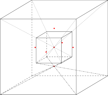
Figure 3.1. A representation of the $24$-cell. Vertex $\boldsymbol{H}$ is at infinity.