Low-Complexity Structured Precoding for Spatially Correlated MIMO Channels

Abstract

The focus of this paper is on spatial precoding in correlated multi-antenna channels, where the number of independent data-streams is adapted to trade-off the data-rate with the transmitter complexity. Towards the goal of a low-complexity implementation, a structured precoder is proposed, where the precoder matrix evolves fairly slowly at a rate comparable with the statistical evolution of the channel. Here, the eigenvectors of the precoder matrix correspond to the dominant eigenvectors of the transmit covariance matrix, whereas the power allocation across the modes is fixed, known at both the ends, and is of low-complexity. A particular case of the proposed scheme (semiunitary precoding), where the spatial modes are excited with equal power, is shown to be near-optimal in matched channels. A matched channel is one where the dominant eigenvalues of the transmit covariance matrix are well-conditioned and their number equals the number of independent data-streams, and the receive covariance matrix is also well-conditioned. In mismatched channels, where the above conditions are not met, it is shown that the loss in performance with semiunitary precoding when compared with a perfect channel information benchmark is substantial. This loss needs to be mitigated via limited feedback techniques that provide partial channel information to the transmitter. More importantly, we develop matching metrics that capture the degree of matching of a channel to the precoder structure continuously, and allow ordering two matrix channels in terms of their mutual information or error probability performance.

I Introduction

Multiple antenna communications has received significant attention over the last decade as a mechanism to increase the rate of information transfer, or the reliability of signal reception, or a combination of the two. The focus of this work is on point-to-point spatial precoding systems, where the number of independent data-streams is constrained to be a subset, $M$, of the transmit dimension so as to minimize the complexity and the cost associated with transmission. Initial works on precoding study optimal signaling strategies when perfect channel state information (CSI) is available at the transmitter and the receiver. These studies show that a channel diagonalizing input that corresponds to exciting the dominant $M$-dimensional eigen-space of the channel, with a power allocation that can be computed via waterfilling, is robust under different design metrics [1, 2, 3, 4, 5, 6, 7, 8, 9].

Although perfect CSI provides a benchmark on the performance, it is difficult to obtain in practice. More importantly, the system performance is not robust under CSI uncertainty. Even a small error in the CSI at the transmitter can lead to a dramatic degradation in performance with a scheme that is designed for the mismatched CSI [10, 11, 12, 13, 14]. Furthermore, even if perfect CSI is available, tight constraints on complexity as well as energy consumption [15, 16, 17, 18, 19] at the RF level in the mobile ends may disallow the implementation of optimal solutions in practice. This is because Third Generation wireless systems and beyond are expected to be multi-carrier in nature and the burden of computing the optimal input is magnified by the number of sub-carriers and the rate of evolution of the channel realizations. Besides this, the structure of the input could change, often dramatically, at the rate of evolution of the channel realizations, which also makes it difficult to implement. These reasons suggest that a slower rate of adaptation of the input signals, that is of low complexity and is more robust to CSI uncertainty, is preferred in practice.

In realistic wireless systems, where the channels are spatio-temporally correlated, the slow rate of statistical evolution implies that it is reasonable to assume perfect statistical knowledge of the channel at the transmitter. Since the spatial statistics experienced by the individual sub-carriers are identical [20, 21, 22], the burden of computing the optimal input with only the statistical information at the transmitter is equivalent to that of a narrowband system. Even in this setting, optimal precoding has been studied for different spatial correlation models [23, 24, 25, 26, 27, 21, 28, 10, 11, 29, 30, 31, 32]. These works show that the eigen-directions of the optimal input covariance matrix correspond to a set of the $M$-dominant eigenvectors of the transmit covariance matrix and are hence, easily adaptable to changes in statistics. However, computing the power allocation across the $M$ modes requires Monte Carlo averaging or gradient descent-type approaches [21, 28, 10, 11, 29]. While the computational complexity of the power allocation algorithm may be affordable at the base station end, whether it is possible or not at the mobile end is questionable. Moreover, there has been no systematic study of statistics-based precoding approaches and hence, it is not clear as to how far the performance of the statistical scheme is with respect to the perfect CSI benchmark.

It should be noted that all the above works study precoder design with an emphasis on obtaining information-theoretic limits on performance. In contrast, our focus here is on low-complexity schemes that can be easily implemented and easily adapted to changes in channel statistics. In this work, we consider a narrowband setup where spatial correlation is modeled by a general decomposition [33, 28, 34] that: 1) Is based on physical principles, 2) Has been verified by many recent measurement campaigns, and 3) Includes as special cases the well-studied i.i.d. model, the separable correlation model [35], and the virtual representation [36, 21, 20].

We propose the notion of structured precoding, where the power allocation across the $M$ spatial modes is fixed and known at both the ends. Two specific cases are studied in depth in this work: 1) A statistical semiunitary precoder, where the eigen-directions of the input correspond to the dominant eigenvectors of the transmit covariance matrix and the power allocation is uniform, is studied theoretically. 2) A precoder, where the eigen-directions are as before, and the power is allocated proportionate to the transmit covariance matrix eigenvalues below a threshold signal-to-noise ratio (${\sf{SNR}}$) and uniformly above this ${\sf{SNR}}$, is studied via simulations. Following the philosophy propounded here, more complicated schemes, where the power allocation across the modes can be computed with low-complexity, possibly as a function of the ${\sf{SNR}}$ and the statistics, can also be considered.

Our focus is on two questions: 1) When is the first scheme near-optimal with respect to a perfect CSI benchmark?, and 2) What is the “gap” in performance and how does it depend on the system and the channel parameters? The performance metric used in this work is relative average mutual information loss. We also study relative uncoded error probability enhancement and relative mean-squared error (${\sf{MSE}}$) enhancement, whenever they can be characterized analytically.

The answers to the above questions lie in the notion of matched and mismatched channels, which are introduced in this work. A matched channel is one where the channel is effectively matched to the precoding scheme with the following two conditioning properties being true: 1) The $M$-dominant eigenvalues of the transmit covariance matrix are well-conditioned, whereas the remaining $(N_{t}-M)$ eigenvalues are ill-conditioned away from the dominant ones, and 2) The receive covariance matrix is also well-conditioned. A mismatched channel is one where both the transmit and the receive covariance matrices are ill-conditioned, with the additional condition that ${\sf rank}({\bf H})\geq M$ with probability $1$.

We show that matched and mismatched channels correspond to the cases where the relative performance of the semiunitary precoder are closest and farthest to the perfect CSI precoder, respectively. The degree of channel-to-precoder scheme matching can be abstractly measured with matching metrics, that are also introduced in this work. As a by-product of our study, we also show that the semiunitary precoder is near-optimal in the relative antenna asymptotic setting for any channel. This paper generalizes previous work [14] on the beamforming case ($M=1$), where we studied the performance of the statistical beamforming scheme.

Organization: After elucidating the system model in Section II, we benchmark the structure of the optimal structured precoder in the perfect CSI case in Section III. Using tools from majorization theory, we show that the optimal input naturally extends the channel-diagonalizing input from the unconstrained case [1, 2, 3, 4, 5, 6, 7, 8, 9]. In Section IV, we elaborate on the problem setup of structured precoding. In Sections V-VII, using tools from random matrix theory and eigenvector perturbation theory, we study the asymptotic (in antenna dimensions) performance of a statistical semiunitary precoder that excites the $M$-dominant eigenvectors of the transmit covariance matrix. We provide numerical studies to illustrate the benefits of the proposed precoding scheme under realistic system assumptions in Section VIII with a discussion of our results and conclusions in Section IX. Proofs of most of the claims have been relegated to the appendices.

Notation: The $M$-dimensional identity matrix is denoted by ${{\mathbf{I}}}_{M}$. The $i,j$-th and $i$-th diagonal entries of a matrix ${\mathbf{X}}$ are denoted by ${\mathbf{X}}(i,j)$ and ${\mathbf{X}}(i)$, respectively. In more complicated settings (for example, when the matrix ${\mathbf{X}}$ is represented as a product or sum of many matrices), the above entries are denoted by ${\mathbf{X}}_{ij}$ and ${\mathbf{X}}_{i}$, respectively. The complex conjugate, conjugate transpose, regular transpose and inverse operations are denoted by $(\cdot)^{\star}$, $(\cdot)^{H}$, $(\cdot)^{T}$ and $(\cdot)^{-1}$ while the expectation, the trace and the determinant operators are given by ${\mathit{E}}[\cdot]$, ${\mathrm{Tr}}(\cdot)$ and $\det(\cdot)$, respectively. The $t$-dimensional complex vector space is denoted by ${\mathbb{C}}^{t}$. The standard big-Oh (${\mathcal{O}}$) and small-oh (${\mathnormal{o}}$) notations are used along with the standard ordering for eigenvalues of an $n\times n$-dimensional Hermitian matrix ${\mathbf{X}}$: $\lambda_{1}({\mathbf{X}})\geq\cdots\geq\lambda_{n}({\mathbf{X}})$. The largest and the smallest eigenvalues are often denoted also by $\lambda_{\max}({\mathbf{X}})$ and $\lambda_{\min}({\mathbf{X}})$, respectively. The notation $x^{+}$ stands for $\max(x,0)$.

II System Setup

We consider a communication model with $N_{t}$ transmit and $N_{r}$ receive antennas, where $M$ ($1\leq M\leq N_{t}$) independent data-streams are used in signaling. That is, the $M$-dimensional input vector ${\bf s}$ is precoded into an $N_{t}$-dimensional vector via the $N_{t}\times M$ precoding matrix ${\bf F}$ and transmitted over the channel. The discrete-time baseband signal model used is

$${\mathbf{y}}={\bf H}\hskip 1.4457pt{\bf F}\hskip 1.4457pt{\bf s}+{\bf n},$$ (1)

where ${\mathbf{y}}$ is the $N_{r}$-dimensional received vector, ${\bf H}$ is the $N_{r}\times N_{t}$-dimensional channel matrix, and ${\bf n}$ is the $N_{r}$-dimensional (zero mean, unit variance) additive white Gaussian noise. In practice, the choice of $M$ is decided based on a trade-off between complexity, cost and performance gain.

II-A Channel Model

The main emphasis of this work is on the impact of spatial correlation. We isolate the spatial aspect by assuming a block fading, narrowband model for the time-frequency correlation of ${\bf H}$. It is well-known that Rayleigh fading (zero mean complex Gaussian) is an accurate model for ${\mathbf{H}}$ in a non line-of-sight setting and hence, the complete spatial statistics are described by the second-order moments of $\{{\mathbf{H}}(i,j)\}$.

The most general, mathematically tractable spatial correlation model is a canonical decomposition of the channel along the transmit and the receive covariance bases [33, 28, 34]. In this model, we assume that the auto- and the cross-covariance matrices of all rows of ${\bf H}$ have the same eigen-basis (denoted by ${\bf U}_{t}$), and the auto- and the cross-covariance matrices of all the columns of ${\bf H}$ have the same eigen-basis (denoted by ${\bf U}_{r}$). Thus, we can decompose ${\bf H}$ as

$${\mathbf{H}}={\mathbf{U}}_{r}\hskip 1.4457pt{\mathbf{H}}_{{\sf{ind}}}\hskip 1.4457pt{\mathbf{U}}_{t}^{\sl H},$$ (2)

where ${\mathbf{H}}_{{\sf{ind}}}$ has independent, but not necessarily identically distributed entries, and ${\mathbf{U}}_{t}$ and ${\mathbf{U}}_{r}$ are unitary matrices. The transmit and the receive covariance matrices are defined as

$${\mathbf{\Sigma}}_{t}\triangleq{\mathit{E}}[{\mathbf{H}}^{H}{\mathbf{H}}] = {\mathbf{U}}_{t}\hskip 1.4457pt{\mathit{E}}[{\mathbf{H}}_{{\sf{ind}}}^{H}{\mathbf{H}}_{{\sf{ind}}}]\hskip 1.4457pt{\mathbf{U}}_{t}^{\sl H}={\mathbf{U}}_{t}{\mathbf{\Lambda}}_{t}{\mathbf{U}}_{t}^{\sl H},$$ (3)

$${\mathbf{\Sigma}}_{r}\triangleq{\mathit{E}}[{\mathbf{H}}{\mathbf{H}}^{H}] = {\mathbf{U}}_{r}\hskip 1.4457pt{\mathit{E}}[{\mathbf{H}}_{{\sf{ind}}}{\mathbf{H}}_{{\sf{ind}}}^{H}]\hskip 1.4457pt{\mathbf{U}}_{r}^{\sl H}={\mathbf{U}}_{r}\hskip 1.4457pt{\mathbf{\Lambda}}_{r}\hskip 1.4457pt{\mathbf{U}}_{r}^{\sl H},$$ (4)

where ${\mathbf{\Lambda}}_{t}={\mathit{E}}[{\mathbf{H}}_{{\sf{ind}}}^{H}{\mathbf{H}}_{{\sf{ind}}}]$ and ${\mathbf{\Lambda}}_{r}={\mathit{E}}[{\mathbf{H}}_{{\sf{ind}}}{\mathbf{H}}_{{\sf{ind}}}^{H}]$ are diagonal.

Under certain special cases, the model in (2) reduces to some well-known spatial correlation models such as the i.i.d. model, the separable correlation [35] and the virtual representation [36, 21, 20] frameworks. The readers are referred to [13] for details. The i.i.d. model, while being analytically tractable, is unrealistic for applications where large antenna spacings or a rich scattering environment are not possible. Even though the separable model may be an accurate fit under certain channel conditions [38], deficiencies acquired by the separability property result in misleading estimates of system performance [39, 40, 34]. The readers are referred to [39, 33, 41] for more details on how the canonical, and more specifically the virtual model fit measured data better. Given a correlated channel, in this work, we will assume without any loss in generality that $M\leq{\sf rank}({\bf\Lambda}_{t})\leq N_{t}.$

II-B Channel State Information

Initial works in the precoding literature have assumed perfect CSI at both the transmitter and the receiver. Perfect CSI at the receiver (the coherent case) is usually reasonable for systems that adopt a ‘training followed by signaling’ model. On the other hand, both the perfect and the no CSI assumptions at the transmitter are unrealistic, being too optimistic and too pessimistic, respectively. This is so because the perfect CSI condition imposes a huge burden on the training or the feedback apparatus on the reverse link while on the other hand, the spatial statistics of the channel entries evolve over much slower timescales and can be learned at both the ends. In this work, we study the coherent case with perfect statistical knowledge at the transmitter.

II-C Transceiver Architecture

The transmitted vector ${\bf F}{\bf s}$ (see (1)) has a power constraint $\rho$. The transmit power constraint can be rewritten as

$$\rho={\mathit{E}}\left[{\bf s}^{H}\hskip 1.4457pt{\bf F}^{H}\hskip 1.4457pt{\bf F}\hskip 1.4457pt{\bf s}\right]={\mathrm{Tr}}\left({\mathit{E}}\left[{\bf F}\hskip 1.4457pt{\bf s}\hskip 1.4457pt{\bf s}^{H}\hskip 1.4457pt{\bf F}^{H}\right]\right)={\mathrm{Tr}}\left({\bf F}\hskip 1.4457pt{\mathbf{Q}}_{s}\hskip 1.4457pt{\bf F}^{H}\right),\hskip 7.22743pt{\mathbf{Q}}_{s}\triangleq{\mathit{E}}\left[{\bf s}\hskip 1.4457pt{\bf s}^{H}\right].$$ (5)

By decomposing ${\bf F}$ and ${\mathbf{Q}}_{s}$ using singular value decomposition (SVD) and renormalizing, it can be seen that the system equation can be written as:

$${\mathbf{y}} = {\bf H}\hskip 1.4457pt{\bf F}\hskip 1.4457pt{\bf s}+{\bf n},\hskip 7.22743pt{\bf F}=\sqrt{\frac{\rho}{M}}\hskip 1.4457pt{\bf V}_{{\bf F}}\hskip 1.4457pt{{\mathbf{\Lambda}}}_{{\bf F}}^{1/2},$$ (6)

where ${\bf V}_{{\bf F}}$ is an $N_{t}\times M$ semiunitary matrix, ${{\mathbf{\Lambda}}}_{{\bf F}}$ is an $M\times M$ non-negative definite power shaping (allocation) matrix with ${\mathrm{Tr}}({\mathbf{\Lambda}}_{{\bf F}})\leq M$, and ${\bf s}$ is an $M\times 1$ vector with i.i.d. components that have zero mean and variance one. That is, the general precoder can be thought of as a power loading by ${\mathbf{\Lambda}}_{{\bf{F}}}$, followed by a rotation with ${\bf V}_{{\bf{F}}}$.

The optimal reception strategy of the input symbols corresponds to non-linear maximum likelihood (ML) decoding. However, the exponential complexity of ML decoding in both antenna dimensions and coherence length implies that simpler receiver architectures are preferred. In this work, we assume a linear minimum mean-squared error (${\sf MMSE}$) receiver. With this receiver, the symbol corresponding to the $k$-th data-stream is recovered by projecting the received signal ${\bf y}$ on to the $N_{r}\times 1$ vector

$${\bf g}_{k} = \sqrt{\frac{\rho}{M}}\left(\frac{\rho}{M}{\mathbf{H}}{\bf F}{\bf F}^{H}{\bf H}^{H}+{\bf I}_{N_{r}}\right)^{-1}{\bf H}{\bf f}_{k},$$ (7)

where ${\bf f}_{k}$ is the $k$-th column of ${\bf F}$. That is, the recovered symbol is $\widehat{{\bf s}}(k)={\bf g}_{k}^{H}{\bf y}$, and the signal-to-interference-noise ratio (${\sf{SINR}}$) at the output of the linear filter ${\bf g}_{k}$ is

$${\sf{SINR}}_{k}=\frac{1}{\left[\left({{\mathbf{I}}}_{M}+\frac{\rho}{M}{\bf F}^{\sl H}{\bf H}^{\sl H}{\bf H}{\bf F}\right)^{-1}\right]_{k}}-1.$$ (8)

Also, note that the ${\sf{MSE}}$ of the $k$-th data-stream, ${\sf{MSE}}_{k}$, is given by $\left[\left({{\mathbf{I}}}_{M}+\frac{\rho}{M}{\bf F}^{\sl H}{\bf H}^{\sl H}{\bf H}{\bf F}\right)^{-1}\right]_{k}$.

II-D A Case for Structured Precoding

Almost all of the current works on precoder design do not assume any specific structure on the precoder matrix ${\bf F}$. This is because the main focus of these works is on characterizing the fundamental performance limits of precoding. That is, to study optimal signaling schemes from a mutual information or an error probability viewpoint.

The structure of the optimal precoder, ${\bf F}_{{\sf{opt}}}$, critically depends on the knowledge of the eigenspace of ${\mathbf{H}}$ (see Sec. III). Even a small inaccuracy in the knowledge of the eigenspace of ${\mathbf{H}}$ could lead to a precoder with a significantly degraded performance [10, 11, 12, 13, 14]. While this issue does not arise in the perfect CSI case, it is critical in systems with imperfect CSI. In particular, imperfect channel knowledge arises in practice due to constraints on the quality and frequency of channel or statistical feedback and channel estimation at the receiver.

Moreover, even if perfect CSI is available at the transmitter, the efficient utilization of this information is constrained by fundamental limits on energy per bit constraints at the computational or processing level [15, 16, 17, 18, 19]. These limits in turn imply that a large number of computations are difficult to realize in low-power devices, such as those found at the mobile ends. For example, the move towards multi-carrier signaling and the fast rate at which channel realizations evolve leads to computational limits on how many SVD operations can be afforded. Another key aspect to note is that the eigenspace of the optimal input could change dramatically from one channel realization to the next, and this poses constraints on the adaptivity of the solutions proposed in the literature. In fact, RF design constraints imposed by the above limits are often the principal stumbling blocks in realizing multi-antenna systems in practice. The readers are referred to [18] for a broad array of RF design challenges, imposed by computational and complexity constraints.

All of the above reasons suggest that it may not be possible for ${\bf F}$ to be designed at an arbitrarily fast rate. They also suggest that ${\bf F}$ cannot have arbitrary structure and one cannot learn it with arbitrarily fine precision. The case of statistical precoding, where the optimal input is adapted in response to the statistical information has thus received significant attention. In this case, computing the optimal power allocation across the excited modes requires either Monte Carlo averaging or gradient descent-type approaches (see Sec. IV). The affordability of the complexity of these approaches at the mobile end is again questionable.

These reasons motivate us to study structured precoding, where the eigen-modes as well as the power allocation across them are determined via low-complexity operations on the channel statistics. The additional structure imposed on ${\bf F}$ serves the following purposes: 1) Isolating the impact of inaccuracy in the singular vectors and singular values of ${\bf F}$ on performance with respect to a genie-aided design, 2) Given that there are resource constraints on the reverse link quantization, identifying those features of the channel ${\bf H}$ that require an appropriate resource allocation so as to optimize system performance, and 3) Obtaining more realistic ‘intermediate’ benchmarks for systems in practice.

We first focus on a specific class of semiunitary precoder, where ${\bf\Lambda}_{\bf F}={\mathbf{I}}_{M}$. We then consider the more general structured precoder case, where ${\bf\Lambda}_{{\bf F}}$ is fixed, but is chosen different from the identity matrix.

III Perfect CSI Benchmark for Structured Precoding

Towards the eventual goal of studying a structured statistical precoding scheme, we first characterize the optimal perfect CSI benchmark in this section.

III-A Unconstrained Precoders

If only one data-stream is excited ($M=1$), the received ${\sf{SNR}}$ is given by $\rho\hskip 1.4457pt\frac{|{\bf z}^{H}{\bf H}{\bf f}|^{2}}{{\bf z}^{H}{\bf z}}$, where ${\bf f}$ is the beamforming vector and ${\bf z}$ is the combining vector. It is straightforward to note that the jointly optimal design of ${\bf z}$ and ${\bf f}$ can be reduced to a beamformer design by using the combining vector $\frac{{\bf H}{\bf f}}{\sqrt{{\bf f}^{H}{\bf H}^{H}{\bf H}{\bf f}}}$, and that the optimal choices ${\bf f}_{{\sf{opt}}}$ and ${\bf z}_{{\sf{opt}}}$ are the dominant right singular vector of ${\bf H}$ and $\frac{{\bf H}{\bf f}_{{\sf{opt}}}}{\sqrt{\lambda_{\max}({\bf H}^{H}{\bf H})}}$, respectively [42]. In this case, the received ${\sf{SNR}}$ coincides with $\rho\hskip 3.61371pt\lambda_{\max}({\bf H}^{H}{\bf H})$.

In contrast to beamforming, the precoding case with $M>1$ requires a recourse to the study of eigenvalues of products of Hermitian matrices. For the (general) unconstrained precoding case, the joint precoder-equalizer design turns out to have a channel diagonalizing structure. To state this result, we need some additional notation. Let an SVD of ${\bf H}$ be given by ${\bf H}={\bf U}_{\bf H}{\bf\Lambda}_{\bf H}{\bf V}_{\bf H}^{\sl H}$, where ${\bf V}_{\bf H}=[{\bf v}_{1}\cdots{\bf v}_{N_{t}}]$. Without any loss in generality, we assume that the non-trivial singular values of ${\bf H}$ are arranged in the standard order.

Lemma 1

The optimal choice of ${\bf V}_{{\bf F}_{{\sf{opt}}}}$ and ${\bf\Lambda}_{{\bf F}_{{\sf{opt}}}}$ in (6) are as follows: ${\bf V}_{{\bf F}_{{\sf{opt}}}}$ corresponds to $[{\bf v}_{1}\cdots{\bf v}_{M}]$, and the diagonal entries of ${\mathbf{\Lambda}}_{{\bf F}_{{\sf{opt}}}}$ are obtained via waterfilling.

Proof:

The optimality of the channel diagonalizing structure has been proved in [1, 2, 3, 4], with the design metric being the average ${\sf{MSE}}$ of the data-streams. Other design metrics where the channel diagonalizing structure is optimal include weighted ${\sf{MSE}}$ of the data-streams [5, 6], determinant of the ${\sf{MSE}}$ matrix [7], and a peak-power constraint metric [8]. A unified convex programming framework for precoder optimization is proposed in [9] by studying two broad classes of functions: Schur-concave and Schur-convex functions. In [9], the authors show that most of the above design criteria can be formulated as either a Schur-concave or Schur-convex function of the ${\sf{MSE}}$ and the channel diagonalizing structure is optimal in either case. ∎

III-B Semiunitary Precoders

When the precoders are constrained to be structured, it is intuitive (but not obvious) to expect a channel diagonalizing structure to be optimal. The following series of propositions elucidate the optimality of this structure in the semiunitary case with certain restrictions on the objective function. The more general structured case will be considered thereafter. The readers are referred to App. -A for many relevant definitions and results from majorization theory. Following the introduction from App. -A, we are prepared for the following.

III-B1 Precoders that Optimize Schur-concave Objective Functions

Proposition 1

Let $f:{\mathbb{R}}^{M}\mapsto{\mathbb{R}}$ be a Schur-concave function over its domain. Also, let $f(\cdot)$ be monotonically increasing in its arguments. That is, let the univariate function $f(\cdots,x_{k},\cdots):{\mathbb{R}}\mapsto{\mathbb{R}}$ be monotonically increasing for all $k$. If ${\sf{MSE}}=[{\sf{MSE}}_{1}\hskip 3.61371pt\cdots\hskip 3.61371pt{\sf{MSE}}_{M}]$, then the optimal choice of semiunitary precoder ${\bf F}_{{\sf{opt}}}$ that minimizes $f({\sf{MSE}})$ is given by

$${\bf F}_{{\sf{opt}}}=[{\mathbf{v}}_{1}\hskip 1.4457pt\cdots\hskip 1.4457pt{\mathbf{v}}_{M}].$$ (9)

Proof:

See Appendix -B. ∎

The utility of the above proposition can be gauged from the fact that a large class of useful functions satisfy the Schur-concavity property. For example, from Remark 2 in App. -A, we see that any weighted arithmetic or geometric mean of $\{{\sf{MSE}}_{k}\}$ (with weights chosen appropriately) is Schur-concave. The same remark illustrates the limitations of this partitioning because the mutual information function cannot (in general) be expressed as a Schur-concave (or a Schur-convex) function of ${\sf{MSE}}$.

In the special case of Gaussian inputs, the objective function $f(\cdot)$ to be maximized is

$$f(\cdot)=\log\det\left({\mathbf{I}}_{M}+\frac{\rho}{M}{\bf F}^{H}{\bf H}^{H}{\bf H}{\bf F}\right)=-\log\det\left({\bf E}\right),$$ (10)

where ${\bf E}$ is the mean-squared error matrix defined as

$${\mathit{E}}[({\bf s}-\widehat{{\bf s}})({\bf s}-\widehat{{\bf s}})^{H}]\triangleq\left({\mathbf{I}}_{M}+\frac{\rho}{M}{\bf F}^{H}{\bf H}^{H}{\bf H}{\bf F}\right)^{-1}.$$ (11)

It can be shown that maximizing the mutual information with the Gaussian input (or alternately, minimizing the determinant of ${\bf E}$) can be easily accommodated in the framework of Prop. 1; see [9] for details. Alternately, an easy consequence of Lemma 10 (see App. -A) is the fact that a channel diagonalizing structure maximizes mutual information and this has been established in [43]. Also note that if $M=N_{t}$, any choice of ${\bf F}$ unitary leads to the same value of $f(\cdot)$. Extending the proof of [43] to the case of a non-Gaussian input requires closed-form expressions for the mutual information, which are (in general) difficult to obtain.

III-B2 Precoders that Minimize the Average Error Probability

Besides mutual information, uncoded error probability is another important metric that describes the performance of a communication system. We now show how the machinery of majorization theory can be used to study the error probability. We state the most general form of this study in the following proposition, with its particularization to the error probability case illustrated thereafter.

Proposition 2

Let $h:{\mathbb{R}}\mapsto{\mathbb{R}}$ be a continuous, increasing, and convex function of its argument. The optimal choice of ${\bf F}$ that minimizes $\sum_{k=1}^{M}h({\sf{MSE}}_{k})$ is given by

$${\bf F}_{{\sf{opt}}}=\left[{\mathbf{v}}_{1}\hskip 1.4457pt\cdots\hskip 1.4457pt{\mathbf{v}}_{M}\right]\hskip 1.4457pt{\mathbf{\Gamma}},$$ (12)

where ${\mathbf{\Gamma}}$ is an appropriately chosen unitary matrix (see App. -B for details on construction).

Proof:

See Appendix -B. ∎

If $h(\cdot)$ is as in Prop. 2, and $g:{\mathbb{R}}^{M}\mapsto{\mathbb{R}}$ is defined as

$$g({\sf{MSE}})\triangleq\sum_{k=1}^{M}h({\sf{MSE}}_{k}),$$ (13)

then it is important to note from Lemma 7 in App. -A that $g(\cdot)$ is a Schur-convex function of ${\sf{MSE}}$. Thus, in general, Prop. 2 is neither a consequence of nor implies Prop. 1.

We now show how Prop. 2 is useful in the error probability setting. Let $P_{{\sf{err}}}$ denote the probability that at least one of the $M$ data-streams is in error. Then,

$$P_{{\sf{err}}}=1-\prod_{k=1}^{M}(1-P_{k}),$$ (14)

where $P_{k}$ is the probability that the $k$-th data-stream is in error. If some fixed constellation is used for signaling across all the data-streams, we can write $P_{k}$ as

$$P_{k}=\alpha{\cal Q}\left(\beta\hskip 1.4457pt\big{(}{\sf{SINR}}_{k}\big{)}^{1/2}\right),$$ (15)

where ${\sf{SINR}}_{k}$ is the received ${\sf{SINR}}$ of the $k$-th data-stream after linear processing [44], $\alpha$ and $\beta$ are constants dependent only on the type of the constellation, and ${\cal Q}(\cdot)$ is the ${\cal Q}$-function associated with a standard Gaussian random variable. Assuming that the error probability of the weakest data-stream is sufficiently small (which is reasonable for most design problems), we have $P_{{\sf{err}}}\approx\sum_{k=1}^{M}P_{k}$. Alternately, one could consider a metric that measures the average error probability of the individual data-streams: $\frac{1}{M}\hskip 1.4457pt\sum_{k=1}^{M}P_{k}$. Thus, in either case, we are interested in studying the optimal choice of precoder ${\bf F}$ that minimizes $\sum_{k=1}^{M}P_{k}$.

It is straightforward to note that $P_{k}(\cdot)$ is a continuous and increasing function of ${\sf{MSE}}$. Besides, it is shown in [9] that $P_{k}(\cdot)$ is a convex function of ${\sf{MSE}}$ as long as the argument is sufficiently small. We are thus justified in assuming that $P_{k}(\cdot)$ is convex, continuous and increasing in ${\sf{MSE}}$. Then, Prop. 2 shows that $P_{{\sf{err}}}$ is minimized by ${\bf F}_{{\sf{opt}}}$ as in (12).

III-B3 Precoders that Optimize Schur-convex Objective Functions

It is natural to probe the optimality of ${\bf F}_{{\sf{opt}}}$ in (12) if instead of the average error probability, we considered the error probability corresponding to the weakest data-stream. For this, we now need the counterpart of Prop. 1 which is as follows.

Proposition 3

Let $f:{\mathbb{R}}^{M}\mapsto{\mathbb{R}}$ be a Schur-convex function over its domain. Also, let $f(\cdot)$ be monotonically increasing in its arguments. The optimal choice of semiunitary precoder ${\bf F}_{{\sf{opt}}}$ that minimizes $f({\sf{MSE}})$ is given by

$${\bf F}_{{\sf{opt}}}=[{\mathbf{v}}_{1}\hskip 1.4457pt\cdots\hskip 1.4457pt{\mathbf{v}}_{M}]\hskip 1.4457pt{\mathbf{\Gamma}},$$ (16)

where ${\mathbf{\Gamma}}$ is the same unitary matrix as defined in Prop. 2.

Proof:

The proof follows along the same lines as Prop. 2. No details are provided. ∎

To answer the question that led towards the above proposition, note from Lemma 8 in App. -A that $\max_{k}P_{k}$ is a Schur-convex function of ${\sf{MSE}}$. Thus from Prop. 3, the optimal precoder is as in (16). Further, note that the matrix ${\bf\Gamma}$ in the description of ${\bf F}_{{\sf{opt}}}$ in (12) and (16) can be ignored since ${\bf s}$ is i.i.d. and therefore, so is ${\bf\Gamma}{\bf s}$.

III-C General Structured Precoders

We now generalize our results to the general structured case.

Proposition 4

Let the structure of the precoder be ${\bf F}={\bf V}_{\bf F}\hskip 1.4457pt{\bf\Lambda}_{{\sf fixed}}^{1/2}$, where ${\bf\Lambda}_{{\sf fixed}}$ is some fixed matrix of rank $M$ with ${\mathrm{Tr}}({\bf\Lambda}_{{\sf fixed}})\leq M$, albeit chosen arbitrarily. That is, in the ensuing optimization ${\bf\Lambda}_{{\sf fixed}}$ is fixed and we only optimize over ${\bf V}_{\bf F}$. As before, the structure of the optimal ${\bf V}_{\bf F}$ depends on the nature of the objective function.

• Schur-concave objective functions (and in particular, the mutual information with Gaussian input) are optimized by ${\bf F}$ of the form:

  $${\bf F}_{{\sf{opt}}}=[{\mathbf{v}}_{1}\hskip 1.4457pt\cdots\hskip 1.4457pt{\mathbf{v}}_{M}]\hskip 3.61371pt{\bf\Lambda}_{{\sf fixed}}^{1/2}.$$ (17)

• Schur-convex objective functions (and in particular, the average uncoded error probability) are optimized by ${\bf F}$ of the form:

  $${\bf F}_{{\sf{opt}}}=[{\mathbf{v}}_{1}\hskip 1.4457pt\cdots\hskip 1.4457pt{\mathbf{v}}_{M}]\hskip 3.61371pt{\bf\Lambda}_{{\sf fixed}}^{1/2}\hskip 3.61371pt{\bf\Gamma}$$ (18)

  for an appropriately chosen unitary matrix ${\bf\Gamma}$.

Proof:

We follow the same proof techniques of Prop. 1-3. See Appendix -B for details. ∎

Thus, even in the more general structured precoding case, the channel diagonalizing structure is optimal.

IV Statistical Precoding: Preliminaries

We now assume that instantaneous channel information is not available at the transmitter, but channel statistics are known.

IV-A Notations

While much of the notations required in the rest of the paper have been established in Sec. II-A, we find it convenient to restate some of them that are often used in the ensuing sections. We assume that ${\bf H}$ is described by either the separable model or the more general non-separable model of (2). Let the variance of ${\bf H}_{{\sf{ind}}}(i,j)$ be denoted by $\sigma_{ij}^{2}$. The eigenvalues of the transmit covariance matrix are denoted by $\{{\bf\Lambda}_{t}(k)\}$ in the separable case while in the non-separable case, they are denoted by $\gamma_{t,k}\triangleq\sum_{i=1}^{N_{r}}\sigma_{ik}^{2}$. In either case, we assume that the columns of ${\mathbf{H}}_{{\sf{ind}}}$ are arranged such that the transmit eigenvalues are in decreasing order. The channel power of ${\bf H}$, $\rho_{c}$, is given by $\rho_{c}=\sum_{i=1}^{N_{r}}{\bf\Lambda}_{r}(i)=\sum_{i=1}^{N_{t}}{\bf\Lambda}_{t}(i)$. The normalized channel power is $\gamma_{r}\triangleq\frac{\rho_{c}}{N_{r}}$.

In the separable case, let ${\widetilde{{\mathbf{\Lambda}}}}_{t}$ denote the principal $M\times M$ sub-matrix of ${\mathbf{\Lambda}}_{t}$ and ${\bf\widetilde{H}}_{{\sf{iid}}}$ denote the $N_{r}\times M$ principal sub-matrix of ${\bf H}_{{\sf{iid}}}$. That is,

$${\bf H}_{{\sf{iid}}}=\left[\begin{array}[]{cc}\underbrace{{\bf\widetilde{H}}_{{\sf{iid}}}}_{N_{r}\times M}&\underbrace{\times}_{N_{r}\times(N_{t}-M)}\end{array}\right].$$ (20)

Without any explicit reference to $k$, we will often denote by ${\widehat{{\mathbf{\Lambda}}}}_{t}$, the $(M-1)\times(M-1)$ matrix obtained from ${\widetilde{{\mathbf{\Lambda}}}}_{t}$ by removing the $k$-th row and $k$-th column and by ${\bf\widehat{H}}_{{\sf{iid}}}$, the matrix obtained from ${\bf\widetilde{H}}_{{\sf{iid}}}$ by removing the $k$-th column alone. In the non-separable case, let $\widetilde{{\mathbf{H}}}_{{\sf{ind}}}$ denote the $N_{r}\times M$-dimensional principal sub-matrix of ${{\mathbf{H}}}_{{\sf{ind}}}$.

IV-B Unconstrained Precoders

Lemma 2

The optimal precoder ${\bf F}_{{\sf{stat}},\hskip 1.4457pt{\sf{opt}}}$ is of the form ${\bf V}_{{\sf{stat}}}\hskip 1.4457pt{\bf\Lambda}_{{\sf{stat}}}^{1/2}$, where ${\bf V}_{{\sf{stat}}}$ is a set of $M$ dominant eigenvectors of the transmit covariance matrix ${\bf\Sigma}_{t}$ and ${\bf\Lambda}_{{\sf{stat}}}$ is the unique solution to the following constrained optimization:

$${\bf\Lambda}_{{\sf{stat}}}=\arg\max_{{\bf\Lambda}\in{\cal L}}{\mathit{E}}_{{\mathbf{H}}}\left[\log\det\left({\mathbf{I}}_{N_{r}}+\frac{\rho}{M}\hskip 3.61371pt\widetilde{{\mathbf{H}}}_{{\sf{ind}}}\hskip 1.4457pt{\bf\Lambda}\hskip 1.4457pt{\widetilde{{\mathbf{H}}}}_{{\sf{ind}}}^{H}\right)\right]$$ (21)

with ${\cal L}=\{{\bf\Lambda}\}$ denoting the convex set of all diagonal $M\times M$ non-negative definite matrices such that ${\mathrm{Tr}}({\bf\Lambda})\leq M$.

The optimality of the dominant eigenvectors of ${\bf\Sigma}_{t}$ is not surprising (see [23, 24, 25, 26, 21, 28, 10, 11] and references therein for problems of a similar nature). The optimization in (21) is standard: Maximizing a concave function over a convex set. A gradient descent-type approach for this is provided in [30] and a Monte Carlo approach is provided in [21, 28, 29].

IV-C Structured Statistical Precoders

As explained in Sec. II-D, the complexity of solving for ${\bf\Lambda}_{{\sf{stat}}}$ in (21) may be unaffordable in many practical scenarios. We therefore pursue two statistics-based precoders: ${\bf F}_{{\sf semi}}$ and ${\bf F}_{{\sf fixed}}$, with ${\bf F}_{{\sf semi}}={\bf V}_{{\sf{stat}}}$ and ${\bf F}_{{\sf fixed}}={\bf V}_{{\sf{stat}}}\hskip 1.4457pt{\bf\Lambda}_{{\sf fixed}}^{1/2}$. The choice of ${\bf\Lambda}_{{\sf fixed}}$ that is of interest here is:

$${\bf\Lambda}_{{\sf fixed}}(k)=\left\{\begin{array}[]{cc}M\cdot\frac{{\bf\Lambda}_{t}(k)}{\sum_{j=1}^{M}{\bf\Lambda}_{t}(j)}&{\rm if}\hskip 3.61371pt\rho<{\sf{SNR}}_{\sf T},\\ 1&{\rm if}\hskip 3.61371pt\rho\geq{\sf{SNR}}_{\sf T}.\end{array}\right.$$ (24)

The threshold ${\sf{SNR}}$ (${\sf{SNR}}_{\sf T}$) is such that

$${\sf{SNR}}_{\sf T}=\alpha\frac{M}{{\bf\Lambda}_{t}(M)}$$ (25)

for an appropriate choice of $\alpha,\alpha>1$. This choice is motivated by our recent work [45] on transient-${\sf{SNR}}$ (the ${\sf{SNR}}$ at which exciting $M$ modes is information theoretically optimal) design.

For a given channel realization, let $I_{{\sf{stat}},\hskip 1.4457pt{\sf semi}}(\rho)$ and $P_{{\sf{err}},\hskip 1.4457pt{\sf{stat}},\hskip 1.4457pt{\sf semi}}(\rho)$ denote the mutual information and error probability achievable with ${\bf F}_{{\sf semi}}$, while $I_{{\sf{stat}},\hskip 1.4457pt{\sf fixed}}(\rho)$ and $P_{{\sf{err}},\hskip 1.4457pt{\sf{stat}},\hskip 1.4457pt{\sf fixed}}(\rho)$ denote the corresponding quantities with ${\bf F}_{{\sf fixed}}$, all at an ${\sf{SNR}}$ of $\rho$. Similarly, denote the corresponding quantities with the three perfect CSI precoders described in Lemma 1, (9) and (17) by: $I_{{\sf{perf}},\hskip 1.4457pt{\sf unconst}}(\rho)$, $I_{{\sf{perf}},\hskip 1.4457pt{\sf semi}}(\rho)$, $I_{{\sf{perf}},\hskip 1.4457pt{\sf fixed}}(\rho)$, and $P_{{\sf{err}},\hskip 1.4457pt{\sf{perf}},\hskip 1.4457pt{\sf unconst}}(\rho)$, $P_{{\sf{err}},\hskip 1.4457pt{\sf{perf}},\hskip 1.4457pt{\sf semi}}(\rho)$, $P_{{\sf{err}},\hskip 1.4457pt{\sf{perf}},\hskip 1.4457pt{\sf fixed}}(\rho)$, respectively. It is important to note the distinction between these quantities. While $I_{{\sf{stat}},\hskip 1.4457pt\bullet}(\rho)$ and $P_{{\sf{err}},\hskip 1.4457pt{\sf{stat}},\hskip 1.4457pt\bullet}(\rho)$ are functions of the channel realization ${\bf H}$, the precoder structure itself is independent of ${\bf H}$, but only dependent on the channel statistics. On the other hand, $I_{{\sf{perf}},\hskip 1.4457pt\bullet}(\rho)$ and $P_{{\sf{err}},\hskip 1.4457pt{\sf{perf}},\hskip 1.4457pt\bullet}(\rho)$ in addition to being dependent on the channel realization also correspond to precoders whose structure is dependent on ${\bf H}$ and chosen optimally.

IV-D Average Relative Difference Metrics

Towards the goal of studying the proposed scheme(s), we develop universal metrics that capture the performance gap between the proposed precoder(s) and an ideal benchmark. We first motivate the choice of our metric in an abstract context.

Let ‘scheme $1$’ and ‘scheme $2$’ denote two signaling schemes with $I_{{\sf scheme},\hskip 1.4457pt1}(\rho)$ and $I_{{\sf scheme},\hskip 1.4457pt2}(\rho)$ denoting the mutual information of the two schemes at an ${\sf{SNR}},\rho$. Our goal is to quantify whether scheme $1$ is better than scheme $2$ or not, and if so, by how much. For any signaling scheme, the average mutual information is a function of $\rho$ as well as the statistical description of the channel. Irrespective of the spatial correlation, the average mutual information of any scheme tends to zero as $\rho\rightarrow 0$ and tends to infinity as $\rho\rightarrow\infty$. For this reason, the difference in average mutual information between the two schemes can converge to zero as $\rho\rightarrow 0$ at a rate different from that of either scheme, and could blow up to infinity as $\rho\rightarrow\infty$. Thus, the difference in average mutual information is not a good measure for comparing the two schemes.

An efficient comparison of the two schemes is possible by using either of the following set of average relative difference metrics:

$$\Delta I_{{\rm scheme}\hskip 1.4457pt1,\hskip 3.61371pt{\rm scheme}\hskip 1.4457pt2} \triangleq \frac{{\mathit{E}}_{{\mathbf{H}}}\left[I_{{\sf scheme},\hskip 1.4457pt1}(\rho)-I_{{\sf scheme},\hskip 1.4457pt2}(\rho)\right]}{{\mathit{E}}_{{\mathbf{H}}}[I_{{\sf scheme},\hskip 1.4457pt2}(\rho)]},$$ (26)

$$\widetilde{\Delta I}_{{\rm scheme}\hskip 1.4457pt1,\hskip 3.61371pt{\rm scheme}\hskip 1.4457pt2} \triangleq {\mathit{E}}_{{\mathbf{H}}}\left[\frac{I_{{\sf scheme},\hskip 1.4457pt1}(\rho)-I_{{\sf scheme},\hskip 1.4457pt2}(\rho)}{I_{{\sf scheme},\hskip 1.4457pt2}(\rho)}\right].$$ (27)

Note that the choice of scheme $2$ in the denominator of (26) and (27) is the scheme that performs relatively poorly. Thus, $\Delta I_{\bullet}$ and $\widetilde{\Delta I}_{\bullet}$ correspond to a worst-case measure of relative performance. The metrics are more meaningful (than the difference metric) in studying the relative gap (or closeness) between the schemes, independent of the ${\sf{SNR}}$. While we have used the case of average mutual information to motivate the need for a relative difference metric, the same argument is applicable in the error probability case. In fact, the need for such a metric is more critical in the error probability case since the error probabilities of the schemes that are being compared (and hence, the difference between them) are small.

IV-E Problem Setup

The main goal of this paper is to quantify, as a function of the statistics and antenna dimensions,

$$\Delta I_{{\sf semi}} \triangleq \frac{{\mathit{E}}_{{\mathbf{H}}}\left[I_{{\sf{perf}},\hskip 1.4457pt{\sf unconst}}(\rho)-I_{{\sf{stat}},\hskip 1.4457pt{\sf semi}}(\rho)\right]}{{\mathit{E}}_{{\mathbf{H}}}\left[I_{{\sf{stat}},\hskip 1.4457pt{\sf semi}}(\rho)\right]}$$ (28)

in the case of mutual information, and

$$\Delta P_{{\sf semi}} \triangleq {\mathit{E}}_{{\mathbf{H}}}\left[\frac{P_{{\sf{err}},\hskip 1.4457pt{\sf{stat}},\hskip 1.4457pt{\sf semi}}(\rho)-P_{{\sf{err}},\hskip 1.4457pt{\sf{perf}},\hskip 1.4457pt{\sf unconst}}(\rho)}{P_{{\sf{err}},\hskip 1.4457pt{\sf{perf}},\hskip 1.4457pt{\sf unconst}}(\rho)}\right]$$ (29)

in the case of error probability. In addition, we are also interested in the corresponding quantities for ${\bf F}_{\sf fixed}$ in (24): $\Delta I_{\sf fixed}$ and $\Delta P_{\sf fixed}$.

While closed-form expressions for the above metrics seem difficult to obtain across all ${\sf{SNR}}$ regimes, the following simplifying assumptions render these metrics theoretically tractable.

• Asymptotics of Antenna Dimension(s): Any performance metric computation in the spatially correlated, finite antenna setting suffers from fundamental difficulties associated with a lack of knowledge of the joint probability density function of singular values of the channel matrix. However, under many settings, in the asymptotics of antenna dimension(s), the density function of eigenvalues converges (in an appropriate sense) to a certain deterministic density function. Many recent works on multi-antenna channels (see [21, 28, 10, 11] and references therein) exploit this fundamental property in the characterization of various information theoretic quantities of interest.

  In this work, we find it useful to separate our study into two cases: 1) An easily tractable case of relative receive antenna asymptotics, where $\frac{M}{N_{r}}\rightarrow 0$, and 2) A more difficult case of proportional growth of antenna dimensions, where both $\{M,N_{r}\}\rightarrow\infty$ with $\frac{M}{N_{r}}\rightarrow\gamma$ and $\gamma\in(0,\infty)$ is a constant. The first case includes the following sub-cases in a unified way: a) $N_{t}$ and $M$ are finite and $N_{r}\rightarrow\infty$, b) $\big{\{}M,N_{r}\big{\}}\rightarrow\infty$ with $\frac{M}{N_{r}}\rightarrow 0$, and c) via a relabeling of indices the case where $\frac{M}{N_{r}}\rightarrow\infty$ with either $N_{r}$ finite or $N_{r}\rightarrow\infty$.

• Signaling Constellation: In the error probability case, it will be shown in Sec. VI that the relative difference metric can be written in terms of the ${\sf{SINR}}$ of the individual data-streams. Since exact closed-form expressions are known for the ${\sf{SINR}}$s (see (8)) of a linear MMSE receiver, independent of the signaling constellation, there is no need to constrain the inputs to be of any particular type. On the other hand, in the case of mutual information, when Gaussian inputs are used for signaling, the average mutual information is given by the well-known $\log\det(\cdot)$ formula. However, in the non-Gaussian case, closed-form expressions are difficult to obtain for mutual information. Thus, we will restrict our attention to average relative mutual information loss in the Gaussian case. In the non-Gaussian case, the relative ${\sf{MSE}}$ enhancement is a good indicator of the mutual information loss. Besides this, the ${\sf{MSE}}$ enhancement serves as a soft decision metric when the processed received data is fed through more complex, non-linear receiver architectures such as a turbo- or LDPC-decoder.

• High-${\sf{SNR}}$ Regime: Computing universal upper bounds for the metrics in (28) and (29), and the corresponding quantities for ${\bf F}_{\sf fixed}$, that are tight across the entire ${\sf{SNR}}$ range seems to be a difficult proposition. However, when the ${\sf{SNR}}$ is reasonably high (more precisely, $\rho\geq\alpha\frac{M}{{\bf\Lambda}_{t}(M)}$ for some suitable $\alpha>1$), we will see that considerable simplifications and hence, closed-form characterizations are possible. In this ${\sf{SNR}}$ regime, the semiunitary precoder coincides with the precoder in (24) as does the performance of another commonly-used low-complexity receiver, the zeroforcing receiver.

V Mutual Information Loss with Semiunitary Precoding

In this section, we focus on the (average) relative loss in mutual information with ${\bf F}_{\sf semi}$, assuming Gaussian inputs. The difference $\Delta I_{{\sf semi}}$ (see (28)) can be written as

$$\Delta I_{{\sf semi}} = \underbrace{\frac{{\mathit{E}}_{{\mathbf{H}}}\left[I_{{\sf{perf}},\hskip 3.61371pt{\sf unconst}}(\rho)-I_{{\sf{perf}},\hskip 3.61371pt{\sf semi}}(\rho)\right]}{{\mathit{E}}_{{\mathbf{H}}}\left[I_{{\sf{stat}},\hskip 3.61371pt{\sf semi}}(\rho)\right]}}_{\Delta I_{1}}+\underbrace{\frac{{\mathit{E}}_{{\mathbf{H}}}\left[I_{{\sf{perf}},\hskip 3.61371pt{\sf semi}}(\rho)-I_{{\sf{stat}},\hskip 3.61371pt{\sf semi}}(\rho)\right]}{{\mathit{E}}_{{\mathbf{H}}}\left[I_{{\sf{stat}},\hskip 3.61371pt{\sf semi}}(\rho)\right]}}_{\Delta I_{2}}.$$ (30)

Since the argument within the expectation of the numerator of $\Delta I_{1}$ is not explicitly dependent on the spatial correlation model, it is straightforward to obtain a bound for $\Delta I_{1}$.

Proposition 5

If $\rho$ is such that $\rho\geq\alpha{\mathit{E}}_{{\mathbf{H}}}\left[\frac{M}{{\bf\Lambda}_{{\mathbf{H}}}(M)}\right]$ for some $\alpha>1$, $\Delta I_{1}$ is bounded as

$$\Delta I_{1}\leq\frac{2M}{\alpha^{2}{\mathit{E}}_{{\mathbf{H}}}\left[I_{{\sf{stat}},\hskip 3.61371pt{\sf semi}}(\rho)\right]}\cdot\frac{{\mathit{E}}_{{\mathbf{H}}}\left[\left(\frac{1}{{\bf\Lambda}_{{\mathbf{H}}}(M)}\right)^{2}\right]}{\left({\mathit{E}}_{{\mathbf{H}}}\left[\frac{1}{{\bf\Lambda}_{{\mathbf{H}}}(M)}\right]\right)^{2}}.$$ (31)

Proof:

See Appendix -C. ∎

Intuitively, as $\alpha$ and hence the ${\sf{SNR}}$ increases, the waterfilling power allocation of the optimal precoding scheme converges to uniform power allocation across the $M$ modes (see [10, 11, 21] etc.) and thus, $\Delta I_{1}$ decreases. The bound provided in (31) is not tight since we have not characterized the exact probability ${\rm Pr}(n_{{\mathbf{H}}}<M)$ (in App. -C) that determines $\Delta I_{1}$. But the above bound is sufficient to capture the performance loss with uniform power allocation.

Characterization of $\Delta I_{2}$, which is explicitly dependent on the spatial correlation model, is non-trivial. In the following series of theorems, we provide bounds for different correlation models and regimes. We first consider the relative antenna asymptotic case.

V-A Separable Model

Theorem 1

Let the channel ${\bf H}$ be described by the separable model. From the remark in Footnote 12, $\Delta I_{2}$ is well-approximated by its more tractable version, $\widetilde{\Delta I}_{2}:$

$$\widetilde{\Delta I}_{2}\triangleq{\mathit{E}}_{{\bf H}}\left[\frac{I_{{\sf{perf}},\hskip 3.61371pt{\sf semi}}(\rho)-I_{{\sf{stat}},\hskip 3.61371pt{\sf semi}}(\rho)}{I_{{\sf{stat}},\hskip 3.61371pt{\sf semi}}(\rho)}\right].$$ (32)

For any fixed value of $\rho$, $\widetilde{\Delta I}_{2}$ is bounded as

$$\widetilde{\Delta I}_{2}\leq\frac{2\kappa_{1}}{\gamma_{r}}\cdot\frac{\sqrt{\sum_{i=1}^{N_{r}}({\bf\Lambda}_{r}(i))^{2}}}{N_{r}}\cdot\frac{1}{M}\sum_{k=1}^{M}\frac{1}{\log\left(1+\frac{\rho}{M}\hskip 1.4457pt{\mathbf{\Lambda}}_{t}(k)\right)},$$ (33)

where $\kappa_{1}$ is a constant determined from an application of Lemma 13 (in App. -A).

Proof:

See Appendix -D. ∎

V-B Canonical Model

Theorem 2

Consider the canonical case with $\frac{N_{t}}{N_{r}}\rightarrow 0$. Using the generalized asymptotic eigenvalue characterization in Lemma 13 (in App. -A) and following the approach of Theorem 1, we have

$$\Delta I_{2}\leq 2\kappa_{2}\cdot\sqrt{\frac{N_{t}}{N_{r}}}\cdot\frac{N_{r}}{M}\sum_{k=1}^{M}\left[\frac{1}{\gamma_{t,k}\log\left(1+\frac{\rho}{M}\hskip 1.4457pt\gamma_{t,k}\right)}\right]$$ (34)

for some constant $\kappa_{2}$ determined from Lemma 13. The proof is not provided.

V-C Special Case: Beamforming

We now pay attention to the beamforming case ($M=1$), the low-complexity of which makes it an attractive signaling choice in many wireless standards. While the ${\sf{SNR}}$ regime where beamforming is capacity-optimal has been established in prior work [10, 11, 21, 45], the performance gap between statistical and perfect CSI beamforming is less clear. Using tools from eigenvector perturbation theory, introduced in [14], we establish the following results.

First, note that the term $\Delta I_{1}$ is redundant in the beamforming case. Let $I_{{\sf{perf}}}(\rho)$ and $I_{{\sf{stat}}}(\rho)$ denote the mutual information achievable by beamforming with perfect CSI and statistical information alone, respectively. Define the loss term

$$\Delta I_{\sf bf}\triangleq\frac{{{\mathit{E}}}_{{\mathbf{H}}}\left[I_{{\sf{perf}}}(\rho)-I_{{\sf{stat}}}(\rho)\right]}{{\mathit{E}}_{{\mathbf{H}}}\left[I_{{\sf{stat}}}(\rho)\right]}.$$ (35)

The following discussion complements recent work on the performance gap with the separable model [47], that have been established by exploiting some recent advances in random matrix theory. Unlike [47] which is based on exact random matrix theory results and is applicable only for ${{\mathit{E}}}\left[I_{{\sf{perf}}}(\rho)-I_{{\sf{stat}}}(\rho)\right]$ in the separable case, we generalize the results to the canonical modeling framework, but do not consider fine refinement of constants in the following results for the sake of brevity.

Proposition 6

There exists a constant $\kappa_{3}$ such that $\Delta I_{\sf bf}$ is given by

$$\Delta I_{\sf bf} \leq \frac{\log\left(1+\rho\hskip 1.4457pt\kappa_{3}\cdot\sqrt{\frac{N_{t}\log(N_{r})}{N_{r}}}\right)}{{\mathit{E}}_{{\mathbf{H}}}\left[I_{{\sf{stat}}}(\rho)\right]}.$$ (36)

The constant $\kappa_{3}$ is model- (separable or canonical) and regime- (proportional growth or relative asymptotics) dependent. Simple bounds for $\kappa_{3}$ are as follows: 1) ${\bf\Lambda}_{t}(1)\left(1+\kappa_{3,{\hskip 0.72229pt}1}\frac{\sqrt{N_{t}N_{r}}}{\rho_{c}}\right)$ for the separable and relative asymptotics case, 2) $\gamma_{t,1}+\kappa_{3,{\hskip 0.72229pt}2}\sqrt{N_{t}N_{r}}$ for the canonical and relative asymptotics case, 3) $\frac{\kappa_{3,{\hskip 0.72229pt}3}\hskip 1.4457ptN_{r}}{\rho_{c}}\cdot{\bf\Lambda}_{t}(1)$ in the proportional growth setting for the separable case, and 4) $\kappa_{3,{\hskip 0.72229pt}4}\hskip 1.4457ptN_{r}$ for the canonical case. The constants $\kappa_{3,{\hskip 0.72229pt}i},\hskip 3.61371pti=1,\cdots,4$ are independent of $N_{t},N_{r},{\bf\Sigma}_{t}$ and ${\bf\Sigma}_{r}$.

Proof:

See Appendix -E. ∎

V-D Proportional Growth of Antenna Dimensions: Separable Case

Theorem 3

Let ${\mathbf{H}}$ be characterized by the separable model. Let $\{M,N_{r}\}\rightarrow\infty$ with $\frac{M}{N_{r}}\rightarrow\gamma$ and $\gamma\in(0,\infty)$. Let the following conditions hold: 1) $\frac{{\bf\Lambda}_{t}(1)}{{\bf\Lambda}_{t}(M)}={\mathcal{O}}(1)$, 2) $\frac{{\bf\Lambda}_{r}(1)}{{\bf\Lambda}_{t}(M)}={\mathcal{O}}(1)$, 3) $\frac{{\bf\Lambda}_{r}(M)}{{\bf\Lambda}_{t}(M)}={\mathcal{O}}(1)$, 4) $\frac{\sum_{k=1}^{M}{\bf\Lambda}_{t}(k)}{\rho_{c}}=b_{1}={\mathcal{O}}(1)$, and 5) $\frac{\sum_{k=1}^{M}{\bf\Lambda}_{r}(k)}{\rho_{c}}=b_{2}={\mathcal{O}}(1)$. If $\rho\geq\alpha\frac{M}{{\bf\Lambda}_{t}(M)}$ for some $\alpha>1$, $\Delta I_{2}$ is bounded as

$$\Delta I_{2} \leq \frac{\log(e/M)+\kappa_{4}}{\log(\rho/e)+\frac{1}{M}\sum_{k=1}^{M}\log\left(\frac{{\mathbf{\Lambda}}_{t}(k){\mathbf{\Lambda}}_{r}(k)}{\rho_{c}}\right)}$$ (37)

$$\kappa_{4} = \kappa_{4}^{\prime}+\min\left({\mathit{E}}_{{\mathbf{H}}}\left[\log\left(\frac{\lambda_{\max}({\mathbf{H}}_{{\sf{iid}}}^{H}{\mathbf{\Lambda}}_{r}{\mathbf{H}}_{{\sf{iid}}})}{G_{M,\hskip 1.4457pt{\mathbf{\Lambda}}_{r}}}\right)\right],{\mathit{E}}_{{\mathbf{H}}}\left[\log\left(\frac{\lambda_{\max}({\mathbf{H}}_{{\sf{iid}}}{\mathbf{\Lambda}}_{t}{\mathbf{H}}_{{\sf{iid}}}^{H})}{G_{M,\hskip 1.4457pt{\mathbf{\Lambda}}_{t}}}\right)\right]\right)$$ (38)

where $\kappa_{4}^{\prime}$ depends only on the constants in the statement of the theorem, and $G_{M,\hskip 1.4457pt{\mathbf{\Lambda}}_{\bullet}}$ are the geometric means of eigenvalues, defined as

$$G_{M,\hskip 1.4457pt{\mathbf{\Lambda}}_{r}}\triangleq\left(\prod_{k=1}^{M}{\mathbf{\Lambda}}_{r}(k)\right)^{1/M},{\hskip 14.45377pt}G_{M,\hskip 1.4457pt{\mathbf{\Lambda}}_{t}}\triangleq\left(\prod_{k=1}^{M}{\mathbf{\Lambda}}_{t}(k)\right)^{1/M}.$$ (39)

Proof:

See Appendix -F. ∎

V-E Discussion

It is of interest to understand the structure of the scheme that is optimal from a mutual information viewpoint for a given channel. While many advances have been made along this direction (in particular, regarding the eigenvectors of the optimal input) [23, 24, 25, 26, 27, 21, 28, 10, 11, 29, 30, 31, 32], a complete understanding is rendered difficult by the lack of a comprehensive random matrix theory for correlated channels. Theorems 1-2 provide an alternative approach, where we characterize the structure of ${\bf H}$ that is ‘best’ or ‘worst’ for a given precoding scheme.

Let us now freeze ${\bf\Lambda}_{r}$ to be a fixed matrix so as to develop an understanding of the structure of ${\bf\Lambda}_{t}$ that minimizes performance loss. Given that a constraint $\sum_{i=1}^{N_{t}}{\bf\Lambda}_{t}(i)=\rho_{c}$ has to be met, it can be checked that performance loss in (33), (34) and (37) is minimized by the following choice: ${\mathbf{\Lambda}}_{t}(1)=\cdots={\mathbf{\Lambda}}_{t}(M)=\frac{\rho_{c}}{M}$ and ${\mathbf{\Lambda}}_{t}(M+1)=\cdots={\mathbf{\Lambda}}_{t}(N_{t})=0$. On the other extreme, the worst choice of ${\bf\Lambda}_{t}$ that maximizes the performance loss is of the form: ${\bf\Lambda}_{t}(1)\approx\rho_{c}$ and ${\bf\Lambda}_{t}(i)\approx 0,i\geq 2$, but with the added constraint that ${\sf rank}({\bf\Lambda}_{t})\geq M$. It is important to note that the largest gap is not achieved when ${\sf rank}({\bf\Lambda}_{t})=1$. Motivated by Theorem 3, we define a matching metric for the transmitter side:

$${\cal M}_{t}\triangleq\prod_{i=1}^{M}{\bf\Lambda}_{t}(i),$$ (40)

that captures the closeness of a given channel from the best and worst channels (characterized above). As ${\cal M}_{t}$ increases, the channel becomes more matched on the transmitter side and the performance loss decreases and vice versa.

Capturing the impact of ${\bf\Lambda}_{r}$ on performance loss is difficult since ${\bf\Lambda}_{r}$ is hidden in the first-order analysis of Theorems 2 and 3. Nevertheless, (33) shows that a matching metric for the receiver side can be defined as

$${\cal M}_{r}\triangleq\sum_{i=1}^{N_{r}}\left({\bf\Lambda}_{r}(i)\right)^{2}.$$ (41)

Again, with a constraint $\sum_{i=1}^{N_{r}}{\bf\Lambda}_{r}(i)=\rho_{c}$ to be met, it can be seen that ${\cal M}_{r}$ is minimized by ${\bf\Lambda}_{r}=\frac{\rho_{c}}{N_{r}}\hskip 3.61371pt{\bf I}_{N_{r}}$ and maximized by ${\bf\Lambda}_{r}(1)\approx\rho_{c}$ and ${\bf\Lambda}_{r}(i)\approx 0,i\geq 2$, but with the added constraint that ${\sf rank}({\bf\Lambda}_{r})\geq M$. It can be seen that the performance loss is not maximized when ${\sf rank}({\bf\Lambda}_{r})<M$.

A channel that is matched on both the transmitter and the receiver sides is referred to as a matched channel and is optimal for the given precoder structure (fixed choice of $M$). The structure of the matched channel can be summarized as: 1) The rank of ${\bf\Lambda}_{t}$ is $M$ with the dominant transmit eigenvalues being well-conditioned, and 2) ${\bf\Lambda}_{r}$ is also well-conditioned. A channel that is ill-conditioned on both the transmit and the receive sides such that ${\sf rank}({\bf H})\geq M$ (with probability $1$) is said to be a mismatched channel.

An interesting consequence of the study in Theorems 1 and 2 is that channel hardening, that occurs as $N_{r}$ increases, results in the vanishing of $\Delta I_{{\sf semi}}$. That is, statistical information is as good as perfect CSI in the receive antenna asymptotics. This behavior is peculiar of this asymptotic regime and will also be observed in the error probability case. The high-${\sf{SNR}}$ characterization for signaling with $M$ spatial modes ($\rho\geq\alpha\frac{M}{{\bf\Lambda}_{t}(M)}$ for some $\alpha>1$) has also been identified in prior work [45].

VI Error Probability Enhancement with Semiunitary Precoding

In this section, we study the (average) relative error probability enhancement, $\Delta P_{{\sf semi}}$, with semiunitary precoding in the high-${\sf{SNR}}$ regime. Towards this goal, we first note that $\Delta P_{{\sf semi}}$ in (29) can be written as

$$\Delta P_{{\sf semi}} = {\mathit{E}}_{{\mathbf{H}}}\left[\frac{\sum_{k=1}^{M}P_{k,\hskip 1.4457pt{\sf{stat}},\hskip 1.4457pt{\sf semi}}(\rho)-P_{k,\hskip 1.4457pt{\sf{perf}},\hskip 1.4457pt{\sf unconst}}(\rho)}{\sum_{k=1}^{M}P_{k,\hskip 1.4457pt{\sf{perf}},\hskip 1.4457pt{\sf unconst}}(\rho)}\right]$$ (42)

$$\stackrel{{\scriptstyle(a)}}{{\leq}} {\mathit{E}}_{{\mathbf{H}}}\left[\frac{1}{M}\cdot\sum_{k=1}^{M}\frac{P_{k,\hskip 1.4457pt{\sf{stat}},\hskip 1.4457pt{\sf semi}}(\rho)-P_{k,\hskip 1.4457pt{\sf{perf}},\hskip 1.4457pt{\sf unconst}}(\rho)}{P_{k,\hskip 1.4457pt{\sf{perf}},\hskip 1.4457pt{\sf unconst}}(\rho)}\right],$$ (43)

where (a) follows from Lemma 9.

Proposition 7

The loss term, $\Delta P_{{\sf semi}}$, can be bounded as

$$\Delta P_{{\sf semi}}\leq{\mathit{E}}_{{\mathbf{H}}}\left[\frac{1}{M}\cdot\sum_{k=1}^{M}\frac{\exp\Big{(}\frac{\beta^{2}\hskip 1.4457pt\Delta{\sf{SINR}}_{k}}{2}\Big{)}\sqrt{1+\frac{\Delta{\sf{SINR}}_{k}}{{\sf{SINR}}_{k,\hskip 1.4457pt{\sf{stat}},\hskip 1.4457pt{\sf semi}}}}}{1-\Big{(}\frac{1}{\beta^{2}\hskip 1.4457pt{\sf{SINR}}_{k,\hskip 1.4457pt{\sf{perf}},\hskip 1.4457pt{\sf unconst}}}\Big{)}}-1\right],$$ (44)

where

$$\Delta{\sf{SINR}}_{k} \triangleq {\sf{SINR}}_{k,\hskip 1.4457pt{\sf{perf}},\hskip 1.4457pt{\sf unconst}}-{\sf{SINR}}_{k,\hskip 1.4457pt{\sf{stat}},\hskip 1.4457pt{\sf semi}}$$

$$= 1+\frac{{\bf\Lambda}_{\sf wf}(k)\lambda_{k}({\mathbf{\Lambda}}_{t}{\mathbf{H}}_{{\sf{iid}}}^{H}{\mathbf{\Lambda}}_{r}{\mathbf{H}}_{{\sf{iid}}})}{\rho_{c}}-\frac{\det\left({{\mathbf{I}}}_{M}+\frac{\rho}{M\hskip 1.4457pt\rho_{c}}\cdot{\widetilde{{\mathbf{\Lambda}}}}_{t}^{1/2}\hskip 1.4457pt{\bf\widetilde{H}}_{{\sf{iid}}}^{\sl H}\hskip 1.4457pt{\mathbf{\Lambda}}_{r}\hskip 1.4457pt{\bf\widetilde{H}}_{{\sf{iid}}}\hskip 1.4457pt{\widetilde{{\mathbf{\Lambda}}}}_{t}^{1/2}\right)}{\det\left({{\mathbf{I}}}_{M-1}+\frac{\rho}{M\hskip 1.4457pt\rho_{c}}\cdot{\widehat{{\mathbf{\Lambda}}}}_{t}^{1/2}\hskip 1.4457pt{\bf\widehat{H}}_{{\sf{iid}}}^{\sl H}\hskip 1.4457pt{\mathbf{\Lambda}}_{r}\hskip 1.4457pt{\bf\widehat{H}}_{{\sf{iid}}}\hskip 1.4457pt{\widehat{{\mathbf{\Lambda}}}}_{t}^{1/2}\right)}.$$

See notations established in Sec. IV-A.

Proof:

See Appendix -G. ∎

As in Sec. V, we consider the separable and canonical models for the relative antenna asymptotic case separately.

VI-A Separable Model

Theorem 4

In the separable case, if $\rho\geq\alpha\frac{M}{{\bf\Lambda}_{t}(M)}$ for some $\alpha>1$, $\Delta P_{{\sf semi}}$ can be bounded as

$$\Delta P_{\sf semi} \leq \frac{1}{\beta^{2}M}\sum_{k=1}^{M}\frac{1}{\frac{\rho{\bf\Lambda}_{t}(k)}{M}-1}+\beta^{2}\left(1+\frac{M}{\alpha}\right)$$ (45)

$${\hskip 1.4457pt}+\frac{\beta^{2}\rho\sum_{k=1}^{M}{\bf\Lambda}_{t}(k)}{M}\left(\frac{1}{\alpha}+\frac{1}{\alpha^{2}}\cdot\frac{{\mathit{E}}\left[\left(\frac{1}{{\bf\Lambda}_{{\mathbf{H}}}(M)}\right)^{2}\right]}{\left({\mathit{E}}\left[\frac{1}{{\bf\Lambda}_{{\mathbf{H}}}(M)}\right]\right)^{2}}+\frac{1}{\gamma_{r}}\hskip 3.61371pt{\mathcal{O}}\left(\frac{\sqrt{N_{t}}+\sqrt{M}}{\sqrt{N_{r}}}\right)\right).$$

Thus the dominant term of $\Delta P_{{\sf semi}}$ in the relative antenna asymptotics and large $\alpha$ is of the form: $\frac{1}{\beta^{2}\rho}\cdot\sum_{k=1}^{M}\frac{1}{{\mathbf{\Lambda}}_{t}(k)}+\beta^{2}\frac{\sum_{k=1}^{M}{\bf\Lambda}_{t}(k)}{{\bf\Lambda}_{t}(M)}$.

Proof:

See Appendix -H. ∎

VI-B Canonical Model

We characterize $\Delta P_{2}$, the performance gap between the statistical and perfect CSI semiunitary precoders, alone for the sake of simplicity. Along the development of Theorem 4, it is straightforward to extend this result to $\Delta P_{{\sf semi}}$.

Theorem 5

Let $\rho\geq\alpha\frac{M}{\gamma_{t,M}}=\alpha\frac{M}{\sum_{i}\sigma_{iM}^{2}}$. The dominant term of $\Delta P_{2}$ is bounded as

$$\Delta P_{2} \leq \frac{\beta^{2}\rho}{2\alpha}\cdot\frac{\sum_{k=1}^{M}\gamma_{t,k}}{M}+\frac{1}{\beta^{2}\rho}\sum_{k=1}^{M}\frac{1}{\gamma_{t,k}}+\frac{\beta^{2}\rho}{2\gamma_{r}}\cdot\frac{\sum_{k=1}^{M}\gamma_{t,k}}{M}\cdot{\mathcal{O}}\left(\frac{\sqrt{M}+\sqrt{N_{t}}}{\sqrt{N_{r}}}\right)$$ (46)

$$= \frac{\beta^{2}}{2}\cdot\frac{\sum_{i=1}^{N_{r}}\sum_{k=1}^{M}\sigma_{ik}^{2}}{\sum_{i=1}^{N_{r}}\sigma_{iM}^{2}}+\frac{1}{\beta^{2}\alpha M}\cdot\sum_{i}\sigma_{iM}^{2}\cdot\sum_{k=1}^{M}\frac{1}{\sum_{i}\sigma_{ik}^{2}}.$$ (47)

Proof:

The proof follows along the same lines as Theorem 4 by applying the second part of Lemma 13 (see App. -A). No explicit proof is provided. ∎

VI-C Special Case: Beamforming

In the beamforming setting, our earlier work [14, 48] leverages advances in eigenvector perturbation theory to provide bounds on $\Delta P_{\sf bf}$, the gap in performance between statistical and perfect CSI beamforming. These results are summarized in the following lemmas.

Lemma 3

Let ${\mathbf{H}}$ be described by the separable model. Assume that ${\bf\Lambda}_{t}(1)>{\bf\Lambda}_{t}(2)\left(1+\frac{2}{\gamma_{r}\hskip 1.4457ptN_{r}^{\eta}}\right)$ for some $\eta>0$. There exists a constant $K_{1}$ such that

$$\Delta P_{\sf bf}\leq K_{1}\cdot\frac{\sqrt{\mu_{r,\hskip 1.4457pt2}}}{{\mathrm{Gap}}_{t}\hskip 1.4457pt\gamma_{r}}\cdot\sqrt{\frac{N_{t}\log(N_{r})}{N_{r}}},$$ (48)

where $\mu_{r,\hskip 1.4457pt2}$ corresponds to the second moment of the receive eigen-modes and ${\mathrm{Gap}}_{t}$ corresponds to the separation between the transmit eigen-modes, and are defined as

$$\mu_{r,\hskip 1.4457pt2}\triangleq\frac{\sum_{k=1}^{N_{r}}\left({\bf\Lambda}_{r}(k)\right)^{2}}{N_{r}},\hskip 7.22743pt\hskip 7.22743pt{\mathrm{Gap}}_{t}\triangleq 1-\frac{{\bf\Lambda}_{t}(2)}{{\bf\Lambda}_{t}(1)}.$$ (49)

Lemma 4

Let ${\mathbf{H}}$ be described by the canonical model. If $\frac{\gamma_{t,1}}{N_{r}}>\frac{\gamma_{t,2}}{N_{r}}+\frac{2}{N_{r}^{\eta}}$ for some $\eta>0$, there exists a constant $K_{2}$ such that

$$\Delta P_{\sf bf}\leq K_{2}\cdot\left({\mathrm{Gap}}_{t}^{c}\cdot\mu_{r,\hskip 1.4457pt2}^{c}\right)^{1/2}\hskip 1.4457pt\sqrt{\frac{N_{t}\log(N_{r})}{N_{r}}},$$ (50)

where ${\mathrm{Gap}}_{t}^{c}$ and $\mu_{r,\hskip 1.4457pt2}^{c}$ are defined as

$${\mathrm{Gap}}_{t}^{c}\triangleq\frac{1}{N_{t}-1}\sum_{k=2}^{N_{t}}\frac{N_{r}^{2}}{\left(\gamma_{t,1}-\gamma_{t,k}\right)^{2}},\hskip 7.22743pt\hskip 7.22743pt\mu_{r,\hskip 1.4457pt2}^{c}\triangleq\max_{j>1}\frac{\sum_{i}\sigma_{ij}^{2}\sigma_{i1}^{2}}{N_{r}}.$$ (51)

Thus in the asymptotics of $N_{r}$ relative to $N_{t}$, even channel statistical information is sufficient for near-perfect CSI performance. Further, given a fixed $N_{t}$ and $N_{r}$, ill-conditioning of ${\mathbf{\Sigma}}_{t}$ and well-conditioning of ${\mathbf{\Sigma}}_{r}$ reduces $\Delta P_{\sf bf}$. We also provided evidence in [14, 48] that, of these two factors, the conditioning of ${\mathbf{\Sigma}}_{t}$ is more critical than that of ${\mathbf{\Sigma}}_{r}$. Theorems 4-5 provide a multi-mode generalization of these results.

VI-D Discussion

As in the mutual information case, we are interested in channels that minimize and maximize the performance loss $\Delta P_{\sf semi}$. From (45) and (47), it is observed that the choice of ${\bf\Lambda}_{t}$ that minimizes performance loss is such that: 1) It minimizes $\frac{{\bf\Lambda}_{t}(k)}{{\bf\Lambda}_{t}(M)},\hskip 3.61371pt1\leq k\leq M$, and 2) It also minimizes $\sum_{k=1}^{M}\frac{1}{{\bf\Lambda}_{t}(k)}$. Both of these constraints are met by a channel that maximizes ${\cal M}_{t}$ (as defined in (40) for the mutual information case). That is, a channel that is matched on the transmitter side from a mutual information viewpoint is also matched on the transmitter side from an error probability viewpoint. However, it is difficult to make similar conclusions about matching on the receiver side.

On the other hand, note that as the constellation size increases, $\beta$ decreases. Thus, for any fixed $\rho$, the first dominant term of $\Delta P_{\sf semi}$ in (45) and (47) increases as the constellation size increases, whereas the second term decreases. The tension between the two dominant terms determines the optimal choice of constellation to use at a fixed ${\sf{SNR}}$ over a given channel. In the extreme case of asymptotically high ${\sf{SNR}}$, the first term vanishes and $\Delta P_{{\sf semi}}$ is minimized with the largest constellation available in the signaling set. The optimality of a larger constellation at high-${\sf{SNR}}$ from an error probability viewpoint is to be intuitively expected. Further, as in the mutual information case, channel hardening results in vanishing $\Delta P_{{\sf semi}}$ as $N_{r}$ increases. In the more realistic case of proportional growth of antenna dimensions, it is difficult to establish that $\Delta{\sf{SINR}}_{k}\rightarrow 0$ as $\rho\rightarrow\infty$. We postpone the study of this case to future work.

VII MSE Enhancement with Statistical Precoding

We finally consider the (average) relative ${\sf{MSE}}$ enhancement. Define $\Delta{\sf{MSE}}$ as

$$\Delta{\sf{MSE}}\triangleq\frac{1}{M}{\mathit{E}}_{{\mathbf{H}}}\left[\sum_{k=1}^{M}\frac{{\sf{MSE}}_{k,\hskip 1.4457pt{\sf{stat}},\hskip 1.4457pt{\sf semi}}-{\sf{MSE}}_{k,\hskip 1.4457pt{\sf{perf}},\hskip 1.4457pt{\sf unconst}}}{{\sf{MSE}}_{k,\hskip 1.4457pt{\sf{perf}},\hskip 1.4457pt{\sf unconst}}}\right].$$ (52)

The following proposition establishes the trend of $\Delta{\sf{MSE}}$ under certain settings.

Proposition 8

In the receive antenna asymptotics case, if $\rho\geq\alpha\frac{M}{{\bf\Lambda}_{t}(M)}$, $\Delta{\sf{MSE}}$ is bounded as

$$\frac{\Delta{\sf{MSE}}}{1+\frac{M}{\alpha}} \leq \frac{M}{\alpha}+\frac{M}{\gamma_{r}}\cdot{\mathcal{O}}\left(\frac{\sqrt{M}+\sqrt{N_{t}}}{\sqrt{N_{r}}}\right)+\frac{1}{M}\sum_{k=1}^{M}\frac{{\bf\Lambda}_{t}(k)\left({\bf\Lambda}_{\sf wf}(k)-\frac{\rho}{M}\right)}{1+\frac{\rho{\bf\Lambda}_{t}(k)}{M}}.$$ (53)

As ${\sf{SNR}}$ increases, the dominant term of $\Delta{\sf{MSE}}$ is

$$\Delta{\sf{MSE}}\leq\frac{M}{\gamma_{r}}\cdot{\mathcal{O}}\left(\frac{\sqrt{M}+\sqrt{N_{t}}}{\sqrt{N_{r}}}\right).$$ (54)

Proof:

Note that ${\sf{MSE}}_{k,\hskip 1.4457pt\bullet}$ is defined as ${\sf{MSE}}_{k,\hskip 1.4457pt\bullet}=\frac{1}{1+{\sf{SINR}}_{k,\hskip 1.4457pt\bullet}}$ and hence, we have

$$\Delta{\sf{MSE}}=\sum_{k=1}^{M}{\mathit{E}}_{{\mathbf{H}}}\left[\frac{\Delta{\sf{SINR}}_{k}}{1+{\sf{SINR}}_{k,\hskip 1.4457pt{\sf{stat}},\hskip 1.4457pt{\sf semi}}}\right].$$ (55)

Following (142) and (143) in Appendix -H, (53) follows immediately in the receive antenna asymptotics case. ∎

While we expect $\Delta{\sf{MSE}}\rightarrow 0$ in the proportional growth case also, we do not have a mathematical proof of this fact. This will be addressed in future work.

VIII Numerical Studies

In this section, we illustrate the results established in this paper via some numerical studies. We consider $4\times 4$ channels for our study where $M=2$ data-streams are excited with: 1) Gaussian inputs for the mutual information case, and 2) QPSK inputs for the error probability case. In all the cases, the channel power is normalized to $N_{t}N_{r}=16$.

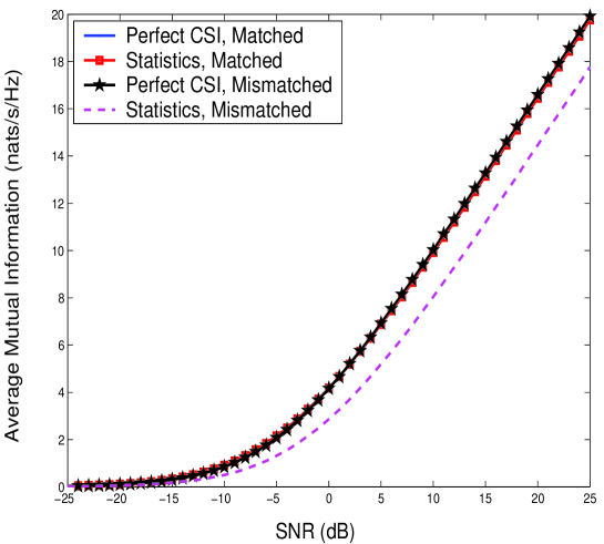
Figure 1: Mutual information of the perfect CSI and the statistical semiunitary precoders over matched and mismatched channels.

• Matched vs. Mismatched Channels: The first study illustrates the performance of statistical semiunitary precoding over matched and mismatched channels. We consider a $4\times 4$ matched channel with normalized separable model, where ${\mathrm{diag}}({\bf\Lambda}_{t})=[8\hskip 3.61371pt8\hskip 3.61371pt0\hskip 3.61371pt0]$. The mismatched channel is characterized by ${\mathrm{diag}}({\bf\Lambda}_{t})=[4\hskip 3.61371pt4\hskip 3.61371pt4\hskip 3.61371pt4]$. In both the cases, ${\bf\Lambda}_{r}=4\hskip 1.4457pt{\bf I}_{4}$. Fig. 1 shows the average mutual information with perfect CSI and statistical semiunitary precoding in the two channels.

  As explained before, the mutual information in the four cases are given by:

  $$I_{{\sf matched},\hskip 1.4457pt{\sf perf}}(\rho)=I_{{\sf matched},\hskip 1.4457pt{\sf stat}}(\rho) = {\mathit{E}}\left[\sum_{i=1}^{M}\log\left(1+\frac{\rho}{M}\hskip 1.4457pt\frac{N_{t}}{M}\hskip 1.4457pt\lambda_{i}(\widetilde{\bf H}_{{\sf{iid}}}^{H}{\widetilde{\bf H}}_{{\sf{iid}}})\right)\right]$$ (56)

  $$I_{{\sf mismatched},\hskip 1.4457pt{\sf perf}}(\rho) = {\mathit{E}}\left[\sum_{i=1}^{M}\log\left(1+\frac{\rho}{M}\hskip 1.4457pt\lambda_{i}({\bf H}_{{\sf{iid}}}^{H}{\bf H}_{{\sf{iid}}})\right)\right]$$ (57)

  $$I_{{\sf mismatched},\hskip 1.4457pt{\sf stat}}(\rho) = {\mathit{E}}\left[\sum_{i=1}^{M}\log\left(1+\frac{\rho}{M}\hskip 1.4457pt\lambda_{i}(\widetilde{\bf H}_{{\sf{iid}}}^{H}{\widetilde{\bf H}}_{{\sf{iid}}})\right)\right],$$ (58)

  where $\widetilde{{\bf H}}_{{\sf{iid}}}$ and ${\bf H}_{{\sf{iid}}}$ are $N_{r}\times M$ and $N_{r}\times N_{t}$ i.i.d. matrices. As can be seen from (56), (58) and Fig. 1, the performance of the mismatched statistical precoder is $10\log_{10}\left(\frac{N_{t}}{M}\right)\approx 3$ dB away from both the matched precoders. It is also surprising that the matched precoders have nearly the same performance as the mismatched (i.i.d. channel) optimal precoder. This seems to be related to the choice of $N_{t},N_{r}$, $M$ and eigen-properties of i.i.d. random matrices.

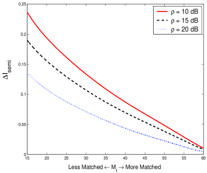
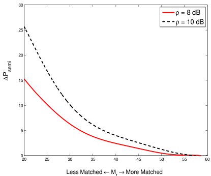
  (a)	(b)

  Figure 2: Gap in performance between statistical and perfect CSI semiunitary precoding as a function of the matching metric, ${\cal M}_{t}$: (a) Mutual information and (b) Error probability.

• Performance Gap as a Function of Matching Metric: The second study focuses on the gap in performance between the perfect CSI and the statistical precoders, as a function of the degree of matching of the channel to the precoder structure. We consider $4\times 4$ channels with $M=2$, and freeze ${\bf U}_{t}$, ${\bf U}_{r}$ to some arbitrary choice in our study. We also freeze ${\bf\Lambda}_{r}$ to $4\hskip 1.4457pt{\bf I}_{4}$ so as to focus on the impact of matching on the transmitter side. Note that the matching metric (defined in Sec. V-E), ${\cal M}_{t}=\prod_{k=1}^{M}{\bf\Lambda}_{t}(k)$, takes values in the range $(0,64]$ in our setting. A family of $\sim{}1700$ channels (each characterized uniquely by ${\bf\Lambda}_{t}(k),{\hskip 3.61371pt}k=1,\cdots,N_{t}$) is generated such that $\sum_{k=1}^{N_{t}}{\bf\Lambda}_{t}(k)=\rho_{c}=16$ and ${\cal M}_{t}$ takes values over its range. The channels become more matched (on the transmitter side) to the precoder structure as ${\cal M}_{t}$ increases.

  While much of our study in the preceding sections is based on asymptotic random matrix theory, Fig. 2 illustrates that the notion of matched channels developed in this work is useful in characterizing performance, even in practically relevant regimes like $4\times 4$ channels. Fig 2(a) illustrates that $\Delta I_{{\sf semi}}$ decreases as the channel becomes more matched on the transmitter side for three choices of $\rho$, whereas Fig 2(b) illustrates the same trend for $\Delta P_{{\sf semi}}$. Note that for a given channel as $\rho$ increases, $\Delta I_{{\sf semi}}$ decreases whereas $\Delta P_{{\sf semi}}$ increases. This is because of the contrasting behaviors of $I_{{\sf{stat}},\hskip 1.4457pt{\sf semi}}(\rho)$ and $P_{{\sf{err}},\hskip 1.4457pt{\sf{perf}},\hskip 1.4457pt{\sf unconst}}(\rho)$ as $\rho$ increases.

  It is important to note the following. In general, there exists no ordering relationship between any two matrix channels [49]. Nevertheless, Fig. 2 shows that the relative (mutual information or error probability) performance of two channels can be compared by using ${\cal M}_{t}$ and ${\cal M}_{r}$. A channel that is more matched leads to a smaller value of $\Delta I_{\bullet}$, as well as $\Delta P_{\bullet}$ for any fixed ${\sf{SNR}}$.

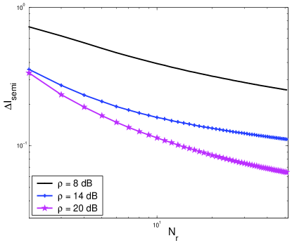
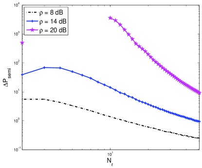
  (a)	(b)

  Figure 3: Asymptotic optimality of the statistical semiunitary precoder for fixed $N_{t}=4$, $M=2$ as $N_{r}$ increases: (a) Mutual information and (b) Error probability.

• Asymptotic Optimality: The third study illustrates the asymptotic optimality of statistical precoding. Fig 3 plots $\Delta I_{{\sf semi}}$ and $\Delta P_{{\sf semi}}$ as a function of $N_{r}$ with $N_{t}$ and $M$ fixed at $N_{t}=4$ and $M=2$. The channels have separable correlation with ${\bf\Lambda}_{t}={\bf I}_{4}$ whereas ${\bf\Lambda}_{r}=\frac{4}{N_{r}}\hskip 1.4457pt{\bf I}_{N_{r}}$ and hence, $\rho_{c}=4$ for all the channels. As can be seen from the study in the previous sections as well as the figures, channel hardening, where the eigenvectors of ${\bf H}^{H}{\bf H}$ converge to the eigenvectors of ${\bf\Sigma}_{t}={\mathit{E}}[{\bf H}^{H}{\bf H}]$ as $\frac{N_{t}}{N_{r}}\rightarrow 0$ ensures that even channel statistical information is as good as perfect CSI with respect to performance.

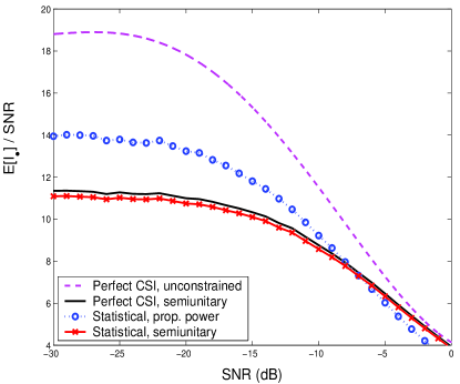
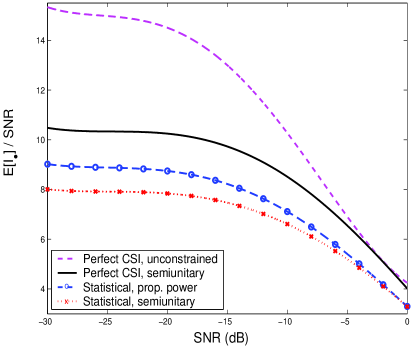
  (a)	(b)

  Figure 4: Low- and medium-${\sf{SNR}}$ mutual information performance of the statistical precoder in (24) when compared with the semiunitary precoder for a) separable and b) non-separable (canonical) models.

• Low- and Medium-${\sf{SNR}}$ Regimes: The last study of this section studies the mutual information performance of a statistical precoder in (24) when compared with a semiunitary precoder in the low- and the medium-${\sf{SNR}}$ regimes. In the high-${\sf{SNR}}$ regime, the optimal perfect CSI precoder excites the $M$ modes uniformly with equal power. However, in the low-${\sf{SNR}}$ regime, the perfect CSI precoder allocates power to the transmit eigen-modes non-uniformly. The precoder structure in (24) excites the $M=2$ modes with power proportional to the transmit eigenvalues and hence, performs better than the semiunitary precoder. Fig 4(a) shows the performance of the statistical precoder in a channel with separable correlation, while Fig. 4(b) corresponds to a channel with non-separable correlation. In the separable case, the transmit and the receive eigenvalues are given by ${\mathrm{diag}}({\bf\Lambda}_{t})=[9.80\hskip 3.61371pt5.66\hskip 3.61371pt0.45\hskip 3.61371pt0.09]$ and ${\mathrm{diag}}({\bf\Lambda}_{r})=[8.58\hskip 3.61371pt4.20\hskip 3.61371pt1.98\hskip 3.61371pt1.24]$ whereas in the canonical case the variance matrix, ${\bf M}=(\sigma_{ij}^{2})$, is given by

  $${\bf M}=\left[\begin{array}[]{cccc}1.66&0.31&1.71&0.31\\ 2.24&0.18&0.15&0.54\\ 1.97&1.46&0.70&0.28\\ 1.65&1.65&0.49&0.71\end{array}\right].$$ (63)

  It is interesting to note that the perfect CSI semiunitary precoder may either perform better or worse than that of the precoder in (24). Future work will look at this aspect more carefully.

IX Concluding Remarks

The main focus of this work is on precoding for spatially correlated multi-antenna channels that are often encountered in practice. Motivated and inspired by many recent wireless standardization efforts, we proposed low-complexity structured precoding techniques in this paper. Here, the eigen-modes of the precoder are chosen to be the dominant eigenvectors of the transmit covariance matrix, whereas the power allocation across the excited modes are obtained via certain simple, low-complexity methods. A special case of structured precoder is a semiunitary precoder, where the spatial modes are excited with uniform power.

In this work, we first established the structure of the optimal perfect CSI structured precoder and showed that it naturally extends the channel diagonalizing architecture of the perfect CSI unconstrained precoder. We motivated the need for a relative difference metric that captures the impact of lack of perfect CSI on the precoder performance, independent of the operating ${\sf{SNR}}$. We then analytically characterized the average relative mutual information loss (as well as the average relative uncoded error probability enhancement) of the statistical semiunitary precoder using tools from random matrix and eigenvector perturbation theories.

Our results show that given a precoder architecture (that is, fixed antenna dimensions and precoder rank), the relative difference metrics are minimized by a channel that is matched to it. A matched channel is one that has: 1) The same number of dominant transmit eigen-modes as the precoder rank, and 2) The dominant transmit as well as the receive eigen-modes that are well-conditioned. Our theoretical study also characterizes matching metrics that enable the comparison of two channels with respect to performance loss captured by the relative difference metrics. In particular, as the channel becomes more matched to the precoder structure and the matching metrics change accordingly continuously, the performance loss decreases monotonically and vice versa. Numerical studies are provided to illustrate our results.

Our work is a first attempt to analytically study the performance of low-complexity statistical precoding with respect to a perfect CSI benchmark. Much of this study has been rendered possible due to substantial advances in capturing the eigen-properties of random matrices with independent entries. Nevertheless, there exist many directions along which this work can be developed. We now list a few of these directions.

This work is limited to the high-${\sf{SNR}}$, large antenna asymptotic regime where a comprehensive random matrix theory is available to capture precoder performance [50]. Even in this regime, it may be possible as in [47] to refine the constants in the bounds for the relative loss terms and obtain further insights on the impact of spatial correlation on performance loss. Besides that, in the case of proportional growth of antenna dimensions with a non-separable correlation model, both mutual information as well as error probability have not been characterized completely in this work. Lack of availability of closed-form mutual information expressions for non-Gaussian inputs limits the development of this work. The notion of precoder-channel matching introduced in this work can be developed further to aid in the design of low-complexity, structured and adaptive signaling schemes. In the case of mismatched channels, the construction of limited feedback schemes to bridge the gap in performance has been undertaken in [13, 51, 52]. The question of trade-offs between spatial versus spatio-temporal precoding [53] and extensions to more general Ricean fading [54], multi-user [55], wideband [56] systems are also of interest.

-A Key Mathematical Results

We now introduce some key mathematical results that will be needed in the ensuing proofs.

Majorization Theory: We start with a few results from majorization theory [49].

Definition 1

Let ${\mathbf{a}}$ and ${\mathbf{b}}$ be two vectors in ${\mathbb{R}}^{m}$ in non-increasing order, i.e., ${\mathbf{a}}(1)\geq\cdots\geq{\mathbf{a}}(m)$ and ${\mathbf{b}}(1)\geq\cdots\geq{\mathbf{b}}(m)$. Then ${\mathbf{a}}$ is majorized by ${\mathbf{b}}$ (denoted by ${\mathbf{a}}\prec{\mathbf{b}}$) if

$$\sum_{i=1}^{k}{\mathbf{a}}(i)\leq\sum_{i=1}^{k}{\mathbf{b}}(i),\hskip 3.61371pt1\leq k\leq m$$ (64)

with equality if $k=m$.

Remark 1

For example, if $m=3$, any positive vector ${\mathbf{a}}$ such that $\sum_{i=1}^{3}{\mathbf{a}}(i)=1$ satisfies the following majorization relationship:

$${\mathbf{a}}_{\sf low}\prec{\mathbf{a}}\prec{\mathbf{a}}_{\sf high}$$ (65)

where ${\mathbf{a}}_{\sf low}=\left[\frac{1}{3}\hskip 7.22743pt\frac{1}{3}\hskip 7.22743pt\frac{1}{3}\right]$ and ${\mathbf{a}}_{\sf high}=\left[1\hskip 7.22743pt0\hskip 7.22743pt0\right]$. Another example of a majorization relationship is provided by an $m\times m$ Hermitian matrix ${\mathbf{X}}$, with $m$-dimensional vectors ${\bf e}$ and ${\bf d}$ denoting the eigenvalues and diagonal entries of ${\mathbf{X}}$, respectively. We have ${\bf d}\prec{\bf e}$. From the definition, it can also be easily checked that if ${\mathbf{a}}\prec{\mathbf{b}}$, then $-{\mathbf{a}}\prec-{\mathbf{b}}$.

Lemma 5

A matrix ${\mathbf{Q}}$ is said to be unitary-stochastic if there exists a unitary matrix ${\mathbf{\Gamma}}$ such that ${\mathbf{Q}}(i,j)=|{\mathbf{\Gamma}}(i,j)|^{2}$ [49, Sec. 2B.5, p. 23]. By definition, a unitary-stochastic matrix is doubly stochastic. If ${\mathbf{u}}\prec{\mathbf{v}}$, there exists a unitary-stochastic matrix ${\mathbf{Q}}$ such that ${\mathbf{u}}={\mathbf{v}}{\mathbf{Q}}$.

Definition 2

Let ${\mathbf{a}}$ and ${\mathbf{b}}$ be two vectors in ${\mathbb{R}}^{m}$ in non-increasing order. Then ${\mathbf{a}}$ is weakly submajorized by ${\mathbf{b}}$ (denoted by ${\mathbf{a}}\prec_{w}{\mathbf{b}}$) if

$$\sum_{i=1}^{k}{\mathbf{a}}(i)\leq\sum_{i=1}^{k}{\mathbf{b}}(i),\hskip 3.61371pt1\leq k\leq m.$$ (66)

If the inequality is in the opposite direction in (66), then ${\mathbf{a}}$ is weakly supermajorized by ${\mathbf{b}}$ and is denoted by ${\mathbf{a}}\prec^{w}{\mathbf{b}}$. Note that if ${\mathbf{a}}\prec_{w}{\mathbf{b}}$, then ${\mathbf{b}}\prec^{w}{\mathbf{a}}$ and vice versa.

Lemma 6

A vector ${\mathbf{a}}$ is submajorized by ${\mathbf{b}}$ if and only if $\sum g({\mathbf{a}}(i))\leq\sum g({\mathbf{b}}(i))$ for all continuous, increasing convex functions $g:{\mathbb{R}}\mapsto{\mathbb{R}}$. For supermajorization, replace $g(\cdot)$ by all continuous, decreasing convex functions. If $g(\cdot)$ is decreasing, convex and ${\mathbf{a}}\prec^{w}{\mathbf{b}}$, we have

$$\left[g({\mathbf{a}}(1))\hskip 3.61371pt\cdots\hskip 3.61371ptg({\mathbf{a}}(m))\right]\hskip 3.61371pt\prec_{w}\hskip 3.61371pt\left[g({\mathbf{b}}(1))\hskip 3.61371pt\cdots\hskip 3.61371ptg({\mathbf{b}}(m))\right].$$ (67)

Proof:

See [49, p. 10] for the first statement. For the second, see [49, p. 116]. ∎

Definition 3

A function $f:{\cal A}\mapsto{\mathbb{R}}$ with ${\cal A}\subset{\mathbb{R}}^{m}$ is said to be Schur-concave on ${\cal A}$ if $\{{\mathbf{a}},{\mathbf{b}}\}\in{\cal A}$ and ${\mathbf{a}}\prec{\mathbf{b}}$ implies that $f({\mathbf{a}})\geq f({\mathbf{b}})$. If however, $f({\mathbf{a}})\leq f({\mathbf{b}})$ for all such ${\mathbf{a}}$ and ${\mathbf{b}}$, $f(\cdot)$ is said to be Schur-convex on ${\cal A}$. If a function is Schur-concave (or -convex) over ${\mathbb{R}}^{m}$, we just say that it is Schur-concave (or -convex). Note that $f(\cdot)$ is Schur-concave if and only if $-f(\cdot)$ is Schur-convex.

Remark 2

An example of Schur-convex and Schur-concave functions is as follows. Let ${\bf x}=\left[x_{1}\hskip 1.4457pt\cdots\hskip 1.4457ptx_{m}\right]$ with $x_{i}\geq x_{i+1}$. Consider the weighted arithmetic mean of $\{x_{i}\}$ given by $f({\bf x})=\sum_{i=1}^{m}w_{i}x_{i}$. The function $f(\cdot)$ is Schur-convex if $w_{i}\geq 0$ and $w_{1}\hskip 1.4457pt\leq\hskip 1.4457pt\cdots\hskip 1.4457pt\leq\hskip 1.4457ptw_{m}$. If $w_{i}\geq 0$, but are in the reverse order, then $f(\cdot)$ is Schur-concave. See [9, Lemma 4] for proof of this claim. It is important to note that the sets of Schur-concave and Schur-convex functions neither partition nor cover the space of all functions, nor are they disjoint.

Lemma 7

Let $f:{\mathbb{R}}\mapsto{\mathbb{R}}$ be a continuous convex function. Then, $\sum_{i=1}^{m}f(x_{i})$ is Schur-convex. That is, if ${\mathbf{u}}$ and ${\mathbf{v}}$ are two $m\times 1$ vectors such that ${\mathbf{u}}\prec{\mathbf{v}}$, then, $\sum_{i=1}^{m}f({\mathbf{u}}(i))\leq\sum_{i=1}^{m}f({\mathbf{v}}(i))$. Let $\phi:{\mathbb{R}}^{m}\mapsto{\mathbb{R}}$ be Schur-convex and the univariate function $\phi(\cdots,x_{i},\cdots):{\mathbb{R}}\mapsto{\mathbb{R}}$ be monotonically decreasing for all $i$. If ${\mathbf{a}}\prec^{w}{\mathbf{b}}$, we have $\phi({\mathbf{a}})\leq\phi({\mathbf{b}})$.

Proof:

See [49, p. 11] for the first statement and [49, p. 59] for the second. ∎

Lemma 8

Let $f:{\mathbb{R}}\mapsto{\mathbb{R}}$ be a continuous convex function. Then, $\max_{i=1,\hskip 3.61371pt\cdots,\hskip 3.61371ptm}f(x_{i})$ is continuous and Schur-convex.

Proof:

A composition of an increasing, Schur-convex function with a convex function results in a Schur-convex function [49, p. 63]. The proof follows by noting that $\max_{i}x_{i}$ is a function that is increasing in its arguments and is Schur-convex. ∎

Lemma 9

Let $\{x_{i},i=1,\cdots,K\}$ and $\{y_{i},i=1,\cdots,K\}$ be two $K$-tuples such that $\{x_{i},y_{i}\}\geq 0$ for all $i$. Then,

$$\sum_{i=1}^{K}x_{i}\leq\frac{1}{K}\left(\sum_{i=1}^{K}\frac{x_{i}}{y_{i}}\right)\left(\sum_{i=1}^{K}y_{i}\right).$$ (68)

Proof:

We prove the lemma by induction. Consider the case $K=2$. Without loss of generality, let $x_{1}\leq x_{2}$ and $y_{1}\geq y_{2}$. We therefore have $\frac{x_{1}}{y_{1}}\leq\frac{x_{2}}{y_{2}}$ which implies that

$$x_{1}+x_{2}\leq\frac{x_{1}}{y_{1}}\hskip 3.61371pty_{2}+\frac{x_{2}}{y_{2}}\hskip 3.61371pty_{1}.$$ (69)

Adding $x_{1}+x_{2}$ on both sides and rearranging, we see that the statement is true for $K=2$. Let the statement be true for $K=n-1$ for any ordering where $x_{1}\leq\cdots\leq x_{n-1}$ and $y_{1}\geq\cdots\geq y_{n-1}$. We will show that the statement is true for the $K=n$ case, where we augment the $(n-1)$-tuples with $x_{n}$ and $y_{n}$. Without loss of generality, we can assume that $x_{1}\leq\cdots\leq x_{n}$ and $y_{1}\geq\cdots\geq y_{n}$ after possible rearrangement and relabeling of indices. We have

$$\sum_{i=1}^{n-1}x_{i}+x_{n} \stackrel{{\scriptstyle(a)}}{{\leq}} \frac{1}{n-1}\left(\sum_{i=1}^{n-1}\frac{x_{i}}{y_{i}}\right)\left(\sum_{i=1}^{n-1}y_{i}\right)+\frac{x_{n}}{y_{n}}\hskip 3.61371pty_{n}$$ (71)

$$\stackrel{{\scriptstyle(b)}}{{=}} \frac{1}{n}\left(\sum_{i=1}^{n-1}\frac{x_{i}}{y_{i}}\right)\left(\sum_{i=1}^{n-1}y_{i}\right)+\frac{1}{n}\frac{x_{n}}{y_{n}}\hskip 3.61371pty_{n}$$

$${\hskip 7.22743pt}+\underbrace{\frac{1}{n(n-1)}\left(\sum_{i=1}^{n-1}\frac{x_{i}}{y_{i}}\right)\left(\sum_{i=1}^{n-1}y_{i}\right)+\frac{n-1}{n}\cdot\frac{x_{n}}{y_{n}}\hskip 3.61371pty_{n}}_{A}$$

$$nA = \left(\sum_{i=1}^{n-1}\frac{x_{i}}{y_{i}}-\frac{(n-1)x_{n}}{y_{n}}\right)\cdot\left(\frac{\sum_{i=1}^{n-1}y_{i}}{n-1}-y_{n}\right)+y_{n}\left(\sum_{i=1}^{n-1}\frac{x_{i}}{y_{i}}\right)+\frac{x_{n}}{y_{n}}\left(\sum_{i=1}^{n-1}y_{i}\right),$$

where (a) follows from the induction hypothesis and (b) by breaking the sum into two pieces. The statement holds for $K=n$ upon rearrangement after using the increasing and decreasing ordering assumption of $x_{i}$ and $y_{i}$, respectively. ∎

Matrix Theory: The Poincare separation theorem connects the eigenvalues of semiunitary transformations with those of the transformed matrix [57, Cor. 4.3.16, p. 190].

Lemma 10

Let ${\mathbf{A}}$ be an $n\times n$ Hermitian matrix. Let $r$ be such that $1\leq r\leq n$ and let ${\mathbf{w}}_{1},\cdots,{\mathbf{w}}_{r}$ be a set of orthonormal vectors in ${\mathbb{C}}^{n}$. Define ${\mathbf{B}}={\mathbf{W}}^{\sl H}{\mathbf{A}}{\mathbf{W}}$ where ${\mathbf{W}}=\left[{\mathbf{w}}_{1}\hskip 3.61371pt\cdots\hskip 3.61371pt{\mathbf{w}}_{r}\right]$. Let the eigenvalues of ${\mathbf{A}}$ and ${\mathbf{B}}$ be arranged in non-increasing order. Then, we have $\lambda_{k}({\mathbf{B}})\leq\lambda_{k}({\mathbf{A}})$ for all $k=1,\cdots,r$.

The following lemma provides bounds for eigenvalues of sums and products of Hermitian matrices [57].

Lemma 11

If ${\bf A}$ and ${\bf B}$ are $n\times n$ Hermitian matrices, then

$$\lambda_{k}({\bf A})\lambda_{\min}({\bf B}) \leq\lambda_{k}({\bf AB})\leq \lambda_{k}({\bf A})\lambda_{\max}({\bf B}),\hskip 7.22743ptk=1,\hskip 3.61371pt\cdots,\hskip 3.61371ptn,$$ (72)

$$\lambda_{k}({\bf A})+\lambda_{\min}({\bf B}) \leq\lambda_{k}({\bf A}+{\bf B})\leq \lambda_{k}({\bf A})+\lambda_{\max}({\bf B}),\hskip 7.22743ptk=1,\hskip 3.61371pt\cdots,\hskip 3.61371ptn.$$ (73)

We also have

$$\sum_{k=1}^{n}\lambda_{k}({\bf AB})\leq\sum_{k=1}^{n}\lambda_{k}({\bf A})\ \lambda_{k}({\bf B}).$$ (74)

The following lemma [58] helps in computing the determinant of partitioned matrices.

Lemma 12

If ${\bf X},{\bf Y},{\bf Z}$ and ${\bf W}$ are $n\times n$ matrices and ${\bf W}$ is invertible, we have

$$\det\left[\begin{array}[]{cc}{\bf X}&{\bf Y}\\ {\bf Z}&{\bf W}\end{array}\right]=\det({\bf X}-{\bf Y}{\bf W}^{-1}{\bf Z})\cdot\det({\bf W}).$$ (77)

Random Matrix Theory: We now characterize the eigenvalues of certain families of random matrices.

Lemma 13

Let ${\bf X}$ be a $p\times n$ complex random matrix with i.i.d. entries of mean zero, common variance $1$ and a finite fourth moment. Consider two cases: 1) $p$ is finite and $n\rightarrow\infty$, and 2) $\{p,n\}\rightarrow\infty$ with $p/n\rightarrow 0$. In either case, in the asymptotics of $n$, the empirical eigenvalue distribution of $\frac{{\bf X}{\bf X}^{\sl H}-n{{\mathbf{I}}}_{p}}{2\sqrt{np}}$ converges pointwise with probability $1$ to the semi-circular law $F(x)$ where,

$$F(x)=\left\{\begin{array}[]{cc}0&{\rm if}\hskip 3.61371ptx<-1,\\ \int_{y=-1}^{x}\frac{2}{\pi}\sqrt{1-y^{2}}\hskip 1.4457pt{\mathrm{d}}y&{\rm if}\hskip 3.61371pt-1\leq x\leq 1,\\ 1&{\rm if}\hskip 3.61371ptx>1.\end{array}\right.$$ (81)

In particular, with probability one, we have

$$1-2\sqrt{\frac{p}{n}}\leq\liminf_{n}\frac{\lambda_{\min}({\bf X}{\bf X}^{\sl H})}{n}\leq\limsup_{n}\frac{\lambda_{\max}({\bf X}{\bf X}^{\sl H})}{n}\leq 1+2\sqrt{\frac{p}{n}}.$$ (82)

Let ${\mathbf{\Lambda}}$ be an $n\times n$ positive definite diagonal matrix. Under the same assumptions on ${\bf X},p,n$ as above, there exists a finite constant $\gamma_{1}>0$ (dependent on $p$ and $n$ only through ${\bf\Lambda}$) such that, with probability $1$

$$\frac{\sum_{i}{\mathbf{\Lambda}}(i)}{n}-\gamma_{1}\sqrt{\frac{p}{n}}\leq\liminf_{n}\frac{\lambda_{\min}({\bf X}{\mathbf{\Lambda}}{\bf X}^{\sl H})}{n}\leq\limsup_{n}\frac{\lambda_{\max}({\bf X}{\mathbf{\Lambda}}{\bf X}^{\sl H})}{n}\leq\frac{\sum_{i}{\mathbf{\Lambda}}(i)}{n}+\gamma_{1}\sqrt{\frac{p}{n}}.$$

On the other hand, let ${\bf X}$ be a $p\times n$ complex random matrix with independent entries from a fixed probability space such that ${\bf X}(i,j)$ is zero mean, has variance $\sigma_{ij}^{2}$ and

$$\sup_{n,p}\max_{ij}{\mathit{E}}[|{\bf X}(i,j)|^{4}]\leq\gamma_{2}<\infty.$$ (83)

Also, without loss of generality, assume that $\big{\{}\sum_{j=1}^{n}\sigma_{ij}^{2}\big{\}}$ are arranged in decreasing order. Then there exists a finite constant $\gamma_{3}>0$ (independent of $p,n$) such that, for all $i$

$$\frac{\sum_{j=1}^{n}\sigma_{ij}^{2}}{n}-\gamma_{3}\sqrt{\frac{p}{n}}\leq\liminf_{n}\frac{\lambda_{i}({\bf X}{\bf X}^{\sl H})}{n}\leq\limsup_{n}\frac{\lambda_{i}({\bf X}{\bf X}^{\sl H})}{n}\leq\frac{\sum_{j=1}^{n}\sigma_{ij}^{2}}{n}+\gamma_{3}\sqrt{\frac{p}{n}}$$ (84)

with probability $1$.

Proof:

We provide an elementary proof of the claim when $p$ is finite, $n\rightarrow\infty$ and ${\bf X}(i,j)$ are standard, complex Gaussian. Define the set $A_{n}\triangleq\Big{\{}\omega:\frac{\lambda_{\max}({\bf X}(\omega){\bf\Lambda}{\bf X}(\omega)^{H})}{n}>1+\epsilon_{1}+\epsilon_{2}\Big{\}}$. If we can show that $\sum_{n}{\rm Pr}\left(A_{n}\right)<\infty$, it follows from the Borel-Cantelli lemma [59] that ${\rm Pr}\left(\limsup A_{n}\right)=0$. By choosing $\epsilon_{1}$ and $\epsilon_{2}$ appropriately (as a function of $n$), we can establish strict bounds on the eigenvalues.

Breaking ${\bf X}{\bf\Lambda}{\bf X}^{H}$ into a diagonal component and an off-diagonal component and using Lemma 11, it follows via a union bound that

$${\rm Pr}\left(A_{n}\right)\leq p{\rm Pr}\left(\frac{\sum_{i=1}^{n}\left(|{\bf X}(1,i)|^{2}-1\right){\bf\Lambda}(i)}{n}>\epsilon_{1}\right)+p^{2}{\rm Pr}\left(\frac{|\sum_{i=1}^{n}{\bf X}(1,i){\bf\Lambda}(i){\bf X}(2,i)^{\star}|}{n}>\epsilon_{2}\right).$$

Using a Chernoff-type bound [59], we have the following:

$${\rm Pr}(A_{n})\leq p\exp\left(-\frac{\epsilon_{1}^{2}n^{2}}{2\sum_{i=1}^{n}({\bf\Lambda}(i))^{2}}\right)+2p^{2}\exp\left(-\frac{\epsilon_{2}^{2}n^{2}c}{\sum_{i=1}^{n}({\bf\Lambda}(i))^{2}}\right)$$ (85)

for some $c>0$. The smallest value of $\epsilon_{1}$ and $\epsilon_{2}$ that can still result in ${\rm Pr}\left(\limsup A_{n}\right)=0$ is such that

$$\epsilon_{1}={\mathcal{O}}(\epsilon_{2})=\sqrt{\frac{\sum_{i=1}^{n}({\bf\Lambda}(i))^{2}}{n}}\cdot\frac{1}{n^{1/2-\eta}},{\hskip 7.22743pt}\eta>0.$$ (86)

Letting $\eta\downarrow 0$, we have

$$\limsup\frac{\lambda_{\max}({\bf X}{\bf\Lambda}{\bf X}^{H})}{n}\leq\frac{\sum_{i=1}^{n}{\bf\Lambda}(i)}{n}+\gamma_{4}\sqrt{\frac{\sum_{i=1}^{n}{\bf\Lambda}(i)^{2}}{n}}\cdot\frac{1}{\sqrt{n}},$$ (87)

where $\gamma_{4}>0$ is a constant independent of $p$ and $n$. The expression for $\lambda_{\min}(\cdot)$ is symmetric with that of $\lambda_{\max}(\cdot)$ and can be obtained similarly. The extension to the case where ${\bf X}$ has only independent entries (not necessarily complex Gaussian) also proceeds via the same logic.

Since $p\rightarrow\infty$ in Case 2), the above technique is not useful in establishing the claim of the lemma. Here, the result follows from [60], [61, Theorem 2.9, p. 623]. The generalizations with ${\bf\Lambda}$ and independent entries follow via the same proof technique as in [60] and hence no proofs are provided. The readers are referred to [61] for a brief summary of the general technique. ∎

-B Proofs of Prop. 1-4

Proof of Prop. 1: Let ${\bf F}$ be a fixed $N_{t}\times M$ semiunitary precoder and define

$${\bf B}\triangleq\left({\mathbf{I}}_{M}+\frac{\rho}{M}{\bf F}^{H}{\bf H}^{H}{\bf H}{\bf F}\right)^{-1}.$$ (88)

From (8), note that the vector ${\sf{MSE}}$ is the vector of diagonal entries of ${\bf B}$. Following Lemma 10, we have $\lambda_{k}\left({\bf F}^{H}{\bf H}^{H}{\bf H}{\bf F}\right)\leq\lambda_{k}\left({\bf H}^{H}{\bf H}\right)$ for $k=1,\cdots,M$. That is, the eigenvalues of ${\bf B}$ satisfy

$$\lambda_{k}({\bf B})\geq\frac{1}{1+\frac{\rho}{M}\lambda_{M-k+1}({\bf H}^{H}{\bf H})},\hskip 3.61371ptk=1,\cdots,M.$$ (89)

Denote by ${\bf\lambda}_{{\bf B}}$ the vector of eigenvalues of ${\bf B}$. The Schur-concavity of $f(\cdot)$ and the fact that the diagonal entries of a Hermitian matrix are majorized by its eigenvalues when used with ${\bf B}$ results in $f\left({\sf{MSE}}\right)\geq f\left({\bf\lambda}_{{\bf B}}\right)$. The monotonicity of $f(\cdot)$ when combined with (89) implies that

$$f\left({\sf{MSE}}\right)\geq f\left(\left[\cdots,\hskip 3.61371pt\frac{1}{1+\frac{\rho}{M}\lambda_{M-k+1}({\bf H}^{H}{\bf H})},\hskip 3.61371pt\cdots\right]\right).$$ (90)

Note that the lower bound in (90) is independent of the choice of ${\bf F}$, and hence, also serves as a universal lower bound. Furthermore, the choice of ${\bf F}$ in (9) meets the lower bound and is hence optimal.

Proof of Prop. 2: Let ${\bf F}$ be a fixed semiunitary matrix. Define the $M\times 1$ vectors ${\bf d}$ and ${\bf e}$ with ${\bf d}(k)\triangleq{\mathbf{B}}(k)$, where ${\mathbf{B}}=\left({\mathbf{I}}_{M}+\frac{\rho}{M}{\bf F}^{H}{\bf H}^{H}{\bf H}{\bf F}\right)^{-1}$ and ${\bf e}(k)\triangleq\frac{1}{M}\sum_{i=1}^{M}\frac{1}{1+\frac{\rho}{M}\lambda_{i}\left({\bf F}^{H}{\bf H}^{H}{\bf H}{\bf F}\right)}$, respectively. Note that ${\bf e}(k)$ is equal for all $k$ and hence, from Remark 1 we have ${\bf d}\succ{\bf e}$. From Lemma 7, we have that $\sum_{k=1}^{M}h(\cdot)$ is Schur-convex. Hence,

$$\sum_{k=1}^{M}h\left({\bf d}(k)\right) \geq \sum_{k=1}^{M}h\left({\bf e}(k)\right)=Mh\left({\bf e}(1)\right).$$ (91)

Using Lemma 10 and the increasing property of $h(\cdot)$, we have

$$\sum_{k=1}^{M}h\left({\bf d}(k)\right) \geq Mh\left(\frac{1}{M}\sum_{k=1}^{M}\frac{1}{1+\frac{\rho}{M}\lambda_{k}({\mathbf{H}}^{H}{\mathbf{H}})}\right).$$ (92)

Since the right-hand side of (92) is independent of the choice of ${\bf F}$, it serves as a lower bound on the error probability.

Our goal is to show that the lower bound can be achieved and the choice of ${\bf F}$ that leads to the lower bound is ${\bf F}_{{\sf{opt}}}$. For this, let $A$ be defined as $A\triangleq\frac{1}{M}\sum_{i=1}^{M}\frac{1}{1+\frac{\rho}{M}\lambda_{i}({\mathbf{H}}^{H}{\mathbf{H}})}$. Further, define the two $M\times 1$ vectors ${\mathbf{u}}$ and ${\mathbf{v}}$ such that ${\mathbf{u}}(k)=A$ for all $k$ and ${\mathbf{v}}(k)=\frac{1}{1+\frac{\rho}{M}\lambda_{k}({\mathbf{H}}^{H}{\mathbf{H}})}$. Since ${\mathbf{u}}\prec{\mathbf{v}}$, from Lemma 5, there exists a unitary-stochastic matrix ${\mathbf{Q}}$ such that ${\mathbf{u}}={\mathbf{v}}{\mathbf{Q}}$ with ${\mathbf{Q}}(i,j)=|{\mathbf{\Gamma}}(i,j)|^{2}$ for some ${\mathbf{\Gamma}}$ unitary. Consider the precoder ${\bf F}$ as given in (12). The ${\sf{MSE}}$ across the data-streams with this precoder is given by

$${\sf{MSE}}_{k} = \left[{\bf B}^{-1}\right]_{k}=\left[\left({\mathbf{I}}_{M}+\frac{\rho}{M}{\bf F}^{H}\hskip 1.4457pt{\bf H}^{H}\hskip 1.4457pt{\bf H}\hskip 1.4457pt{\bf F}\right)^{-1}\right]_{k}$$ (93)

$$= \left[\left({\mathbf{I}}_{M}+\frac{\rho}{M}{\mathbf{\Gamma}}^{H}\hskip 1.4457pt\widehat{\bf\Lambda}\hskip 1.4457pt{\mathbf{\Gamma}}\right)^{-1}\right]_{k}=\left[{\mathbf{\Gamma}}^{H}\hskip 1.4457pt\left({\mathbf{I}}_{M}+\frac{\rho}{M}\widehat{\bf\Lambda}\right)^{-1}\hskip 1.4457pt{\mathbf{\Gamma}}\right]_{k}$$ (94)

with $\widehat{{\bf\Lambda}}(k)=\lambda_{k}({\bf H}^{H}{\bf H})$. From the definitions of ${\mathbf{\Gamma}}$, ${\bf v}$ and the relationship ${\bf u}={\bf v}{\mathbf{Q}}$, it is easy to check that ${\sf{MSE}}_{k}=A$ for all $k$. Thus, with the choice of ${\bf F}$ as in (12), we can achieve the lower bound in (92).

Proof of Prop. 4: For the Schur-concave case, from Lemma 10 and (74), it can be checked that ${\bf a}\prec_{w}{\bf b}$, where ${\bf a}(k)=\lambda_{k}({\bf\Lambda}_{{\sf fixed}}\hskip 1.4457pt{\bf V}_{\bf F}^{H}\hskip 1.4457pt{\bf H}^{H}\hskip 1.4457pt{\bf H}\hskip 1.4457pt{\bf V}_{\bf F})$ and ${\bf b}(k)={\bf\Lambda}_{{\sf fixed}}(k)\hskip 3.61371pt\lambda_{k}({\bf H}^{H}{\bf H})$. Define $g(y)=\frac{1}{1+\kappa y}$ for some fixed $\kappa>0$ and note that $g(\cdot)$ is convex and decreasing. Thus, from Lemma 6 we have $g({\mathbf{b}})\prec_{w}g({\mathbf{a}})$. Noting that $-f(\cdot)$ is Schur-convex and decreasing, from Lemma 7 we have $f\left(g({\mathbf{a}})\right)\geq f\left(g({\mathbf{b}})\right)$. This universal lower bound is achievable by ${\bf F}_{{\sf{opt}}}$ as in (17).

When $f(\cdot)$ is Schur-convex, we proceed similar to the semiunitary case. Using $g(y)=\frac{1}{1+\kappa y}$, from Lemma 6, we have

$$\sum_{k=1}^{M}g({\bf b}(k))\leq\sum_{k=1}^{M}g({\bf a}(k)).$$ (95)

Define ${\bf u}(k)=\frac{1}{M}\sum_{i=1}^{M}\frac{1}{1+\frac{\rho}{M}{\bf\Lambda}_{{\sf fixed}}(i)\hskip 1.4457pt\lambda_{i}({\bf H}^{H}{\bf H})}$ for all $k$ and ${\bf w}(k)=\frac{1}{1+\frac{\rho}{M}{\bf\Lambda}_{{\sf fixed}}(k)\hskip 1.4457pt\lambda_{k}({\bf H}^{H}{\bf H})}$, and note that ${\bf u}\prec{\bf w}$. That is, there exists a unitary-stochastic ${\bf Q}$ such that ${\bf u}={\bf v}{\bf Q}$. The result follows as before.

-C Proof of Proposition 5

To characterize the behavior of $\Delta I_{1}$, recall the structure of the optimal semiunitary precoder from Prop. 1 and note from Lemma 2 that the perfect CSI unconstrained scheme corresponds to waterfilling along the first $M$ dominant transmit singular vectors. Thus, we have

$$\Delta I_{1}\cdot{\mathit{E}}_{{\mathbf{H}}}\left[I_{{\sf{stat}},\hskip 3.61371pt{\sf semi}}(\rho)\right] = {\mathit{E}}_{{\mathbf{H}}}\left[\sum_{i=1}^{n_{{\mathbf{H}}}}\log\left(1+{\bf\Lambda}_{{\mathbf{H}}}(i){\bf\Lambda}_{\sf wf}(i)\right)-\sum_{i=1}^{M}\log\left(1+\frac{\rho}{M}\hskip 3.61371pt{\bf\Lambda}_{{\mathbf{H}}}(i)\right)\right],$$ (96)

where for each realization ${\mathbf{H}}$, $n_{{\mathbf{H}}}$ modes are excited ($1\leq n_{{\mathbf{H}}}\leq M$) with power ${\bf\Lambda}_{\sf wf}(i)\triangleq\left(\mu_{{\mathbf{H}}}-\frac{1}{{\bf\Lambda}_{{\mathbf{H}}}(i)}\right)^{+}$ and the water level $\mu_{{\mathbf{H}}}$ is chosen such that $\sum_{i=1}^{n_{{\mathbf{H}}}}{\bf\Lambda}_{\sf wf}(i)=\rho$. It can be easily checked that ${\bf\Lambda}_{\sf wf}(i)$ can be written as

$${\bf\Lambda}_{\sf wf}(i)=\frac{\rho}{n_{{\mathbf{H}}}}+\frac{1}{n_{{\mathbf{H}}}}\sum_{j=1}^{n_{{\mathbf{H}}}}\frac{1}{{\bf\Lambda}_{{\mathbf{H}}}(j)}-\frac{1}{{\bf\Lambda}_{{\mathbf{H}}}(i)},$$ (97)

and $n_{{\mathbf{H}}}$ is the largest value of $k$ that satisfies:

$$\sum_{i=1}^{k}\frac{{\bf\Lambda}_{{\mathbf{H}}}(i)-{\bf\Lambda}_{{\mathbf{H}}}(k)}{{\bf\Lambda}_{{\mathbf{H}}}(i){\bf\Lambda}_{{\mathbf{H}}}(k)}\leq\rho.$$ (98)

Hence, we have

$$\Delta I_{1}\cdot{\mathit{E}}_{{\mathbf{H}}}\left[I_{{\sf{stat}},\hskip 3.61371pt{\sf semi}}(\rho)\right] \leq {\mathit{E}}_{{\mathbf{H}}}\left[\sum_{i=1}^{n_{{\mathbf{H}}}}\log\left(1+\frac{\frac{\rho{\bf\Lambda}_{{\mathbf{H}}}(i)(M-n_{{\mathbf{H}}})}{n_{{\mathbf{H}}}M}-1+\frac{{\bf\Lambda}_{{\mathbf{H}}}(i)}{n_{{\mathbf{H}}}}\sum_{j=1}^{n_{{\mathbf{H}}}}\frac{1}{{\bf\Lambda}_{{\mathbf{H}}}(j)}}{1+\frac{\rho{\bf\Lambda}_{{\mathbf{H}}}(i)}{M}}\right)\right].$$ (99)

Using the fact that $\log(1+x)\leq x$ for all $x>-1$, after some simplifications we can further upper bound $\Delta I_{1}$ as

$$\Delta I_{1}\cdot{\mathit{E}}_{{\mathbf{H}}}\left[I_{{\sf{stat}},\hskip 3.61371pt{\sf semi}}(\rho)\right] \leq {\mathit{E}}_{{\mathbf{H}}}\left[M-n_{{\mathbf{H}}}\right]+\frac{M^{2}}{\rho^{2}}\cdot{\mathit{E}}_{{\mathbf{H}}}\left[\sum_{i=1}^{M}\frac{1}{{\bf\Lambda}_{{\mathbf{H}}}(i)^{2}}\right].$$ (100)

From (98), it is easily recognized that if $\rho\geq\frac{k}{{\bf\Lambda}_{{\mathbf{H}}}(k)}-\sum_{i=1}^{k}\frac{1}{{\bf\Lambda}_{{\mathbf{H}}}(i)}$, and in particular, if $\rho\geq\frac{k}{{\bf\Lambda}_{{\mathbf{H}}}(k)}$, then $n_{{\mathbf{H}}}\geq k$. Thus, if $\rho>\alpha{\mathit{E}}_{{\mathbf{H}}}\left[\frac{M}{{\bf\Lambda}_{{\mathbf{H}}}(M)}\right]$ for some $\alpha>1$ as in the statement of the theorem, both the terms in (100) can be bounded by constants that depend only on the channel statistics. For this note that,

$${\mathit{E}}_{{\mathbf{H}}}\left[M-n_{{\mathbf{H}}}\right] \leq M\cdot{\rm Pr}(n_{{\mathbf{H}}}<M)\leq M\cdot{\rm Pr}\left(\frac{M}{{\bf\Lambda}_{{\mathbf{H}}}(M)}>\rho\right)$$ (101)

$$\leq M\cdot{\rm Pr}\left(\frac{1}{{\bf\Lambda}_{{\mathbf{H}}}(M)}>\alpha{\mathit{E}}\left[\frac{1}{{\bf\Lambda}_{{\mathbf{H}}}(M)}\right]\right)\stackrel{{\scriptstyle(a)}}{{\leq}}\frac{M}{\alpha^{2}}\cdot\frac{{\mathit{E}}\left[\left(\frac{1}{{\bf\Lambda}_{{\mathbf{H}}}(M)}\right)^{2}\right]}{\left({\mathit{E}}\left[\frac{1}{{\bf\Lambda}_{{\mathbf{H}}}(M)}\right]\right)^{2}},$$ (102)

where (a) follows from Chebyshev’s inequality. A trivial upper bound for the other term gives the desired result.

-D Proof of Theorem 1

It can be checked that $\widetilde{\Delta I}_{2}$ can be written as

$$\widetilde{\Delta I}_{2} = {\mathit{E}}_{{\bf H}}\Bigg{[}\frac{\sum_{k=1}^{M}\log\big{(}1+\frac{\rho}{M}\hskip 1.4457pt\lambda_{k}({\bf H}^{\sl H}{\bf H})\big{)}}{\sum_{k=1}^{M}\log\big{(}1+\frac{\rho}{M}\hskip 1.4457pt\lambda_{k}({\bf F}_{{\sf semi}}^{H}{\bf H}^{\sl H}{\bf H}{\bf F}_{{\sf semi}})\big{)}}-1\Bigg{]}$$ (103)

$$\stackrel{{\scriptstyle(a)}}{{\leq}} {\mathit{E}}_{{\bf H}}\left[\frac{1}{M}\sum_{k=1}^{M}\frac{\log\big{(}1+\frac{\rho}{M}\hskip 1.4457pt\lambda_{k}({\bf H}^{\sl H}{\bf H})\big{)}}{\log\big{(}1+\frac{\rho}{M}\hskip 1.4457pt\lambda_{k}({\bf F}_{{\sf semi}}^{H}{\bf H}^{\sl H}{\bf H}{\bf F}_{{\sf semi}})\big{)}}-1\right]$$ (104)

$$\stackrel{{\scriptstyle(b)}}{{=}} \frac{1}{M}\sum_{k=1}^{M}{\mathit{E}}_{{\bf H}}\left[\frac{\log\Big{(}1+\frac{\rho}{M\hskip 1.4457pt\rho_{c}}\hskip 1.4457pt\lambda_{k}({\mathbf{\Lambda}}_{t}\hskip 1.4457pt{\bf H}_{{\sf{iid}}}^{\sl H}\hskip 1.4457pt{\mathbf{\Lambda}}_{r}\hskip 1.4457pt{\bf H}_{{\sf{iid}}})\Big{)}}{\log\Big{(}1+\frac{\rho}{M\hskip 1.4457pt\rho_{c}}\hskip 1.4457pt\lambda_{k}({\widetilde{{\mathbf{\Lambda}}}}_{t}\hskip 1.4457pt{\bf\widetilde{H}}_{{\sf{iid}}}^{\sl H}\hskip 1.4457pt{\mathbf{\Lambda}}_{r}\hskip 1.4457pt{\bf\widetilde{H}}_{{\sf{iid}}})\Big{)}}-1\right],$$ (105)

where (a) follows from Lemma 9, and (b) from the notations established in Sec. IV-A.

Using Lemmas 11 and 13, we have the following in the limit of $N_{r},\hskip 1.4457ptN_{t},\hskip 1.4457ptM$:

$$\widetilde{\Delta I}_{2} \leq \frac{1}{M}\sum_{k=1}^{M}{\mathit{E}}_{{\mathbf{H}}}\left[\frac{\log\left(1+\frac{\rho}{M\hskip 1.4457pt\rho_{c}}{\bf\Lambda}_{t}(k)\lambda_{\max}({\mathbf{H}}_{{\sf{iid}}}^{H}{\bf\Lambda}_{r}{\mathbf{H}}_{{\sf{iid}}})\right)}{\log\left(1+\frac{\rho}{M\hskip 1.4457pt\rho_{c}}{\bf\Lambda}_{t}(k)\lambda_{\min}(\widetilde{{\mathbf{H}}}_{{\sf{iid}}}^{H}{\bf\Lambda}_{r}\widetilde{{\mathbf{H}}}_{{\sf{iid}}})\right)}-1\right]$$ (106)

$$\leq \frac{1}{M}\sum_{k=1}^{M}{\mathit{E}}_{{\mathbf{H}}}\left[\frac{\log\left(1+\frac{\rho}{M}{\bf\Lambda}_{t}(k)\hskip 1.4457pt\left(1+\kappa_{1}\frac{\sqrt{\sum_{i}({\bf\Lambda}_{r}(i))^{2}}}{\rho_{c}}\right)\right)}{\log\left(1+\frac{\rho}{M}{\bf\Lambda}_{t}(k)\hskip 1.4457pt\left(1-\kappa_{1}\frac{\sqrt{\sum_{i}({\bf\Lambda}_{r}(i))^{2}}}{\rho_{c}}\right)\right)}-1\right]$$ (107)

$$\leq \frac{2\kappa_{1}\sqrt{\sum_{i}({\bf\Lambda}_{r}(i))^{2}}}{\rho_{c}}\cdot\frac{1}{M}\sum_{k=1}^{M}\left[\frac{1}{\log\left(1+\frac{\rho}{M}{\bf\Lambda}_{t}(k)\right)}\right],$$ (108)

where $\kappa_{1}$ is the constant from an application of Lemma 13 in this setting. The last inequality follows by using the log-inequality and some trivial manipulations. The proof is complete.

-E Proof of Proposition 6

We have the following well-known facts [42]:

$$I_{{\sf{perf}}}(\rho)=\log\big{(}1+\rho\hskip 1.4457pt\lambda_{\max}({\bf H}^{H}{\bf H})\big{)}, I_{{\sf{stat}}}(\rho)=\log\bigg{(}1+\rho\sum_{k=1}^{N_{t}}\lambda_{k}|{\mathbf{v}}_{k}^{\sl H}{\mathbf{u}}_{{\sf{stat}}}|^{2}\bigg{)},$$ (109)

where ${\bf u}_{{\sf{stat}}}$ is an eigenvector corresponding to the dominant eigenvalue of ${\bf\Sigma}_{t}={\mathit{E}}[{\mathbf{H}}^{H}{\mathbf{H}}]$, and an eigen-decomposition of ${\mathbf{H}}^{H}{\mathbf{H}}$ is of the form: ${\mathbf{H}}^{H}{\mathbf{H}}=\sum_{k=1}^{N_{t}}\lambda_{k}{\bf v}_{k}{\bf v}_{k}^{H}$. The following simplifications can then be made:

$${{\mathit{E}}}_{{\mathbf{H}}}\left[I_{{\sf{stat}}}(\rho)\right]\cdot\Delta I_{\sf bf} = {\mathit{E}}_{{\mathbf{H}}}\bigg{[}\log\bigg{(}1+\rho\hskip 3.61371pt\frac{\lambda_{1}-\sum_{k}\lambda_{k}|{\mathbf{v}}_{k}^{\sl H}{\mathbf{u}}_{{\sf{stat}}}|^{2}}{1+\rho\sum_{k}\lambda_{k}|{\mathbf{v}}_{k}^{\sl H}{\mathbf{u}}_{{\sf{stat}}}|^{2}}\bigg{)}\bigg{]}$$ (110)

$$\stackrel{{\scriptstyle(a)}}{{\leq}} {\mathit{E}}_{{\mathbf{H}}}\left[\log\left(1+\rho\hskip 1.4457pt\lambda_{1}\hskip 1.4457pt(1-|{\mathbf{v}}_{1}^{\sl H}{\mathbf{u}}_{{\sf{stat}}}|^{2})\right)\right]$$ (111)

$$\stackrel{{\scriptstyle(b)}}{{\leq}} \log\left(1+\rho{\mathit{E}}_{{\mathbf{H}}}\left[\lambda_{\max}({\bf H}^{H}{\bf H})(1-|{\mathbf{v}}_{1}^{\sl H}{\mathbf{u}}_{{\sf{stat}}}|^{2})\right]\right)$$ (112)

$$\stackrel{{\scriptstyle(c)}}{{\leq}} \log\left(1+\rho\cdot\sqrt{{\mathit{E}}_{{\mathbf{H}}}\left[(1-|{\mathbf{v}}_{1}^{\sl H}{\mathbf{u}}_{{\sf{stat}}}|^{2})^{2}\right]}\cdot\sqrt{{\mathit{E}}_{{\mathbf{H}}}\left[\lambda_{\max}^{2}({\bf H}^{H}{\bf H})\right]}\right),$$ (113)

where (a) follows trivially by ignoring the contribution of $k=2,\hskip 1.4457pt\cdots,\hskip 1.4457ptN_{t}$ in the summation, (b) follows from Jensen’s inequality, and (c) from Cauchy-Schwarz inequality. We use the eigenvector perturbation theory developed in [14] and in particular, the bound in [14, Eqn. (16)] to establish that

$${\mathit{E}}_{{\mathbf{H}}}\left[(1-|{\mathbf{v}}_{1}^{\sl H}{\mathbf{u}}_{{\sf{stat}}}|^{2})^{2}\right]\leq\kappa_{3}^{\prime}\hskip 1.4457pt\frac{N_{t}\log(N_{r})}{N_{r}}$$ (114)

for some appropriate constant $\kappa_{3}^{\prime}$ that is independent of the channel statistics and dimensions. Using Lemma 11 and Lemma 13, the conclusion in (36) follows for the relative asymptotics case. For the proportional growth case, an upper bound needs to be established for ${\mathit{E}}_{{\mathbf{H}}}\left[\lambda_{\max}^{2}({\bf H}^{H}{\bf H})\right]$. See [62] for an upper bound technique that builds on the work by [63], which results in the statement of the theorem.

-F Proof of Theorem 3

As in App. -D, we can write $\Delta I_{2}$ as

$$\Delta I_{2} = \frac{{\mathit{E}}_{{\bf H}}[I_{{\sf{perf}},\hskip 1.4457pt{\sf semi}}(\rho)]}{{\mathit{E}}_{{\bf H}}[I_{{\sf{stat}},\hskip 1.4457pt{\sf semi}}(\rho)]}-1$$ (115)

$$= \frac{{\mathit{E}}_{{\bf H}}\left[\sum_{k=1}^{M}\log\big{(}1+\frac{\rho}{M}\hskip 1.4457pt\lambda_{k}({\bf H}^{\sl H}{\bf H})\big{)}\right]}{{\mathit{E}}_{{\bf H}}\left[\sum_{k=1}^{M}\log\big{(}1+\frac{\rho}{M\hskip 1.4457pt\rho_{c}}\lambda_{k}(\widetilde{{\mathbf{\Lambda}}}_{t}\widetilde{{\mathbf{H}}}_{{\sf{iid}}}^{H}{\mathbf{\Lambda}}_{r}\widetilde{{\mathbf{H}}}_{{\sf{iid}}})\big{)}\right]}-1.$$ (116)

The denominator of (116) can be computed following the method in [50, Theorem 1] and equals

$${\mathit{E}}_{{\mathbf{H}}}[I_{{\sf{stat}},\hskip 1.4457pt{\sf semi}}(\rho)]=\sum_{k=1}^{M}\log\left(1+\frac{\rho}{\rho_{c}}\hskip 1.4457pt\mu_{1}{\mathbf{\Lambda}}_{t}(k)\right)+\sum_{k=1}^{M}\log\left(1+\frac{\rho}{\rho_{c}}\hskip 1.4457pt\widetilde{\mu}_{1}{\mathbf{\Lambda}}_{r}(k)\right)-\frac{\rho M}{\rho_{c}}\hskip 1.4457pt\mu_{1}\widetilde{\mu}_{1},$$ (117)

where $\mu_{1}$ and $\widetilde{\mu}_{1}$ satisfy the recursive equations

$$\mu_{1}=\frac{1}{M}\sum_{k=1}^{M}\frac{{\mathbf{\Lambda}}_{r}(k)}{1+\frac{\rho}{\rho_{c}}\hskip 1.4457pt\widetilde{\mu}_{1}{\mathbf{\Lambda}}_{r}(k)}, \widetilde{\mu}_{1}=\frac{1}{M}\sum_{k=1}^{M}\frac{{\mathbf{\Lambda}}_{t}(k)}{1+\frac{\rho}{\rho_{c}}\hskip 1.4457pt{\mu}_{1}{\mathbf{\Lambda}}_{t}(k)}.$$ (118)

A simple lower bound for ${\mathit{E}}_{{\mathbf{H}}}[I_{{\sf{stat}},\hskip 1.4457pt{\sf semi}}(\rho)]$ is obtained by using $\log(1+x)\geq\log(x)$ for $x>0$:

$${\mathit{E}}_{{\mathbf{H}}}[I_{{\sf{stat}},\hskip 1.4457pt{\sf semi}}(\rho)]\geq\sum_{k=1}^{M}\log\left(\frac{\rho^{2}}{\rho_{c}^{2}e}\mu_{1}\widetilde{\mu}_{1}{\bf\Lambda}_{t}(k){\bf\Lambda}_{r}(k)\right).$$ (119)

We now establish that the above bound is order-optimal as $\alpha$ increases (with $\rho=\alpha\frac{M}{{\bf\Lambda}_{t}(M)}$), by lower bounding $\mu_{1}\widetilde{\mu}_{1}$. We can easily show that

$$\mu_{1}\geq\frac{\rho_{c}}{M}\cdot\frac{b_{2}}{1+\alpha b_{1}\frac{{\bf\Lambda}_{r}(1)}{{\bf\Lambda}_{t}(M)}},{\hskip 14.45377pt}\widetilde{\mu}_{1}\geq\frac{\rho_{c}}{M}\cdot\frac{b_{1}}{1+\alpha b_{2}\frac{{\bf\Lambda}_{t}(1)}{{\bf\Lambda}_{t}(M)}},$$ (120)

and hence,

$$1\geq\frac{\rho}{\rho_{c}}\mu_{1}\widetilde{\mu}_{1}\geq\frac{\alpha C_{1}}{1+\alpha(C_{1}+C_{2})},$$ (121)

where $C_{1}=b_{1}\frac{{\bf\Lambda}_{r}(M)}{{\bf\Lambda}_{t}(M)}$ and $C_{2}=b_{2}\frac{{\bf\Lambda}_{t}(1)}{{\bf\Lambda}_{t}(M)}$. Tightness of the bound in (119) follows from using the fact that $\log(1+x)\leq\log(x)+\frac{1}{x},\hskip 1.4457ptx>0$.

Combining the above relationships, we have

$${\mathit{E}}_{{\mathbf{H}}}[I_{{\sf{stat}},\hskip 1.4457pt{\sf semi}}(\rho)] \geq M\log\left(\frac{\rho\alpha C_{1}}{e\left(1+\alpha(C_{1}+C_{2})\right)}\right)+\sum_{k=1}^{M}\log\left(\frac{{\mathbf{\Lambda}}_{t}(k){\mathbf{\Lambda}}_{r}(k)}{\rho_{c}}\right).$$ (122)

Proceeding in the same way, one can obtain an upper bound for ${\mathit{E}}_{{\mathbf{H}}}[I_{{\sf{perf}},\hskip 1.4457pt{\sf semi}}(\rho)]$. Since the main goal here is to obtain the trends of $\Delta I_{2}$, we find it convenient and less cumbersome to replace the upper bound with an approximation ($\log(1+x)\approx\log(x)$) by ignoring the term that decays as $\frac{1}{x}$. Thus, we have

$${\mathit{E}}_{{\mathbf{H}}}[I_{{\sf{perf}},\hskip 1.4457pt{\sf semi}}(\rho)] \approx M\log\left(\frac{\rho}{M}\right)+{\mathit{E}}_{{\mathbf{H}}}\left[\sum_{k=1}^{M}\log\left(\frac{\lambda_{k}({\mathbf{\Lambda}}_{t}{\mathbf{H}}_{{\sf{iid}}}^{H}{\mathbf{\Lambda}}_{r}{\mathbf{H}}_{{\sf{iid}}})}{\rho_{c}}\right)\right]$$ (123)

$$\stackrel{{\scriptstyle(a)}}{{\leq}} M\log\left(\frac{\rho}{M}\right)+\min(A,B)$$ (124)

$$A = M{\mathit{E}}_{{\mathbf{H}}}\left[\log\left(\frac{\lambda_{\max}({\mathbf{H}}_{{\sf{iid}}}^{H}{\mathbf{\Lambda}}_{r}{\mathbf{H}}_{{\sf{iid}}})}{\rho_{c}}\right)\right]+\sum_{k=1}^{M}\log\left({\mathbf{\Lambda}}_{t}(k)\right)$$ (125)

$$B = M{\mathit{E}}_{{\mathbf{H}}}\left[\log\left(\frac{\lambda_{\max}({\mathbf{H}}_{{\sf{iid}}}{\mathbf{\Lambda}}_{t}{\mathbf{H}}_{{\sf{iid}}}^{H})}{\rho_{c}}\right)\right]+\sum_{k=1}^{M}\log\left({\mathbf{\Lambda}}_{r}(k)\right),$$ (126)

where in (a) we have used Lemma 10. Combining (122) and (124), we have the statement of the theorem.

-G Proof of Proposition 7

First, we write $\Delta P_{\sf semi}$ in terms of ${\sf{SINR}}$ of the individual data-streams by using $P_{k,\bullet}=\alpha{\cal Q}\left(\beta({\sf{SINR}}_{k,\bullet})^{1/2}\right)$ and the expression for ${\sf{SINR}}_{k,\bullet}$ in (8). Then, we use the following bound for ${\cal Q}(x)$:

$$\frac{\exp(-x^{2}/2)}{x\sqrt{2\pi}}\left(1-\frac{1}{x^{2}}\right)\leq{\cal Q}(x)\leq\frac{\exp(-x^{2}/2)}{x\sqrt{2\pi}}$$ (127)

to establish the expression in (44). It is straightforward to check that

$${\sf{SINR}}_{k,\hskip 1.4457pt{\sf{perf}},\hskip 1.4457pt{\sf unconst}}={\bf\Lambda}_{\sf wf}(k)\hskip 1.4457pt\lambda_{k}({\bf H}^{H}{\bf H}),$$ (128)

where the waterfilling power allocation $\{{\bf\Lambda}_{\sf wf}(k)\}$ is as in (97) (see App. -C) and normalized to

$$\sum_{k=1}^{M}{\bf\Lambda}_{\sf wf}(k)=\rho.$$ (129)

Similarly, we have

$${\sf{SINR}}_{k,\hskip 1.4457pt{\sf{stat}},\hskip 1.4457pt{\sf semi}}=\frac{1}{\left[{\bf G}^{-1}\right]_{k}}-1 = \frac{\det({\bf G})}{\left[{\rm adj}({\bf G})\right]_{k}}-1,$$ (130)

$${\bf G}={{\mathbf{I}}}_{M}+\frac{\rho}{M}\hskip 1.4457pt{\bf F}_{{\sf semi}}^{H}{\bf H}^{\sl H}{\bf H}{\bf F}_{{\sf semi}} = {{\mathbf{I}}}_{M}+\frac{\rho}{M\hskip 1.4457pt\rho_{c}}\cdot{\widetilde{{\mathbf{\Lambda}}}}_{t}^{1/2}\hskip 1.4457pt{\bf\widetilde{H}}_{{\sf{iid}}}^{\sl H}\hskip 1.4457pt{\mathbf{\Lambda}}_{r}\hskip 1.4457pt{\bf\widetilde{H}}_{{\sf{iid}}}\hskip 1.4457pt{\widetilde{{\mathbf{\Lambda}}}}_{t}^{1/2}.$$ (131)

The matrix ${\rm adj}({\bf G})$ refers to the adjoint of ${\bf G}$, and $\left[{\bf G}^{-1}\right]_{k}$ and $\left[{\rm adj}({\bf G})\right]_{k}$ refer to the $k$-th diagonal entries of ${\bf G}^{-1}$ and ${\rm adj}({\bf G})$, respectively. Using the definition of adjoint of a matrix, we have

$$\left[{\rm adj}({\bf G})\right]_{k} = \det\left({{\mathbf{I}}}_{M-1}+\frac{\rho}{M\hskip 1.4457pt\rho_{c}}\cdot{\widehat{{\mathbf{\Lambda}}}}_{t}^{1/2}\hskip 1.4457pt{\bf\widehat{H}}_{{\sf{iid}}}^{\sl H}\hskip 1.4457pt{\mathbf{\Lambda}}_{r}\hskip 1.4457pt{\bf\widehat{H}}_{{\sf{iid}}}\hskip 1.4457pt{\widehat{{\mathbf{\Lambda}}}}_{t}^{1/2}\right),$$ (132)

where ${\widehat{{\mathbf{\Lambda}}}}_{t}$ and ${\bf\widehat{H}}_{{\sf{iid}}}$ are as per the notations established in Sec. IV-A. The expression for $\Delta{\sf{SINR}}_{k}$ in the statement of the proposition follows immediately.

-H Proof of Theorem 4

We have the following upper bound for ${\sf{SINR}}_{k,\hskip 1.4457pt{\sf{perf}},\hskip 1.4457pt{\sf unconst}}$:

$${\sf{SINR}}_{k,\hskip 1.4457pt{\sf{perf}},\hskip 1.4457pt{\sf unconst}} = {\bf\Lambda}_{\sf wf}(k)\cdot\frac{\lambda_{k}\left({\mathbf{\Lambda}}_{t}\hskip 1.4457pt{{\mathbf{H}}}_{{\sf{iid}}}^{\sl H}\hskip 1.4457pt{\mathbf{\Lambda}}_{r}\hskip 1.4457pt{{\mathbf{H}}}_{{\sf{iid}}}\right)}{\rho_{c}}$$ (133)

$$\stackrel{{\scriptstyle(a)}}{{\leq}} {\bf\Lambda}_{\sf wf}(k)\hskip 1.4457pt{\bf\Lambda}_{t}(k)\cdot\frac{\lambda_{\max}({{\mathbf{H}}}_{{\sf{iid}}}^{\sl H}\hskip 1.4457pt{\mathbf{\Lambda}}_{r}\hskip 1.4457pt{{\mathbf{H}}}_{{\sf{iid}}})}{\rho_{c}},$$ (134)

where (a) follows from Lemma 11. To compute ${\sf{SINR}}_{k,\hskip 1.4457pt{\sf{stat}},\hskip 1.4457pt{\sf semi}}$, note that $\det({\bf G})$, where ${\bf G}$ is as in (131) can be written as

$$\det({\bf G}) = \prod_{j=1}^{M}\left(1+\frac{\rho}{M\hskip 1.4457pt\rho_{c}}\cdot\lambda_{j}({\widetilde{{\mathbf{\Lambda}}}}_{t}\hskip 1.4457pt{\bf\widetilde{H}}_{{\sf{iid}}}^{\sl H}\hskip 1.4457pt{\mathbf{\Lambda}}_{r}\hskip 1.4457pt{\bf\widetilde{H}}_{{\sf{iid}}})\right)$$ (135)

$$\stackrel{{\scriptstyle(a)}}{{\geq}} \prod_{j=1}^{M}\left(1+\frac{\rho}{M\hskip 1.4457pt\rho_{c}}\cdot{\mathbf{\Lambda}}_{t}(j)\hskip 1.4457pt\lambda_{\min}({\bf\widetilde{H}}_{{\sf{iid}}}^{\sl H}\hskip 1.4457pt{\mathbf{\Lambda}}_{r}\hskip 1.4457pt{\bf\widetilde{H}}_{{\sf{iid}}})\right),$$ (136)

with (a) following from Lemma 11. Similarly, we have

$$\left[{\rm adj}({\bf G})\right]_{k} = \prod_{j=1}^{M-1}\left(1+\frac{\rho}{M\hskip 1.4457pt\rho_{c}}\cdot\lambda_{j}({\widehat{{\mathbf{\Lambda}}}}_{t}\hskip 1.4457pt{\bf\widehat{H}}_{{\sf{iid}}}^{\sl H}\hskip 1.4457pt{\mathbf{\Lambda}}_{r}\hskip 1.4457pt{\bf\widehat{H}}_{{\sf{iid}}})\right)$$ (137)

$$\leq \prod_{j=1,\hskip 1.4457ptj\neq k}^{M}\left(1+\frac{\rho}{M\hskip 1.4457pt\rho_{c}}\cdot{\mathbf{\Lambda}}_{t}(j)\hskip 1.4457pt\lambda_{\max}({\bf\widehat{H}}_{{\sf{iid}}}^{\sl H}\hskip 1.4457pt{\mathbf{\Lambda}}_{r}\hskip 1.4457pt{\bf\widehat{H}}_{{\sf{iid}}})\right).$$ (138)

Using Lemma 13 from App. -A in (130) and (134), the following bounds hold with probability $1$ (in the limit of $N_{r},N_{t},M$) for ${\sf{SINR}}_{k,\hskip 1.4457pt{\sf{perf}},\hskip 1.4457pt{\sf unconst}}$ and ${\sf{SINR}}_{k,\hskip 1.4457pt{\sf{stat}},\hskip 1.4457pt{\sf semi}}$:

$${\sf{SINR}}_{k,\hskip 1.4457pt{\sf{perf}},\hskip 1.4457pt{\sf unconst}} \leq {\bf\Lambda}_{\sf wf}(k)\hskip 1.4457pt{\mathbf{\Lambda}}_{t}(k)\cdot\left(1+\frac{C_{1}}{\gamma_{r}}\sqrt{\frac{N_{t}}{N_{r}}}\hskip 1.4457pt\right),$$ (139)

$$1+{\sf{SINR}}_{k,\hskip 1.4457pt{\sf{stat}},\hskip 1.4457pt{\sf semi}} \geq \frac{\prod_{j=1}^{M}\left(1+\frac{\rho}{M}\cdot{\mathbf{\Lambda}}_{t}(j)\hskip 1.4457pt\left(1-\frac{C_{1}}{\gamma_{r}}\sqrt{\frac{M}{N_{r}}}\hskip 1.4457pt\right)\right)}{\prod_{j=1,\hskip 1.4457ptj\neq k}^{M}\left(1+\frac{\rho}{M}\cdot{\mathbf{\Lambda}}_{t}(j)\hskip 1.4457pt\left(1+\frac{C_{1}}{\gamma_{r}}\sqrt{\frac{M-1}{N_{r}}}\hskip 1.4457pt\right)\right)}$$ (140)

for some universal constant $C_{1}$ obtained from Lemma 13. If $\rho$ is such that $\rho\geq\alpha\frac{M}{{\bf\Lambda}_{t}(M)}$, we can trivially lower bound ${\sf{SINR}}_{k,\hskip 1.4457pt{\sf{stat}},\hskip 1.4457pt{\sf semi}}$ as

$$1+{\sf{SINR}}_{k,\hskip 1.4457pt{\sf{stat}},\hskip 1.4457pt{\sf semi}} \geq \left(1+\frac{\rho}{M}\hskip 1.4457pt{\bf\Lambda}_{t}(k)\hskip 1.4457pt\left(1-\frac{C_{1}}{\gamma_{r}}\sqrt{\frac{M}{N_{r}}}\right)\right)\left(\frac{1+\frac{1}{\alpha}-\frac{C_{1}}{\gamma_{r}}\sqrt{\frac{M}{N_{r}}}}{1+\frac{1}{\alpha}+\frac{C_{1}}{\gamma_{r}}\sqrt{\frac{M-1}{N_{r}}}}\right)^{M-1}$$

$$\stackrel{{\scriptstyle(a)}}{{\geq}} \left(1+\frac{\rho}{M}\hskip 1.4457pt{\bf\Lambda}_{t}(k)\hskip 1.4457pt\left(1-\frac{C_{1}}{\gamma_{r}}\sqrt{\frac{M}{N_{r}}}\right)\right)\cdot\left(\frac{1+(M-1)\left(\frac{1}{\alpha}-\frac{C_{1}}{\gamma_{r}}\sqrt{\frac{M}{N_{r}}}\right)}{1+2(M-1)\left(\frac{1}{\alpha}+\frac{C_{1}}{\gamma_{r}}\sqrt{\frac{M-1}{N_{r}}}\right)}\right),$$

(142)

where (a) follows from the fact that $1+ax\leq(1+x)^{a}\leq 1+2ax$ for $x$ sufficiently small and $a>0$. After some routine manipulations, $\Delta{\sf{SINR}}_{k}$ can be bounded as

$$\Delta{\sf{SINR}}_{k} \leq M\left(\frac{1}{\alpha}+\frac{3C_{1}}{\gamma_{r}}\sqrt{\frac{M}{N_{r}}}\right)+{\bf\Lambda}_{t}(k)\left({\bf\Lambda}_{\sf wf}(k)-\frac{\rho}{M}\right)\left(1+\frac{C_{1}}{\gamma_{r}}\sqrt{\frac{N_{t}}{N_{r}}}\right)$$ (143)

$${\hskip 14.45377pt}+\frac{\rho}{M}{\bf\Lambda}_{t}(k)\left(\frac{M}{\alpha}\left(1+\frac{C_{1}}{\gamma_{r}\hskip 1.4457pt\sqrt{N_{r}}}(2\sqrt{N_{t}}+\sqrt{M})\right)+\frac{C_{1}}{\gamma_{r}\hskip 1.4457pt\sqrt{N_{r}}}(3M\sqrt{M}+\sqrt{N_{t}})\right)$$

$$= \frac{M}{\alpha}\left(1+\frac{\rho{\bf\Lambda}_{t}(k)}{M}\right)+{\bf\Lambda}_{t}(k)\cdot\left({\bf\Lambda}_{\sf wf}(k)-\frac{\rho}{M}\right)+\frac{\rho{\bf\Lambda}_{t}(k)}{\gamma_{r}}\cdot{\mathcal{O}}\left(\frac{\sqrt{M}+\sqrt{N_{t}}}{\sqrt{N_{r}}}\right).$$

We now use the facts that $\sqrt{1+x}\leq 1+\frac{x}{2}$ for any $x$ positive, and $\frac{1}{1-x}$ is upper bounded by $1+2x$ as long as $x<\frac{1}{2}$ for the terms $\sqrt{1+\frac{\Delta{\sf{SINR}}_{k}}{{\sf{SINR}}_{k,\hskip 1.4457pt{\sf{stat}},\hskip 1.4457pt{\sf semi}}}}$ and $\frac{1}{1-\frac{1}{\beta^{2}{\sf{SINR}}_{k,\hskip 1.4457pt{\sf{perf}},\hskip 1.4457pt{\sf unconst}}}}$, respectively. The term $\exp\left(\frac{\beta^{2}\Delta{\sf{SINR}}_{k}}{2}\right)$ is bounded by using the fact that $e^{x}$ can be bounded by $1+ax$ for some $a>1$ in the small $x$ regime. The combination of the above facts yields

$$\Delta P_{\sf semi} \leq \frac{1}{M\hskip 1.4457pt\beta^{2}}{\mathit{E}}_{{\mathbf{H}}}\left[\sum_{k=1}^{M}\frac{1}{{\bf\Lambda}_{t}(k){\bf\Lambda}_{\sf wf}(k)}\right]+\beta^{2}\frac{M}{\alpha}+\frac{\beta^{2}}{M}{\mathit{E}}_{{\mathbf{H}}}\left[\sum_{k=1}^{M}{\bf\Lambda}_{t}(k)\left({\bf\Lambda}_{\sf wf}(k)-\frac{\rho}{M}\right)\right]$$ (144)

$${\hskip 14.45377pt}+\frac{\rho\beta^{2}\sum_{k=1}^{M}{\bf\Lambda}_{t}(k)}{M}\left(\frac{1}{\alpha}+\frac{1}{\gamma_{r}}\hskip 3.61371pt{\mathcal{O}}\left(\frac{\sqrt{N_{t}}+\sqrt{M}}{\sqrt{N_{r}}}\right)\right)$$

up to a constant scaling multiplicative constant on the right side. For the first term, we lower bound ${\bf\Lambda}_{\sf wf}(k)$ from (97) by

$${\bf\Lambda}_{\sf wf}(k) \geq \frac{\rho}{n_{{\mathbf{H}}}}-\frac{1}{{\bf\Lambda}_{{\mathbf{H}}}(k)}\stackrel{{\scriptstyle(a)}}{{\geq}}\frac{\rho}{M}-\frac{1}{{\bf\Lambda}_{t}(k)\left(1-\frac{C_{1}}{\gamma_{r}}\sqrt{\frac{N_{t}}{N_{r}}}\right)},$$ (145)

where (a) follows from Lemma 13. For the third term, we have

$${\mathit{E}}_{{\mathbf{H}}}\left[\sum_{k=1}^{M}{\bf\Lambda}_{t}(k)\left({\bf\Lambda}_{\sf wf}(k)-\frac{\rho}{M}\right)\right]\leq M+\rho\sum_{k=1}^{M}{\bf\Lambda}_{t}(k)\cdot\left({\mathit{E}}_{{\mathbf{H}}}\left[\frac{1}{n_{{\mathbf{H}}}}\right]-\frac{1}{M}\right).$$ (146)

Finally, we have

$${\mathit{E}}_{{\mathbf{H}}}\left[\frac{1}{n_{{\mathbf{H}}}}-\frac{1}{M}\right] \leq \left(1-\frac{1}{M}\right){\rm Pr}(n_{{\mathbf{H}}}<M)\leq\frac{1}{\alpha^{2}}\cdot\frac{{\mathit{E}}\left[\left(\frac{1}{{\bf\Lambda}_{{\mathbf{H}}}(M)}\right)^{2}\right]}{\left({\mathit{E}}\left[\frac{1}{{\bf\Lambda}_{{\mathbf{H}}}(M)}\right]\right)^{2}},$$ (147)

where the second inequality follows from the bound in (102). Combining these facts, we have

$$\Delta P_{\sf semi} \leq \frac{1}{\beta^{2}M}\sum_{k=1}^{M}\frac{1}{\frac{\rho{\bf\Lambda}_{t}(k)}{M}-1}+\beta^{2}(1+\frac{M}{\alpha})$$ (148)

$${\hskip 1.4457pt}+\frac{\beta^{2}\rho\sum_{k=1}^{M}{\bf\Lambda}_{t}(k)}{M}\left(\frac{1}{\alpha}+\frac{1}{\alpha^{2}}\cdot\frac{{\mathit{E}}\left[\left(\frac{1}{{\bf\Lambda}_{{\mathbf{H}}}(M)}\right)^{2}\right]}{\left({\mathit{E}}\left[\frac{1}{{\bf\Lambda}_{{\mathbf{H}}}(M)}\right]\right)^{2}}+\frac{1}{\gamma_{r}}\hskip 3.61371pt{\mathcal{O}}\left(\frac{\sqrt{N_{t}}+\sqrt{M}}{\sqrt{N_{r}}}\right)\right)$$

Thus the proof is complete.

References

• [1] K. H. Lee and D. P. Petersen, “Optimal Linear Coding for Vector Channels,” IEEE Trans. Commun., vol. 24, no. 12, pp. 1283–1290, Dec. 1976.
• [2] J. Salz, “Digital Transmission over Cross-Coupled Linear Channels,” AT&T Tech. Journal, vol. 64, no. 6, pp. 1147–1159, July-Aug. 1985.
• [3] J. Yang and S. Roy, “On Joint Transmitter and Receiver Optimization for Multiple-Input-Multiple-Output (MIMO) Transmission Systems,” IEEE Trans. Commun., vol. 42, no. 12, pp. 3221–3231, Dec. 1994.
• [4] A. Scaglione, G. B. Giannakis, and S. Barbarossa, “Redundant Filterbank Precoders and Equalizers Part I: Unification and Optimal Designs,” IEEE Trans. Sig. Proc., vol. 47, no. 7, pp. 1988–2006, July 1999.
• [5] H. Sampath, P. Stoica, and A. Paulraj, “Generalized Linear Precoder and Decoder Design for MIMO Channels Using the Weighted MMSE Criterion,” IEEE Trans. Commun., vol. 49, no. 12, pp. 2198–2206, Dec. 2001.
• [6] H. Sampath and A. Paulraj, “Linear Precoding for Space-Time Coded Systems with Known Fading Correlations,” IEEE Commun. Letters, vol. 6, no. 6, pp. 239–241, June 2002.
• [7] J. Yang and S. Roy, “Joint Transmitter-Receiver Optimization for Multi-input Multi-output Systems with Decision Feedback,” IEEE Trans. Inform. Theory, vol. 40, no. 5, pp. 1334–1347, Sept. 1994.
• [8] A. Scaglione, P. Stoica, S. Barbarossa, G. B. Giannakis, and H. Sampath, “Optimal Designs for Space-Time Linear Precoders and Decoders,” IEEE Trans. Sig. Proc., vol. 50, no. 5, pp. 1051–1064, May 2002.
• [9] D. P. Palomar, J. M. Cioffi, and M. A. Lagunas, “Joint Tx-Rx Beamforming Design for Multicarrier MIMO Channels: A Unified Framework for Convex Optimization,” IEEE Trans. Sig. Proc., vol. 51, no. 9, pp. 2381–2401, Sept. 2003.
• [10] A. J. Goldsmith, S. A. Jafar, N. Jindal, and S. Vishwanath, “Capacity Limits of MIMO Channels,” IEEE Journ. Selected Areas in Commun., vol. 21, no. 5, pp. 684–702, June 2003.
• [11] D. Gesbert, H. Bolcskei, D. A. Gore, and A. J. Paulraj, “Outdoor MIMO Wireless Channels: Models and Performance Prediction,” IEEE Trans. Commun., vol. 50, no. 12, pp. 1926–1934, Dec. 2002.
• [12] D. J. Love and R. W. Heath, Jr., “Limited Feedback Diversity Techniques for Correlated Channels,” IEEE Trans. Veh. Tech., vol. 55, no. 2, pp. 718–722, Mar. 2006.
• [13] V. Raghavan, V. V. Veeravalli, and A. M. Sayeed, “Quantized Multimode Precoding in Spatially Correlated Multi-Antenna Channels,” Submitted to IEEE Trans. Sig. Proc., Dec. 2007, Available: [Online]. http://www.ifp.uiuc.edu/$\sim$vasanth.
• [14] V. Raghavan, R. W. Heath, Jr., and A. M. Sayeed, “Systematic Codebook Designs for Quantized Beamforming in Correlated MIMO Channels,” IEEE Journ. Selected Areas in Commun., vol. 25, no. 7, pp. 1298–1310, Sept. 2007.
• [15] R. W. Keyes, “Physical Limits in Digital Electronics,” Proc. IEEE, vol. 63, no. 5, pp. 740–767, May 1975.
• [16] J. D. Meindl and J. A. Davis, The Fundamental Limit on Binary Switching Energy for Terascale Integration (TSI),” IEEE Journ. Solid State Circuits, vol. 35, no. 10, pp. 1515–1516, Oct. 2000.
• [17] J. Rabaey, A. Chandrakasan, and B. Nikolic, Digitial Integrated Circuits: A Design Perspective, Prentice Hall, 2nd edition, 2003.
• [18] B. Razavi, RF Microelectronics, Prentice Hall, Upper Saddle River, NJ, 1998.
• [19] P. G. Y-Massaad, M. Medard, and L. Zheng, “Impact of Processing Energy on the Capacity of Wireless Channels,” Proc. IEEE Intern. Symp. on Inform. Theory and its Appl. (ISITA), 2004.
• [20] A. M. Sayeed and V. V. Veeravalli, “Essential Degrees of Freedom in Space-Time Fading Channels,” Proc. IEEE Intern. Symp. Personal Indoor and Mobile Radio Commun., vol. 4, pp. 1512–1516, Sept. 2002.
• [21] V. V. Veeravalli, Y. Liang, and A. M. Sayeed, “Correlated MIMO Rayleigh Fading Channels: Capacity, Optimal Signaling and Asymptotics,” IEEE Trans. Inform. Theory, vol. 51, no. 6, pp. 2058–2072, June 2005.
• [22] A. S. Y. Poon, R. W. Brodersen, and D. N. C. Tse, “Degrees of Freedom in Multiple-Antenna Channels: A Signal Space Approach,” IEEE Trans. Inform. Theory, vol. 51, no. 2, pp. 523–536, Feb. 2005.
• [23] E. Visotsky and U. Madhow, “Space-Time Transmit Precoding with Imperfect Feedback,” IEEE Trans. Inform. Theory, vol. 47, no. 6, pp. 2632–2639, Sept. 2001.
• [24] S. A. Jafar and A. J. Goldsmith, “Transmitter Optimization and Optimality of Beamforming for Multiple Antenna Systems with Imperfect Feedback,” IEEE Trans. Wireless Commun., vol. 3, no. 4, pp. 1165–1175, July 2004.
• [25] E. Jorswieck and H. Boche, “Channel Capacity and Capacity-Range of Beamforming in MIMO Wireless Systems under Correlated Fading with Covariance Feedback,” IEEE Trans. Wireless Commun., vol. 52, no. 10, pp. 1654–1657, Oct. 2004.
• [26] A. L. Moustakas, S. H. Simon, and A. M. Sengupta, “MIMO Capacity through Correlated Channels in the Presence of Correlated Interferers and Noise,” IEEE Trans. Inform. Theory, vol. 49, no. 10, pp. 2545–2561, Oct. 2003.
• [27] S. Zhou and G. B. Giannakis, “Optimal Transmitter Eigen-Beamforming and Space-Time Block Coding Based on Channel Mean Feedback,” IEEE Trans. Sig. Proc., vol. 50, no. 10, pp. 1599–1613, Oct. 2002.
• [28] A. M. Tulino, A. Lozano, and S. Verdú, “Impact of Antenna Correlation on the Capacity of Multiantenna Channels,” IEEE Trans. Inform. Theory, vol. 51, no. 7, pp. 2491–2509, July 2005.
• [29] H. Venkatachari and M. Varanasi, “Maximizing Mutual Information in General MIMO Fading Channels under Rank Constraint,” Proc. IEEE Asilomar Conf. Signals, Systems and Computers, Nov. 2007.
• [30] X. Zhang, D. P. Palomar, and B. Ottersten, “Robust Design of Linear MIMO Transceivers,” To appear in IEEE Trans. Sig. Proc., 2008.
• [31] M. Skoglund and G. Jongren, “On the Capacity of a Multiple-Antenna Communication Link with Channel Side Information,” IEEE Journ. Selected Areas in Commun., vol. 21, no. 3, pp. 395–405, Apr. 2003.
• [32] J. Akhtar and D. Gesbert, “Spatial Multiplexing over Correlated MIMO Channels with a Closed Form Precoder,” IEEE Trans. Wireless Commun., vol. 4, no. 5, pp. 2400–2409, Sept. 2005.
• [33] W. Weichselberger, M. Herdin, H. Ozcelik, and E. Bonek, “A Stochastic MIMO Channel Model with Joint Correlation of Both Link Ends,” IEEE Trans. Wireless Commun., vol. 5, no. 1, pp. 90–100, Jan. 2006.
• [34] V. Raghavan, J. H. Kotecha, and A. M. Sayeed, “Canonical Statistical Models for Correlated MIMO Fading Channels and Capacity Analysis,” Submitted to IEEE Trans. Inform. Theory, Nov. 2007, Available: [Online]. http://www.ifp.uiuc.edu/$\sim$vasanth.
• [35] C.-N. Chuah, J. M. Kahn, and D. N. C. Tse, “Capacity Scaling in MIMO Wireless Systems under Correlated Fading,” IEEE Trans. Inform. Theory, vol. 48, no. 3, pp. 637–650, Mar. 2002.
• [36] A. M. Sayeed, “Deconstructing Multi-Antenna Fading Channels,” IEEE Trans. Sig. Proc., vol. 50, no. 10, pp. 2563–2579, Oct. 2002.
• [37] D. J. Love, R. W. Heath, Jr., W. Santipach, and M. L. Honig, “What is the Value of Limited Feedback for MIMO Channels?,” IEEE Commun. Magaz., vol. 42, no. 10, pp. 54–59, Oct. 2004.
• [38] K. Yu, M. Bengtsson, B. Ottersten, D. McNamara, P. Karlsson, and M. Beach, “Second Order Statistics of NLOS indoor MIMO Channels based on 5.2 GHz Measurements,” Proc. IEEE Global Telecommun. Conf., vol. 1, pp. 25–29, Nov. 2001.
• [39] H. Ozcelik, M. Herdin, W. Weichselberger, J. Wallace, and E. Bonek, “Deficiencies of ’Kronecker’ MIMO Radio Channel Model,” Electronics Letters, vol. 39, no. 16, pp. 1209–1210, Aug. 2003.
• [40] J. Wallace, H. Ozcelik, M. Herdin, E. Bonek, and M. Jensen, “Power and Complex Envelope Correlation for Modeling Measured Indoor MIMO Channels: A Beamforming Evaluation,” Proc. IEEE Fall Vehicular Technology Conf., vol. 1, pp. 363–367, Oct. 2003.
• [41] Y. Zhou, M. Herdin, A. M. Sayeed, and E. Bonek, “Experimental Study of MIMO Channel Statistics and Capacity via the Virtual Representation,” Tech. Rep., University of Wisconsin-Madison, May 2006, Available: [Online]. http://dune.ece.wisc.edu.
• [42] A. Paulraj, R. Nabar, and D. Gore, Introduction to Space-Time Wireless Communications, Cambridge Univ. Press, 2003.
• [43] D. J. Love and R. W. Heath, Jr., “Multimode Precoding for MIMO Wireless Systems,” IEEE Trans. Sig. Proc., vol. 53, no. 10, pp. 3674–3687, Oct. 2005.
• [44] J. G. Proakis, Digital Communications, McGraw-Hill, 4th edition, 2000.
• [45] V. Raghavan, V. V. Veeravalli, and R. W. Heath, Jr., “Reduced Rank Signaling in Spatially Correlated MIMO Channels,” Proc. IEEE Intern. Symp. Inform. Theory, 2007.
• [46] D. Guo, S. Shamai, and S. Verdú, “Mutual Information and Minimum Mean-Square Error in Gaussian Channels,” IEEE Trans. Inform. Theory, vol. 51, no. 4, pp. 1261–1282, Apr 2005.
• [47] A. Forenza, M. Mckay, A. Pandharipande, R. W. Heath, Jr., and I. B. Collings, “Adaptive MIMO Transmission for Exploiting the Capacity of Spatially Correlated MIMO Channels,” IEEE Trans. Veh. Tech., vol. 56, no. 2, pp. 619–630, Mar. 2007.
• [48] V. Raghavan, A. M. Sayeed, and N. Boston, “Near-Optimal Codebook Constructions for Limited Feedback Beamforming in Correlated MIMO Channels with Few Antennas,” Proc. IEEE Intern. Symp. Inform. Theory, pp. 2622–2626, July 2006.
• [49] A. W. Marshall and I. Olkin, Inequalities: Theory of Majorization and its Applications, Academic Press, NY, 1979.
• [50] W. Hachem, O. Khorunzhiy, Ph. Loubaton, J. Najim, and L. Pastur, “A New Approach for Capacity Analysis for Large Dimensional Multi-Antenna Channels,” To appear in IEEE Trans. Inform. Theory, 2008.
• [51] J. C. Roh and B. D. Rao, “Multiple Antenna Channels with Partial Channel State Information at the Transmitter,” IEEE Trans. Wireless Commun, vol. 3, no. 2, pp. 677–688, Mar. 2004.
• [52] V. K. N. Lau, Y. Liu, and T. A. Chen, “On the Design of MIMO Block Fading Channels with Feedback Link Capacity Constraint,” IEEE Trans. Commun., vol. 52, no. 1, pp. 62–70, Jan. 2004.
• [53] C. Lin, V. Raghavan, and V. V. Veeravalli, “To Code or Not to Code Across Time: Space-Time Coding with Feedback,” To appear in IEEE Journ. Selected Areas in Commun., 2008.
• [54] G. Taricco, “On the Capacity of Separately-Correlated MIMO Rician Fading Channels,” Proc. IEEE Global Telecommun. Conf., 2006.
• [55] N. Jindal, “MIMO Broadcast Channels with Finite Rate Feedback,” IEEE Trans. Inform. Theory, vol. 52, no. 11, pp. 5045–5059, Nov. 2006.
• [56] N. Khaled, B. Mondal, R. W. Heath, Jr., G. Leus, and F. Petre, “Interpolation Based Multi-Mode Precoding for MIMO-OFDM Systems with Limited Feedback,” IEEE Trans. Wireless Commun., vol. 6, no. 3, pp. 1003–1013, Mar. 2007.
• [57] R. A. Horn and C. R. Johnson, Matrix Analysis, Cambridge University Press, 1985.
• [58] J. R. Silvester, “Determinants of Block Matrices,” The Mathematical Gazette, vol. 84, no. 501, pp. 460–467, Nov. 2000.
• [59] R. A. Durrett, Probability: Theory and Examples, Duxbury Press, 2nd edition, 1995.
• [60] Z. D. Bai and Y. Q. Yin, “Convergence to the Semi-Circle Law,” Annals Prob., vol. 16, no. 2, pp. 863–875, 1988.
• [61] Z. D. Bai, “Methodologies in Spectral Analysis of Large Dimensional Random Matrices, A Review,” Statistica Sinica, vol. 9, pp. 611–677, 1999.
• [62] V. Raghavan and A. M. Sayeed, “Role of Channel Power in the Sub-Linear Capacity Scaling of MIMO Channels,” Proc. Allerton Conf. on Commun., Control, and Computing, 2004, Available: [Online]. http://www.ifp.uiuc.edu/$\sim$vasanth.
• [63] Y. Q. Yin, Z. D. Bai, and P. R. Krishnaiah, “On Limit of the Largest Eigenvalue of the Large Dimensional Sample Covariance Matrix,” Probability Theory and Related Fields, vol. 78, pp. 509–521, 1988.