Andreev Transport through Side-Coupled Double Quantum Dots

Abstract

We study the transport through side-coupled double quantum dots, connected to normal and superconducting (SC) leads with a T-shape configuration. We find, using the numerical renormalization group, that the Coulomb interaction suppresses SC interference in the side dot, and enhances the conductance substantially in the Kondo regime. This behavior stands in total contrast to a wide Kondo valley seen in the normal transport. The SC proximity penetrating into the interfacial dot pushes the Kondo clouds, which screens the local moment in the side dot, towards the normal lead to make the singlet bond long. The conductance shows a peak of unitary limit as the cloud expands. Furthermore, two separate Fano structures appear in the gate-voltage dependence of the Andreev transport, where a single reduced plateau appears in the normal transport.

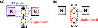
Figure 1: (color online) Quantum dots coupled to (a) a normal lead (N) and superconductor (S), and (b) two normal leads. QD1 (QD2) is referred to as the interfacial (side) dot. Dashed line illustrates a dominant singlet pair in the Kondo cloud.

I Introduction

Observation of the Kondo effect in a quantum dot (QD) Gold_Cronen has stimulated researches in the field of quantum transport, and recent experimental developments enable one to examine the Kondo physics in a variety of systems, such as an Aharonov-Bohm (AB) ring with a QD and double quantum dots (DQD). In these systems multiple paths for electron propagation also affect the tunneling currents, and the interference causes Fano-type asymmetric line shapes.

Superconductivity also brings rich and interesting features into the quantum transport. Competition between superconductivity and the Kondo effect has been reported to be observed in carbon nanotube QD and in semiconductor nanowires. Buit:2002 ; Eich:2007 ; Sand:2007 ; Buiz:2007 ; Grov:2007 ; SDQDS_exp Furthermore, interplay between the Andreev scattering and the Kondo effect has been studied intensively for a QD coupled to a normal (N) lead and superconductor (S), theoretically Fazio ; Schwab ; Clerk ; Sun ; Cuevas ; Avishai1 ; Aono ; Krawiec ; Splett ; Doma ; Avishai2 ; TanakaNQDS and experimentally. Graber So far, however, the Andreev-Kondo physics has been discussed mainly for a single dot. In this paper, we consider a DQD system with a T-shape geometry as shown in Fig. 1, and study how multiple paths affect the interplay at low temperatures, using the numerical renormalization group (NRG) method. Wilkins Golub and Avishai calculated first, to our knowledge, the Andreev transport through an AB ring with a QD,Avishai2 in which a similar interference effect is expected. However, the underlying Kondo physics in such a combination with superconductivity and interference is still not fully understood, and is needed to be clarified precisely, as measurements are being not impossible. SDQDS_exp

We find that the Coulomb interaction in the side dot (QD2 in Fig. 1) suppresses destructive interference typical of the T-shape geometry, and it enhances substantially the tunneling current between the normal and superconducting (SC) leads in the Kondo regime. This is quite different from the behavior seen in the normal transport in the same configuration Fig. 1 (b), for which the conductance is suppressed, and shows a wide minimum called a Kondo valley as a result of strong interference by the Kondo resonance in the side dot. Kim ; Taka ; Corna ; YT:2005 ; Zitko ; Karr ; Rams ; Maruyama2004 The SC proximity penetrating into the interfacial dot (QD1 in Fig. 1) causes this stark contrast between the Andreev and normal transports. It also changes the Fano line shape in the gate-voltage dependence of the conductance. Furthermore, we show that the proximity deforms the Kondo cloud to make a singlet bond long, and it can be deduced from the Fermi-liquid properties of the ground state.

In Sec. II, we introduce the model and describe the effective Hamiltonian in a large gap limit. In Sec. III, we show the numerical results and clarify the transport properties using the renormalized parameters. The Fano structures in the gate-voltage dependence of the conductance are also discussed. A brief summary is given in the last section.

II Model

We start with an Anderson impurity connected to SC and normal leads,

$$\,H=H_{DQD}+H_{S}+H_{N}+H_{T,S}+H_{T,N},$$ (1)

where

$$H_{DQD}=\sum_{i=1,2}\left\{\left(\varepsilon_{d,i}+\frac{U_{i}}{2}\right)\left(n_{i}-1\right)+\frac{U_{i}}{2}\left(n_{i}-1\right)^{2}\right\}$$

$$\qquad\qquad+t\,\sum_{\sigma}\left(d_{1\sigma}^{{\dagger}}d_{2\sigma}+\textrm{H.c.}\right),$$

$$H_{S}=\sum_{k,\sigma}\varepsilon_{k}c_{S,k\sigma}^{\dagger}c_{S,k\sigma}-\sum_{k}\left(\Delta\,c_{S,k\uparrow}^{\dagger}\,c_{S,-k\downarrow}^{\dagger}+\textrm{H.c.}\right),$$

$$H_{N}=\sum_{k,\sigma}\varepsilon_{k}c_{N,k\sigma}^{\dagger}c_{N,k\sigma},$$

$$H_{T,\nu}=\sum_{k,\sigma}\frac{V_{\nu}}{\sqrt{\mathcal{N}}}\left(c_{\nu,k\sigma}^{\dagger}d_{1\sigma}+\textrm{H.c.}\right),\quad\ \ \nu=S,N.$$ (2)

$H_{DQD}$ describes the interfacial ($i=1$) and side ($i=2$) dots: $\varepsilon_{d,i}$ the energy level, $U_{i}$ the Coulomb interaction, $n_{i}=\sum_{\sigma}d^{{\dagger}}_{i\sigma}d_{i\sigma}$, and $t$ the inter-dot hopping matrix element. $H_{S/N}$ describes the SC/normal lead, and $\Delta$ is a $s$-wave BCS gap. $V_{S/N}$ is the tunneling matrix element between QD1 and the SC/normal lead. We assume that $\Gamma_{S/N}(\varepsilon)\equiv\pi V_{S/N}^{2}\sum_{k}\delta(\varepsilon-\varepsilon_{k})/\mathcal{N}$ is a constant independent of the energy $\varepsilon$, where $\mathcal{N}$ is the total number of $k$’s in the leads. Throughout the work, we concentrate on a large gap limit $\Delta\to\infty$. Then the starting Hamiltonian $H$ can be mapped exactly onto a single-channel model, which still captures the essential physics of the Andreev reflection and makes NRG approach efficient, TanakaNQDS ; Affleck ; Oguri

$$H^{\mathrm{eff}}= \ H^{\mathrm{eff}}_{S}+H_{DQD}+H_{T,N}+H_{N}\;,$$ (3)

$$H^{\mathrm{eff}}_{S}= \,-\Delta_{d1}\left(d^{{\dagger}}_{1\uparrow}d^{{\dagger}}_{1\downarrow}+\textrm{H.c.}\right)\;,$$ (4)

$$\Delta_{d1}\equiv \ \Gamma_{S}\;.$$ (5)

Note that at $\Delta\to\infty$ the real and virtual excitations towards the continuum states outside the gap in the SC lead are prohibited. Nevertheless, the proximity from the SC lead to the dot remains finite, and it induces a local static pair potential $\Delta_{d1}$ ($\equiv\Gamma_{S}$) at QD1. Furthermore, the current can flow between the SC lead and the QD1 via $\Gamma_{S}$.

III Numerical Results

III.1 $\varepsilon_{d2}$-dependence

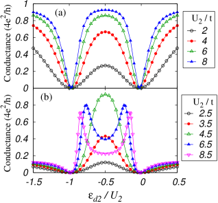
Figure 2: (color online) Conductance vs $\varepsilon_{d2}/U_{2}$ for (a) $\Gamma_{N}=1.0t$ and (b) $\Gamma_{N}=0.2t$, for several side-dot repulsions $U_{2}$. The parameters for QD1 are chosen to be $\varepsilon_{d1}=U_{1}=0$, and $\Delta_{d1}=1.0t$ which is the local SC gap defined by $\Delta_{d1}\equiv\Gamma_{S}$.

We can calculate the conductance at zero temperature as a function of the level position $\varepsilon_{d2}$ of QD2 for different values of $U_{2}$, using the Kubo formula.Izumida In this paper we focus on the Coulomb interaction in the side dot (QD2), assuming that $U_{1}=0$ in the following. The results of the conductance are shown in Fig. 2 for $\varepsilon_{d1}=U_{1}=0$ and $\Delta_{d1}=1.0t$. The coupling to the normal lead is chosen to be (a) $\Gamma_{N}=1.0t$ and (b) $\Gamma_{N}=0.2t$. The conductance is enhanced for the Kondo regime $-U_{2}<\varepsilon_{d2}<0$, where the wide Kondo valley appears in the case of the normal transport. This is a novel phenomenon caused by the interplay between superconductivity and the Kondo effect; the local gap $\Delta_{d1}$ due to the proximity into QD1 leads to the Andreev transport with destructive interference, but the introduction of $U_{2}$ suppresses the SC interference via QD2, which in turn enhances the conductance. Note that the couplings are symmetric $\Gamma_{S}=\Gamma_{N}$ for Fig. 2 (a), and in this particular case the conductance increases with $U_{2}$ for any $\varepsilon_{d2}$, except for the values $\varepsilon_{d2}\simeq-U_{2}$ and $0.0$. Outside of the Kondo regime, the side dot is empty or doubly occupied, and the interference becomes no longer important. When the coupling to the normal lead is small $\Gamma_{N}<1.0t$ as Fig. 2 (b), the conductance in the Kondo regime decreases after the peak reaches the unitary limit $4e^{2}/h$. This behavior can be related to a crossover from short-range to long-range Kondo screening as illustrated in Fig. 1, and is discussed later again.

We examine the behavior at the middle point $\varepsilon_{d2}=-U_{2}/2$ of Fig. 2 in detail. The low-lying energy states show the Fermi-liquid properties, TanakaNQDS and the conductance can be deduced from the renormalized parameters for the quasi-particles (see Eq. (7)).

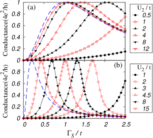
Figure 3: (color online) Conductance vs $\Gamma_{S}/t$ at $\varepsilon_{d2}=-U_{2}/2$ and $\varepsilon_{d1}=U_{1}=0$ for several values of $U_{2}$. (a) $\Gamma_{N}=1.0t$ and (b) $\Gamma_{N}=0.2t$. The dashed line is the conductance of a single dot ($t=0$), for which the horizontal axis should be interpreted as (a) $1.0\Gamma_{S}/\Gamma_{N}$ and (b) $0.2\Gamma_{S}/\Gamma_{N}$.

The conductance is plotted as a function of $\Gamma_{S}/t$ in Fig. 3 for (a) $\Gamma_{N}=1.0t$ and (b) $\Gamma_{N}=0.2t$. We see that the peak shifts towards smaller $\Gamma_{S}$ as $U_{2}$ increases and will coincide in the limit of $U_{2}\to\infty$ with the dashed line, which corresponds to the conductance without the side dot. It means that the interference caused by the side dot is suppressed completely for large $U_{2}$, and in this limit the conductance reaches the unitary limit value for the symmetric couplings $\Gamma_{S}=\Gamma_{N}$. The difference in the line shape of Fig. 2 (a) and that of Fig. 2 (b) at fixed $\Gamma_{S}$ reflects the position of the unitary-limit peak in Fig. 3.

III.2 Fermi-liquid properties at $\varepsilon_{d2}=-U_{2}/2$

In order to clarify the properties of the the ground state precisely, we consider a special case $\varepsilon_{d2}=-U_{2}/2$. Then the Hamiltonian $H^{\mathrm{eff}}$ can be written in terms of the interacting Bogoliubov particles, which conserve the total charge, as shown in Appendix.TanakaNQDS Consequently, the low-energy states can be described by a local Fermi liquid, the fixed-point HamiltonianHewson:qp of which can be written in the form

$$\widetilde{H}_{qp}^{(0)}\ =\ \widetilde{\Delta}_{d2}\left(d_{2\uparrow}^{\dagger}d_{2\downarrow}^{\dagger}+\textrm{H.c.}\right)+\widetilde{t}\,\sum_{\sigma}\left(d_{1\sigma}^{\dagger}d_{2\sigma}+\textrm{H.c.}\right)$$

$$\qquad\quad-\Delta_{d1}\left(d^{{\dagger}}_{1\uparrow}d^{{\dagger}}_{1\downarrow}+\textrm{H.c.}\right)+H_{T,N}+H_{N}.$$ (6)

Here, $\widetilde{\Delta}_{d2}$ is a local SC gap that emerges in QD2 via the self-energy correction due to $U_{2}$, while $\Delta_{d1}\equiv\Gamma_{S}$ as defined in Eq. (5) is caused by the direct proximity from the SC lead. $\widetilde{t}$ is the renormalized value of the inter-dot hopping matrix element. We calculate these parameters from the fixed-point of NRG.Hewson2 Then, the conductance $G$ and a staggered sum $K$ of the pair correlation are deduced from the phase shift, $\theta$, of the Bogoliubov particles,

$$G=\frac{4e^{2}}{h}\,\textrm{sin}^{2}2\theta\;,\qquad K\equiv\sum_{i=1,2}(-1)^{i-1}\,\kappa_{i}=\frac{2\theta}{\pi},$$ (7)

$$\tan\theta\,\equiv\,\frac{\widetilde{\Delta}_{d2}\,\Gamma_{N}}{\widetilde{t}^{2}-\widetilde{\Delta}_{d2}\Gamma_{S}},\qquad\kappa_{i}\equiv\langle d_{i\uparrow}^{\dagger}d_{i\downarrow}^{\dagger}+d_{i\downarrow}d_{i\uparrow}\rangle.$$ (8)

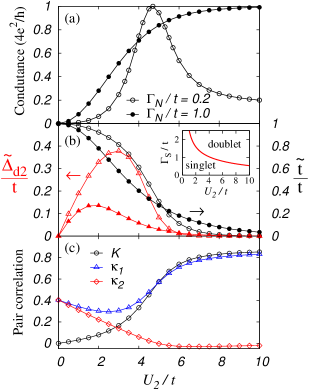
Figure 4: (color online) Ground state properties at $\varepsilon_{d2}=-U_{2}/2$: (a) Conductance, (b) $\widetilde{t}$, $\widetilde{\Delta}_{d2}$, (c) $\kappa_{1}$, $\kappa_{2}$, and $K\equiv\kappa_{1}-\kappa_{2}$. We choose $\varepsilon_{d1}=U_{1}=0$, $\Gamma_{S}=1.0t$, and for filled (open) marks $\Gamma_{N}=1.0t$ ($0.2t$). Inset of (b): Phase boundary, between singlet and doublet ground states, for an isolated DQD ($\Gamma_{N}=0$) with a finite local SC gap $\Delta_{d1}\equiv\Gamma_{S}$.

In Fig. 4, we show the $U_{2}$ dependence of the ground-state properties at $\varepsilon_{d2}=-U_{2}/2$ for $\varepsilon_{d1}=U_{1}=0$ and $\Gamma_{S}=1.0t$. The coupling is chosen to be $\Gamma_{N}=0.2t$, and $1.0t$. The conductance for $\Gamma_{N}<\Gamma_{S}$ shows a peak as a function of $U_{2}$, while for $\Gamma_{N}=\Gamma_{S}$ it increases simply towards the unitary limit. This corresponds to the difference that we see in Fig. 2(a) and (b) at $\varepsilon_{d2}=-U_{2}/2$. Figure 4(b) shows the renormalized parameters ($\circ,\bullet$) $\widetilde{t}$ and ($\vartriangle$,$\blacktriangle$) $\widetilde{\Delta}_{2}$. The ratio $\widetilde{t}/t$, which equals to the square root of the wavefunction renormalization factor $Z$ (see Appendix), decreases monotonically from $1.0$ to $0.0$ with increasing $U_{2}$, while the local SC gap $\widetilde{\Delta}_{d2}$ becomes large for intermediate values of $U_{2}$. The behavior of these Fermi-liquid parameters implies that a crossover from weak to strong correlation regimes occurs around $U_{2}\simeq 4.5t$. The nature of the crossover can be related to a level crossing taking place in a molecule limit $\Gamma_{N}=0$, where QD1 is decoupled from the normal lead. In this limit, the isolated DQD is described by a Hamiltonian $H_{DQD}+H^{\mathrm{eff}}_{S}$, which includes the local SC gap $\Delta_{d1}\equiv\Gamma_{S}$ at QD1. The ground state of the molecule is a singlet or doublet depending on $U_{2}/t$ and $\Gamma_{S}/t$, as shown in the inset of Fig. 4(b). The ground state is a spin-singlet, if either $U_{2}/t$ or $\Gamma_{S}/t$ is small. In the opposite case, a spin-doublet becomes the ground state. The local moment in this doublet state emerges mainly at QD2, because the correlation at QD1 is small in the present situation $\varepsilon_{d1}=U_{1}=0$. We see in the phase diagram in Fig. 4(b) that the transition takes place in this molecule limit at $U_{2}\simeq 4.5t$ for $\Gamma_{S}=1.0t$, and it agrees well with the position where the conductance peak appears in Fig. 4(a).

For finite $\Gamma_{N}$, conduction electrons can tunnel from the normal lead to QD2 via QD1. However, the SC correlation $\Delta_{d1}\equiv\Gamma_{S}$ tends to make the local state at QD1 a singlet, which consists of a linear combination of the empty and doubly occupied states. Thus, for large $\Gamma_{S}$, the electrons at QD1 can not contribute to the screening of the moment at QD2. In this situation, the Kondo screening is achieved mainly by the conduction electrons tunneling to QD2 virtually via QD1. This process is analogous to a superexchange mechanism, which can also be expected from the Hamiltonian written in terms of the Bogoliubov particles (20) in Appendix. From these observations we see that the conductance peak at $U_{2}\simeq 4.5t$ in Fig. 4(a) reflects the crossover from the short-range singlet to long-range one due to the superexchange screening process (see also Fig. 1) for the Bogoliubov particles. Note that the peak structure of the conductance vanishes for $\Gamma_{N}=\Gamma_{S}$.

The deformation of the Kondo cloud can also be deduced from the results shown in Fig. 4(c). This is because the staggered pair correlation $K$ is related directly to the scattering phase shift $\theta$ of the Bogoliubov particles, by the Friedel sum rule Eq. (24) given in Appendix. Therefore, the value of $K$ reflects the changes occurring in the Kondo clouds. Particularly, a sudden change observed in $K$ around $U_{2}\simeq 4.5t$ shows that the phase of the wavefunction shifts by $\Delta\theta\simeq 0.4\pi$ during this change. This also explains the occurring of the crossover from the short-range to long-range screening. We can also calculate each correlation function $\kappa_{i}$ directly with NRG based on the definition. The local SC correlations $\kappa_{1}$ and $\kappa_{2}$ have the same value in the noninteracting case $U_{2}=\varepsilon_{d2}=0$, and thus in this particular limit there is no reduction in the amplitude of the proximity from QD1 to QD2. The Coulomb interaction $U_{2}$ causes the reduction, as both $\kappa_{1}$ and $\kappa_{2}$ decrease for small $U_{2}$ where the ground state is a singlet with a molecule character. For large $U_{2}$, the SC correlation $\kappa_{2}$ almost vanishes in QD2, while $\kappa_{1}$ shows an upturn and approaches the value expected for $t=0$. Therefore, the SC proximity into QD1 is enhanced when the Kondo cloud expands to form a long-range singlet. Then the tunneling current is not interfered much by the local moment at QD2, and flows almost directly without using the path to the side dot.

III.3 Fano line shape for $\varepsilon_{d1}\neq 0$

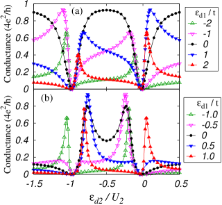
Figure 5: (color online) Conductance vs $\varepsilon_{d2}$ for several values of $\varepsilon_{d1}$, where $U_{1}=0$ and $\Gamma_{S}=1.0t$. Other parameters: (a) $\Gamma_{N}=1.0t$, $U_{2}=8.0t$. (b) $\Gamma_{N}=0.2t$, $U_{2}=6.5t$.

So far, we have chosen the level of QD1 to be $\varepsilon_{d1}=0$. The result obtained for different values of $\varepsilon_{d1}$ is plotted as a function of $\varepsilon_{d2}$ in Fig. 5. We see that two asymmetric Fano structures, each of which consists of a pair of peak and dip, emerge at $\varepsilon_{d2}\simeq 0$ and $-U_{2}$ for $\varepsilon_{d1}\neq 0$, as the Fermi level crosses the energy corresponding to the upper and lower levels of the atomic limit. The conductance peaks become sharper for $\Gamma_{N}<\Gamma_{S}$ as $|\varepsilon_{d1}|$ increases. Maruyama et al studied the Fano structure in the side-coupled DQD system with two normal leads,Maruyama2004 and showed that at low temperatures the conductance has only one pair of the peak and dip, which are separated widely by a Fano-Kondo plateau at $-U_{2}\lesssim\varepsilon_{d2}\lesssim 0$. This type of the plateau was known earlier to appear in a QD embedded in an AB ring.Hofstetter In contrast, our result shows that the Fano-Kondo plateau vanishes, when one of the leads is a superconductor. This is because the Kondo screening in this case is achieved by the long-range singlet bond due to the superexchange process, as a result of the competition between the SC proximity into QD1 and Coulomb interaction at QD2.

IV Summary

We have studied Andreev transport through the side-coupled DQD with NRG approach. We have found that the Coulomb interaction in the side dot suppresses the destructive interference effect typical of the T-shape geometry, and enhances the tunneling current between the normal and SC leads. This novel phenomenon is caused by the interplay between the SC correlation and the Kondo effect; the SC proximity into QD1 pushes the Kondo cloud towards the normal lead, and the conductance shows a peak of the unitary limit as the nature of the singlet changes from a short-range to long-range one. We have also clarified that two asymmetric Fano structures appear in the gate-voltage dependence of the Andreev transport, instead of a reduced single Fano-Kondo plateau which appears in the Kondo regime of the normal transport.

*

Appendix A Bogoliubov particles

The Hamiltonian $H^{\mathrm{eff}}$ defined in Eq. (3) can be transformed, at $\varepsilon_{d2}=-U_{2}/2$, into the interacting Bogoliubov particles, which conserve the total charge. For describing this property briefly, we rewrite $H^{\mathrm{eff}}$ using the logarithmic discretization of NRG,Wilkins

$$\!\!\!\!\mathcal{H}_{\mathrm{NRG}}^{\mathrm{eff}}=\Lambda^{(N-1)/2}\left(H^{\mathrm{eff}}_{S}+H_{DQD}+\mathcal{H}_{T,N}+\mathcal{H}_{N}\right)\,,$$

$$\!\!\!\!\mathcal{H}_{T,N}+\mathcal{H}_{N}=\sum_{n=-1}^{N-1}\sum_{\sigma}t_{n}\Lambda^{-n/2}(f_{n+1\sigma}^{\dagger}f_{n\sigma}^{\phantom{\dagger}}+\textrm{H.c.}).$$ (9)

For $n\geq 0$, the operator $f_{n\sigma}$ describes the conduction electron in the normal lead, and $t_{n}$ is given by

$$\!\!\!\!t_{n}=D\,\frac{1+1/\Lambda}{2}{1-1/\Lambda^{n+1}\over\sqrt{1-1/\Lambda^{2n+1}}\sqrt{1-1/\Lambda^{2n+3}}}\;.$$ (10)

Here, $D$ is the half-width of the conduction band. For the double-dot part, we use a notation $f_{-i,\sigma}=d_{i\sigma}$ for $i=1,2$. Correspondingly, $t_{-1}\equiv\overline{v}\,\Lambda^{-1/2}$ and $t_{-2}\equiv t\,\Lambda^{-1}$ with

$$\!\!\overline{v}=\sqrt{\frac{2\,\Gamma_{N}D\,A_{\Lambda}}{\pi}},\quad\ A_{\Lambda}=\frac{1}{2}\left(\,{1+1/\Lambda\over 1-1/\Lambda}\,\right)\log\Lambda.$$ (11)

At $\xi_{d2}\equiv\varepsilon_{d2}+U_{2}/2=0$, the system has a uniaxial symmetry in the Nambu pseudo-spin space,Yoshihide and the Hamiltonian can be simplified by the transformation

$$\left[\begin{array}[]{c}\gamma_{n\uparrow}^{\phantom{\dagger}}\\ (-1)^{n-1}\gamma_{n\downarrow}^{\dagger}\end{array}\right]=\left[\begin{array}[]{cc}u&-v\\ v&\ u\rule{0.0pt}{14.22636pt}\end{array}\right]\left[\begin{array}[]{c}f_{n\uparrow}^{\phantom{\dagger}}\\ (-1)^{n-1}f_{n\downarrow}^{\dagger}\end{array}\right]\;,$$ (18)

$$u=\sqrt{\frac{1}{2}\left(1+\frac{\xi_{d1}}{E_{d1}}\right)},\quad v=\sqrt{\frac{1}{2}\left(1-\frac{\xi_{d1}}{E_{d1}}\right)}\;.$$ (19)

Here, $\,E_{d1}\equiv\sqrt{\xi_{d1}^{2}+|\Delta_{d1}^{\phantom{*}}|^{2}}$, $\xi_{d1}\equiv\varepsilon_{d1}+U_{1}/2$, and $\Delta_{d1}\equiv\Gamma_{S}$ as defined in Eq. (5). Then $\mathcal{H}_{\mathrm{NRG}}^{\mathrm{eff}}$ is transformed into a normal two-impurity Anderson model for the Bogoliubov particles

$$\!\!\!\mathcal{H}_{\mathrm{NRG}}^{\mathrm{eff}}=\Lambda^{(N-1)/2}\Biggl{[}\,E_{d1}\left(\widehat{n}_{\gamma,-1}-1\right)+\sum_{i=1,2}\frac{U_{i}}{2}\left(\widehat{n}_{\gamma,-i}-1\right)^{2}$$

$$\qquad\quad+\sum_{n=-2}^{N-1}\sum_{\sigma}t_{n}\Lambda^{-n/2}\left(\gamma_{n+1\sigma}^{\dagger}\gamma_{n\sigma}^{\phantom{\dagger}}+\textrm{H.c.}\right)\Biggr{]}.$$ (20)

Here, $\,\widehat{n}_{\gamma i}\equiv\sum_{\sigma}\gamma_{i\sigma}^{\dagger}\gamma_{i\sigma}^{\phantom{\dagger}}$, and the total number of the Bogoliubov particles, $\widehat{Q}_{\gamma}\equiv\sum_{i=-2}^{N}\widehat{n}_{\gamma i}$, is conserved. The equation (20) implies that the low-energy excited states can be described by a local Fermi-liquid theory. This is true also for the original Hamiltonian $H^{\mathrm{eff}}$, and it does not depend on the discretization procedure of NRG.Yoshihide

To be specific, we assume that $U_{1}=0$ in the following. In this case, the Bogoliubov particles feel a normal impurity potential $E_{d,1}$ at QD1, and this potential causes the superexchange mechanism that makes the singlet-bond long range as discussed in Sec. III.2. The retarded Green’s function for the Bogoliubov particle $\gamma_{-2,\sigma}$ at QD2 takes the form

$$G_{\gamma}(\omega)=\frac{1}{\omega-\Sigma_{\gamma}(\omega)-\frac{\displaystyle\mathstrut t^{2}}{\displaystyle\mathstrut\omega-E^{\phantom{0}}_{d1}+i\Gamma_{N}}}\;,$$ (21)

where $\Sigma_{\gamma}(\omega)$ is the self-energy caused by the interaction $(U_{2}/2)\left(\widehat{n}_{\gamma,-2}-1\right)^{2}$. At zero temperature, the asymptotic form of the Green’s function for small $\omega\simeq 0$ is given by

$$G_{\gamma}(\omega)\simeq\frac{Z}{\omega-\widetilde{\Delta}_{d2}-\frac{\displaystyle\mathstrut\widetilde{t}^{\;2}}{\displaystyle\mathstrut\omega-E^{\phantom{0}}_{d1}+i\Gamma_{N}}}\;,$$ (22)

$$\widetilde{\Delta}_{d2}\equiv Z\,\Sigma_{\gamma}(0),\quad\widetilde{t}\equiv\sqrt{Z}\,t,\quad Z^{-1}\!\equiv 1-\left.\!\frac{\partial\Sigma_{\gamma}(\omega)}{\partial\omega}\right|_{\omega=0}.$$ (23)

Note that $\widetilde{\Delta}_{d2}$ has a finite value even though $\xi_{d2}=0$, because $E_{d1}\neq 0$. The value of the parameters $\widetilde{\Delta}_{d2}$ and $\widetilde{t}$ can be deduced from the fixed point of NRG.Hewson2 Then, using the Friedel sum rule for Eq. (20), the local charge at the double dot can be calculated from the phase shift $\theta$ of the Bogoliubov particles,

$$\left\langle\widehat{n}_{\gamma,-2}\right\rangle+\left\langle\widehat{n}_{\gamma,-1}\right\rangle\,=\,\,\frac{2}{\pi}\left(\pi-\theta\right)\;,$$ (24)

$$\qquad\theta\equiv{\rm tan}^{-1}\left(\frac{\widetilde{\Delta}_{d2}\Gamma_{N}}{\widetilde{t}^{2}-\widetilde{\Delta}_{d2}E_{d1}}\right)\,.$$ (25)

The charge of the Bogoliubov particles corresponds to the SC pair correlation for the original electrons $f_{n\sigma}$. Specifically for $\xi_{d1}=0$, it is transformed into the staggered sum $K$ given in Eq. (7), by the inverse transformation of Eq. (18). Similarly, the conductance $G$ can be expressed in terms of the phase shift $\theta$. Furthermore, the free quasi-particles corresponding to the Green’s function given in Eq. (22) can be described by a Hamiltonian, which is rewritten in terms of the original electron operators in Eq. (6) by the inverse transformation.

References

- (1) Present address: Condensed Matter Theory Laboratory, RIKEN, Wako, Saitama 351-0198, Japan
- (2) D. Goldhaber-Gordon, H. Shtrikman, D. Mahalu, D. Abusch-Magder, U. Meirav, and M. A. Kanster, Nature (London) 391, 156 (1998); S. M. Cronenwett, T. H. Oosterkamp, and L. P. Kouwenhoven, Science 281, 540 (1998).
- (3) M. R. Buitelaar, T. Nussbaumer and C. Schönenberger, Phys. Rev. Lett. 89, 256801 (2002).
- (4) A. Eichler, M. Weiss, S. Oberholzer, C. Schönenberger, A. Levy Yeyati, J. C. Cuevas, and A. Martn-Rodero, Phys. Rev. Lett. 99, 126602 (2007).
- (5) T. Sand-Jespersen, J. Paaske, B. M. Andersen, K. Grove-Rasmussen, H. I. Jørgensen, M. Aagesen, C. B. Sørensen, P. E. Lindelof, K. Flensberg, and J. Nygård, Phys. Rev. Lett. 99, 126603 (2007).
- (6) C. Buizert, A. Oiwa, K. Shibata, K. Hirakawa, and S. Tarucha, Phys. Rev. Lett. 99, 136806 (2007).
- (7) K. Grove-Rasmussen, H. I. Jørgensen, and P. E. Lindelof, New J. Phys. 9, 124 (2007).
- (8) J.-P. Cleuziou, W. Wernsdorfer, V. Bouchiat, T. Ondarcuhu, and M. Monthioux, Nature Nanotechnology 1, 53 (2006).
- (9) R. Fazio and R. Raimondi, Phys. Rev. Lett. 80, 2913 (1998); 82, 4950(E) (1999).
- (10) P. Schwab and R. Raimondi, Phys. Rev. B 59, 1637 (1999).
- (11) A. A. Clerk, V. Ambegaokar, and S. Hershfield, Phys. Rev. B 61, 3555 (2000).
- (12) Q.-F. Sun, H. Guo, and T.-H. Lin, Phys. Rev. Lett. 87, 176601 (2001).
- (13) J. C. Cuevas, A. L. Yeyati, and A. Martn-Rodero, Phys. Rev. B 63, 094515 (2001).
- (14) Y. Avishai, A. Golub, and A. D. Zaikin, Phys. Rev. B 63, 134515 (2001); Europhys. Lett. 55, 397 (2001).
- (15) T. Aono, A. Golub, and Y. Avishai, Phys. Rev. B 68, 045312 (2003).
- (16) M. Krawiec and K. I. Wysokiński, Supercond. Sci. Technol. 17, 103 (2004).
- (17) J. Splettstoesser, M. Governale, J. König, F. Taddei, and R. Fazio, Phys. Rev. B 75, 235302 (2007).
- (18) T. Domański, A. Donabidowicz, and K. I. Wysokiński, Phys. Rev. B 76, 104514 (2007).
- (19) A. Golub and Y. Avishai, Phys. Rev. B 69, 165325 (2004).
- (20) Yoichi Tanaka, N. Kawakami, and A. Oguri, J. Phys. Soc. Jpn. 76, 074701 (2007).
- (21) M. R. Gräber, T. Nussbaumer, W. Belzig, and C. Scönenberger, Nanotechnology 15, S479 (2004).
- (22) H. R. Krishna-murthy, J. W. Wilkins, and K. G. Wilson, Phys. Rev. B 21, 1003 (1980); 21, 1044 (1980).
- (23) T.-S. Kim and S. Hershfield, Phys. Rev. B 63, 245326 (2001).
- (24) Y. Takazawa, Y. Imai, and N. Kawakami, J. Phys. Soc. Jpn. 71, 2234 (2002).
- (25) P. S. Cornaglia and D. R. Grempel, Phys. Rev. B 71, 075305 (2005).
- (26) Yoichi Tanaka and N. Kawakami, Phys. Rev. B 72, 085304 (2005).
- (27) R. Žitko and J. Bonča, Phys. Rev. B 73, 035332 (2006).
- (28) C. Karrasch, T. Enss, and V. Meden, Phys. Rev. B 73, 235337 (2006).
- (29) A. Ramšak, J. Mravlje, R. Žitko and J. Bonča, Phys. Rev. B 74, 241305(R) (2006).
- (30) I. Maruyama, N. Shibata, and K. Ueda, J. Phys. Soc. Jpn. 73, 3239 (2004).
- (31) I. Affleck, J. -S. Caux, and A. M. Zagoskin, Phys. Rev. B 62, 1433 (2000).
- (32) A. Oguri, Yoshihide Tanaka, and A. C. Hewson, J. Phys. Soc. Jpn. 73, 2494 (2004).
- (33) W. Izumida, O. Sakai, and Y. Shimizu, J. Phys. Soc. Jpn. 66, 717 (1997).
- (34) A. C. Hewson, A. Oguri, and D. Meyer, Eur. Phys. J. B 40, 177 (2004).
- (35) A. C. Hewson, Phys. Rev. Lett. 70, 4007 (1993); J. Phys.: Condens. Matter 13, 10011 (2001).
- (36) W. Hofstetter, J. König and H. Schoeller, Phys. Rev. Lett. 87, 156803 (2001).
- (37) Yoshihide Tanaka, A. Oguri, and A. C. Hewson, New J. Phys. 9, 115 (2007).