Spin chain model for correlated quantum channels

Abstract

We analyze the quality of the quantum information transmission along a correlated quantum channel by studying the average fidelity between input and output states and the average output purity, giving bounds for the entropy of the channel. Noise correlations in the channel are modeled by the coupling of each channel use with an element of a one dimensional interacting quantum spin chain. Criticality of the environment chain is seen to emerge in the changes of the fidelity and of the purity.

1 Introduction

The common scenario in quantum communication protocols is constituted by two distant parties, Alice and Bob, who want to exchange information through a quantum communication link. Due to unavoidable noise in the channel, this cannot be perfectly accomplished, and some strategies aimed to reduce communication errors have to be employed. These are based on complex encoding/decoding operations and on suitably tailoring the physical system that acts as a channel. In this context the effect of noise on the quantum communication is typically quantified by the so called capacities of the channel, that is the optimal rates at which (quantum or classical) information can be reliably transmitted in the limit of infinite channel uses [1]. The vast majority of the results obtained so far focused on the case of memoryless quantum channels, where the noise acts independently for each channel use. However, in real physical situations, correlations in the noise acting between successive uses can be established. When this happens the communication line is said to be a memory channel, or more precisely, a correlated channel. The analysis of these setups is much more demanding than the memoryless case, and, at present, only a restricted class of them has been solved [2, 3, 4, 5, 6, 8, 9, 7].

Recently, a physical model for representing correlated channels has been proposed in Refs. [4, 10], which, in the context of Bosonic channels and qubit channels respectively, has established a direct connection between these systems and many-body physics. The setup discussed in these proposals is depicted in Fig. 1. Here Alice sends her messages to Bob by encoding them into a $n$-long sequence of information carriers $S$ (the red dots of the figure), which model subsequent channel uses associated with $n$ independent Bosonic modes [4] or $n$ independent spins [10]. The correlated noise of the channel is then described by assuming that each carrier interacts independently with a corresponding element of a $n$-party environment $E$ (sketched with the connected black dots of the figure), which, in Refs. [4] and [10], represents a multi-mode Gaussian state and a many-body spin state, respectively. Thus given an input state $\rho_{S}$ of the $n$ carriers, the corresponding output state associated with the channel is

$${\cal E}_{n}(\rho_{S})=\mbox{Tr}_{E}[{\cal U}\,(\rho_{S}\otimes\sigma_{E})\,{\cal U}^{\dagger}]\;,$$ (1)

where $\sigma_{E}$ is the joint input state of $E$ and the partial trace is performed over the environment. In this equation ${\cal U}$ represents the unitary coupling between $S$ and $E$, which is expressed as

$${\cal U}=\bigotimes_{\ell=1}^{n}U^{(\ell)}\;,$$ (2)

with $U^{(\ell)}$ being the interaction between the $\ell$-th carrier and its environmental counterpart (in Ref. [4] these were beam-splitter couplings, while in Ref. [10] they were phase-gate couplings). Within this framework, memoryless channels ${\cal E}_{n}={\cal E}^{\otimes n}$ are obtained for factorizable environmental input states, while correlated noise models correspond to correlated environmental states $\sigma_{E}$. Interestingly enough, in Ref. [10] it was shown that it is possible to relate the quantum capacity [11] of some specific channels (1) to the properties of the many-body environment $E$.

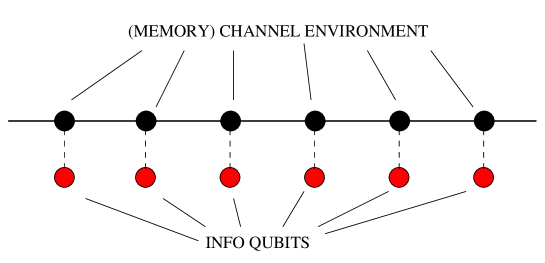
Figure 1: Model for memory channels: The red dots represent the channel uses (ordered, for instance, starting from the left to the right). The channel noise is modeled as a collection of local interactions between the channel uses and the many-body environment $E$ (black dots).

In this paper we discuss a variation of the model (1), which allows us to adapt some of the techniques used in Ref. [12] for characterizing the decoherence effects induced by spin quantum baths, in order to analyze the efficiency of a class of correlated qubits channels. To do so we consider a unitary coupling ${\cal U}$ that does not factorize as in Eq. (2). Instead we assume $E$ to be a spin chain characterized by a free Hamiltonian $\mathcal{H}_{E}$, whose elements interact with the carriers $S$ through the local Hamiltonian $\mathcal{H}_{\rm int}$. With this choice we write

$${\cal U}=\exp[-i\,(\mathcal{H}_{E}+\mathcal{H}_{\rm int})\,t]\;,$$ (3)

with the interaction time $t$ being a free parameter of the model. In particular, as a chain Hamiltonian, we consider a spin-$1/2$ $XY$ model in a transverse field, which can exhibit, in some parameters region, ground state critical properties that greatly enhance spin correlations [13]. Therefore the distance of the chain from criticality is non trivially related to memory effects in the channel. In the second part of the paper, we generalize the previous scheme by introducing a given number of $m$ extra spins between any two consecutive qubits, as shown in Fig. 2. In this case, we can use the number $m$ to modulate the memory effects.

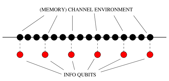
Figure 2: Generalized model of spin chain memory channels. As an example, in this figure we set $m=2$.

2 The Model

As the environment $E$ of the system in Fig. 1 we consider an interacting one-dimensional quantum spin-$1/2$ chain described by an $XY$ exchange Hamiltonian in a transverse magnetic field:

$$\mathcal{H}_{E}=-\frac{J}{2}\sum_{j=1}^{n}\left[(1+\gamma)\sigma_{j}^{x}\sigma_{j+1}^{x}+(1-\gamma)\sigma_{j}^{y}\sigma_{j+1}^{y}+2\lambda\sigma_{j}^{z}\right]\;,$$ (4)

where $\sigma^{\alpha}_{j}$ (with $\alpha=x,y,z$) are the Pauli matrices of the $j$-th spin, $J$ is the coupling strength between neighboring spins, and $\lambda$ is the external field strength . The model in Eq. (4) for $0<\gamma\leq 1$ belongs to the Ising universality class, and has a critical point at $\lambda_{c}=1$; for $\gamma=0$ it reduces to the $XX$ universality class, that is critical for $|\lambda|\leq 1$ [13].

Following Ref. [12], we then assume that each carrier qubit is coupled to one environmental spin element through the coupling Hamiltonian

$$\mathcal{H}_{\rm int}(j)=-\varepsilon|e\rangle_{j}\langle e|\otimes\sigma^{z}_{j}\;,$$ (5)

where $\left|g\right\rangle_{j}$ and $\left|e\right\rangle_{j}$ respectively represent the ground and the excited state of the $j$-th qubit. Hence the total Hamiltonian $\mathcal{H}\equiv\mathcal{H}_{E}+\mathcal{H}_{\rm int}$ is given by

$$\mathcal{H}=-\frac{J}{2}\sum_{j=1}^{n}\left[(1+\gamma)\sigma_{j}^{x}\sigma_{j+1}^{x}+(1-\gamma)\sigma_{j}^{y}\sigma_{j+1}^{y}+2\lambda\sigma_{j}^{z}\right]-\varepsilon\sum_{j=1}^{n}|e\rangle_{j}\langle e|\sigma_{j}^{z}.$$ (6)

Finally, as in Refs. [10, 12], we suppose that at time $t=0$ the environment chain is prepared in the ground state $\left|\varphi\right\rangle_{E}$ of ${\cal H}_{E}$. We then consider a generic input state $\left|\psi\right\rangle_{S}$ of the $n$ qubit carriers of the system (i.e., the input state of the red dots in Fig. 1), and write it in the computational basis:

$$\left|\psi\right\rangle_{S}=\sum_{x}\alpha_{x}\left|x\right\rangle_{S}\,,$$ (7)

where $\alpha_{x}$ are complex probability amplitudes and the sum runs over $N=2^{n}$ possible choices of $x$, each of them being a binary string of $n$ elements in which the $j$-th element is represented as $g$ or $e$, according to the state (ground or excited, respectively) of the corresponding $j$-th qubit.

For each vector $\left|x\right\rangle_{S}$ we define ${\cal S}_{x}$ as the set of the corresponding excited qubits (for instance, given $n=5$ and $\left|x\right\rangle_{S}=\left|egeeg\right\rangle_{S}$, then ${\cal S}_{x}$ contains the $1^{\rm st}$, $3^{\rm rd}$ and $4^{\rm th}$ qubits). After a time $t$, the global state of the qubits and the chain will then evolve into

$$\left|\psi\right\rangle_{S}\otimes\left|\varphi\right\rangle_{E}\quad\stackrel{{\scriptstyle\cal U}}{{\longrightarrow}}\quad\sum_{x}\alpha_{x}\left|x\right\rangle_{S}\otimes{\cal U}_{x}\left|\varphi\right\rangle_{E}\;,$$ (8)

where ${\cal U}$ is the global evolution operator of Eq. (3), while ${\cal U}_{x}\equiv\exp[-i\,\mathcal{H}_{E}^{x}\,t]$ is associated to the following chain Hamiltonian:

$$\mathcal{H}_{E}^{x}\equiv\mathcal{H}_{E}-\varepsilon\sum_{j\in{\cal S}_{x}}\sigma_{j}^{z}\,.$$ (9)

According to Eq. (1), the channel output state is then described by the density matrix

$${\cal E}_{n}(|\psi\rangle_{S}\langle\psi|)=\rho_{S}^{\prime}=\sum_{x,y}L_{xy}\;\alpha_{x}\alpha_{y}^{*}\;|x\rangle_{S}\langle y|\;,$$ (10)

where

$$L_{xy}\equiv{{}_{E}\langle}\varphi|\,{\cal U}_{y}^{\dagger}\,{\cal U}_{x}\left|\varphi\right\rangle_{E}\;,$$ (11)

can be seen as a generalized Loschmidt echo, denoting the scalar product of the input environment state $\left|\varphi\right\rangle_{E}$ evolved with ${\cal U}_{x}$ and ${\cal U}_{y}$, respectively [14]. These quantities can be evaluated by first mapping the Hamiltonian (9) into a free-fermion model via a Jordan Wigner transformation [15]

$$c_{k}=\exp\Bigg{(}i\pi\sum_{j=1}^{k-1}\sigma_{j}^{+}\sigma_{j}^{-}\Bigg{)}\,\sigma_{k}^{-}\;,$$ (12)

where $\sigma^{\pm}=(\sigma^{x}\pm i\sigma^{y})/2$, and then by diagonalizing it with a Bogoliubov rotation of the Jordan Wigner fermions $\{c^{\dagger}_{k},c_{k}\}_{k=1,\ldots,n}$. This allows one to find an explicit expression of the Loschmidt echo in terms of the determinant of a $2n\times 2n$ matrix (see Ref. [12] for details):

$$L_{xy}={{}_{E}\langle}\varphi|e^{i\mathcal{H}_{E}^{x}t}e^{-i\mathcal{H}_{E}^{y}t}|\varphi\rangle_{E}={\rm det}(\mathbb{I}-\rho_{0}+\rho_{0}e^{iH_{x}t}e^{-iH_{y}t})\,,$$ (13)

where $\mathcal{H}_{k}=\sum_{ij}[H_{k}]_{ij}\Psi^{\dagger}_{i}\Psi_{j}$, ${\bf\Psi^{\dagger}}=\left(c_{1}^{\dagger}\ldots c_{N}^{\dagger}\,c_{1}\ldots c_{N}\right)$, and $[\rho_{0}]_{ij}={{}_{E}\langle}\varphi|\Psi_{i}^{\dagger}\Psi_{j}|\varphi\rangle_{E}$ are the two-point correlation functions of the chain.

3 The channel

The echoes (11) provide a complete characterization of the correlated channel ${\cal E}_{n}$. In particular, since $L_{xx}=1$ for all $x$, Eq. (10) shows that the channel ${\cal E}_{n}$ is unital, i.e. it maps the completely mixed state $\frac{1}{N}\sum_{x}|x\rangle_{S}\langle x|$ into itself. Furthermore, the $N\times N$ matrix of elements $L_{xy}/N$ coincides with the Choi-Jamiolkowski state [16] of the map. The latter is defined as the output density matrix obtained when sending through the channel ${\cal E}_{n}$ half of the canonical maximally entangled state $|+\rangle_{SA}\equiv\frac{1}{\sqrt{N}}\sum_{x}|x\rangle_{S}\otimes|x\rangle_{A}$ of the $N$-level system $S$, i.e.

$$J({\cal E}_{n})\equiv({\cal E}_{n}\otimes{\cal I}_{A})(|+\rangle_{SA}\langle+|)=\sum_{x,y}\frac{L_{xy}}{N}\;|xx\rangle_{SA}\langle yy|\;,$$ (14)

with $A$ being a $N$-dimensional ancillary system and ${\cal I}_{A}$ being the identity map. Similarly to the case analyzed in Ref. [10], this is a maximally correlated state [17] whose 1-way distillable entanglement is known to coincides with the “hashing bound” [17, 18, 19]:

$$D_{1}(J({\cal E}_{n}))=H(J_{S}({\cal E}_{n}))-H(J({\cal E}_{n}))=\log_{2}N-H(J({\cal E}_{n}))\;,$$ (15)

where $J_{S}({\cal E}_{n})\equiv\mbox{Tr}_{A}[J({\cal E}_{n})]$ is the reduced density matrix of $J({\cal E}_{n})$ associated with the system $S$, while $H(\cdot)=\mbox{Tr}[(\cdot)\log_{2}(\cdot)]$ is the von Neumann entropy. At least for the subclass of forgetful channels [8], the regularized version of Eq. (15) can then be used [18, 10] to bound the quantum capacity [1, 11] of ${\cal E}_{n}$. This is 

$$Q({\cal E}_{n})\geqslant\lim_{n\rightarrow\infty}\frac{D_{1}(J_{S}({\cal E}_{n}))}{n}=1-\lim_{n\rightarrow\infty}\frac{H(J({\cal E}_{n}))}{n}\;.$$ (16)

The quantity $H(J({\cal E}_{n}))$ corresponds to the entropy of the channel ${\cal E}_{n}$ of Ref. [21], which can be used as an estimator of the channel noise. In our case it has also a simple interpretation in terms of the properties of the many-body system $E$: it measures the entropy of the ground state $|\varphi\rangle_{E}$ after it has evolved through a random application of the perturbed unitaries ${\cal U}_{x}$ , i.e.

$$H(J({\cal E}_{n}))=H(\sigma_{E}^{\prime})\;,\qquad\mbox{with}\qquad\sigma_{E}^{\prime}\equiv\frac{1}{N}\sum_{x}{\cal U}_{x}\;|\varphi\rangle_{E}\langle\varphi|\;{\cal U}^{\dagger}_{x}\;.$$ (17)

Unfortunately, for large $n$ the computation of the von Neumann entropy of the state $J({\cal E}_{n})$ is impractical both analytically and numerically, since it requires to evaluate an exponential number of $L_{xy}$ elements. Interestingly enough, however, we can simplify our analysis by considering the fidelity between $J({\cal E}_{n})$ and its input counterpart $|+\rangle_{SA}$ (see Eq. (14)). As discussed in the following section, this is a relevant information theoretical quantity, since it is directly related to the average fidelity between input and output state of the channel ${\cal E}_{n}$ and provides us an upper bound for $H(J({\cal E}_{n}))$. Similarly we can compute the purity of $J({\cal E}_{n})$ which, on one hand, gives a lower bound for $H(J({\cal E}_{n}))$, while, on the other hand, it is directly related to the average channel output purity of the map ${\cal E}_{n}$.

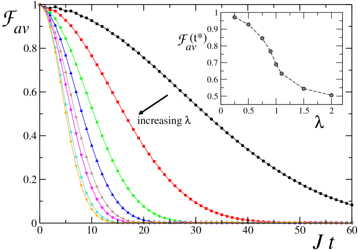
Figure 3: Averaged channel fidelity as a function of the interaction time, for different values of the transverse field $\lambda$: from right to left $\lambda=0.25,\,0.5,\,0.75,\,0.9,\,1,\,1.1,\,1.5,\,2$. Here we simulated a channel of $n=50$ qubits coupled to an Ising chain, and set an interaction strength $\varepsilon=0.05$; the fidelity has been evaluated by sampling over $N_{av}=5\times 10^{4}$ randomly chosen initial conditions. In the inset we plot the averaged fidelity at a fixed interaction time $Jt^{*}=5$, as a function of $\lambda$.

4 Average transmission fidelity

According to Eq. (14), the fidelity between the Choi-Jamiolkowski state $J({\cal E}_{n})$ and its input counterpart coincides with the average value of the Loschmidt echoes $L_{xy}$, i.e.

$${\cal F}\equiv{}_{SA}\langle+|J({\cal E}_{n})|+\rangle_{SA}=\frac{1}{N^{2}}\sum_{x,y}L_{xy}\;.$$ (18)

Even without computing all the $L_{xy}$, this quantity can be numerically evaluated by performing a sampling over $N_{av}$ randomly chosen couples ($x,y$) of initial conditions, and averaging over them :

$${\cal F}\approx{\cal F}_{av}\equiv\frac{1}{N_{av}}\sum_{(x,y)=1}^{N_{av}}{\rm Re}[L_{xy}]\,,$$ (19)

(where we used the fact that $L_{yx}=L_{xy}^{*}$). The quantity ${\cal F}$ provides an upper bound for $H(J({\cal E}_{n}))$ through the quantum Fano inequality [22], i.e.

$$H(J({\cal E}_{n}))\leqslant H_{2}({\cal F})+(1-{\cal F})\log_{2}(4^{n}-1)\leqslant H_{2}({\cal F})+2n(1-{\cal F})\;,$$ (20)

where $H_{2}(\cdot)=-(\cdot)\log_{2}(\cdot)-[1-(\cdot)]\log_{2}[1-(\cdot)]$ is the binary entropy function. Furthermore ${\cal F}$ is directly related to the average transmission fidelity $\langle F\rangle$ of the map ${\cal E}_{n}$. For a given pure input state (7), the transmission fidelity is

$$F(\psi)\equiv{{}_{S}\langle\psi}|{\cal E}_{n}(|\psi\rangle_{S}\langle\psi|)\left|\psi\right\rangle_{S}=\sum_{x,y}L_{xy}|\alpha_{x}|^{2}|\alpha_{y}|^{2}\;.$$ (21)

Taking the average with respect to all possible inputs, we get

$$\langle F\rangle=\sum_{x,y}L_{xy}\,p_{xy}\,,$$ (22)

where $p_{xy}=\langle|\alpha_{x}|^{2}|\alpha_{y}|^{2}\rangle$ with $\langle...\rangle$ being the average with respect to the uniform Haar measure.

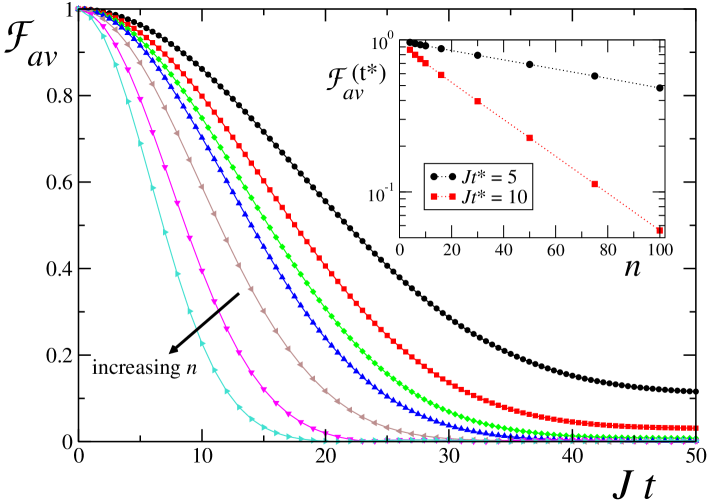
Figure 4: Fidelity for a channel coupled to an Ising chain with $\lambda=1$ and different qubit numbers $n$: from right to left $n=4,\,6,\,8,\,10,\,16,\,30,\,50$; the interaction strength is kept fixed at $\varepsilon=0.05$; data are averaged over $N_{av}=5\times 10^{4}$ configurations. Inset: ${\mathcal{F}}_{av}$ at a fixed time $t^{*}$, as a function of $n$.

The probability distribution $p_{xy}$ can be computed by using simple geometrical arguments [23]. As shown in A, this yields $p_{xy}=\frac{1+2\,\delta_{x,y}}{N(N+2)}$ and hence:

$$\langle F\rangle=\left(\frac{2}{N(N+2)}\sum_{x>y}{\rm Re}[L_{xy}]\right)+\frac{3}{N+2}\,,$$ (23)

where we used the fact that $L_{xx}=1$ and $L_{xy}=L_{yx}^{*}$. Therefore, from Eq. (18) we get

$$\langle F\rangle=\frac{N}{N+2}\;{\cal F}+\frac{2}{N+2}\;.$$ (24)

The fidelities ${\cal F}$ and $\langle F\rangle$ are not directly related to the channel quantum capacity, nonetheless, as in Eq. (20), they can be used to derive bounds for $Q$ . More generally, values near to unity of the fidelity between the output channel states and their corresponding input states, are indicative of a fairly noiseless communication line. On the contrary, values of the transmission fidelities close to zero, while indicating output states nearly orthogonal to their input counterparts, do not necessarily imply null or low capacities, since such huge discrepancies between inputs and outputs could still be corrected by a proper encoding and decoding strategy (e.g. consider the case of a channel which simply rotate the system states).

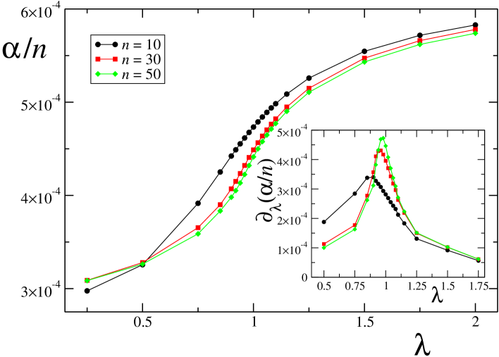
Figure 5: Short-time Gaussian decay rate $\alpha$ as a function of the transverse field $\lambda$. We rescaled $\alpha$ with the system size according to the scaling of Fig. 4. In the inset we plot the first derivative of the same curves in the main panel, with respect to $\lambda$.

Equation (13) allows us to numerically compute the averaged transmission fidelity (19): numerical results in this and in the next sections are given for the case $\gamma=1$, i.e. we study the correlated quantum channel defined by the Ising model. The behavior of the averaged channel fidelity ${\mathcal{F}}_{av}$, defined in Eq. (19) and related to the memory channel scheme of Fig. 1, with respect to the interaction time $t$ (the free model parameter) is shown in Fig. 3: the plots are given for $n=50$ qubits, each of them coupled to one spin of an Ising chain with a coupling strength $\varepsilon=0.05$. Different curves stand for different values of the transverse magnetic field $\lambda$: as it can be clearly seen, the fidelity ${\mathcal{F}}_{av}$ decays as a Gaussian in time, irrespective of the field strength $\lambda$ . The signature of criticality in the environment chain can be identified by studying the function ${\mathcal{F}}_{av}(\lambda,t)$ for fixed interaction time $t^{*}$: the inset of Fig. 3 displays a non analytic behavior for the derivative of ${\mathcal{F}}_{av}(\lambda,t^{*})$ with respect to $\lambda$ at the critical point $\lambda_{c}=1$. This non analyticity will be clearer in the following, where the size scaling will be considered. In Fig. 4 we study the behavior of ${\mathcal{F}}_{av}$ with the number $n$ of qubits, at a fixed value of transverse magnetic field $\lambda=1$. As it is shown in the inset, at a given interaction time $t^{*}$, the fidelity ${\mathcal{F}}_{av}(\lambda_{c},t^{*})$ decays exponentially with $n$ (the same behavior is found when $\lambda\neq 1$). This dependence of the decay rate implies that the average fidelity ${\mathcal{F}}_{av}$ can be fitted by:

$${\mathcal{F}}_{av}\sim e^{-\alpha t^{2}}\qquad\textrm{ with }\quad\alpha\propto n\,;$$ (25)

in other words, the Gaussian decay rate is extensive. Indeed, since the fidelity is a global quantity that describes the evolution of the state of the whole $n$-body system, it should start decaying as a Gaussian (at least at small times) [24], with a reasonably extensive decay ratio. This prediction is confirmed by the results of Fig. 5, where we report the decay rate as a function of the transverse magnetic field for different system sizes $n$. In proximity of the critical point, the decay rate undergoes a sudden change, which becomes more evident when increasing the system size. The signature of criticality at $\lambda_{c}=1$ and the finite size effects can be better analyzed by looking at the derivative of the decay rate with respect to the transverse field: The inset of Fig. 5 clearly show that $\partial_{\lambda}\alpha$ exhibits a non analytic behavior at the critical point $\lambda_{c}$, at the thermodynamical limit. Notice also that, due to finite size effects, the maximum of $\partial_{\lambda}\alpha$ does not coincide exactly with the critical point, that can be rigorously defined only at the thermodynamical limit, but occurs at a slightly smaller value of $\lambda$. However, we checked that a finite size scaling gives the right prediction of the critical point located at $\lambda=1$.

5 Average output purity

Another quantity that can be evaluated with relatively little numerical effort is the purity of the Choi-Jamiolkowski state $J({\cal E}_{n})$, i.e.

$${\cal P}_{2}\equiv\mbox{Tr}[J({\cal E}_{n})^{2}]=\frac{1}{N^{2}}\sum_{xy}|L_{xy}|^{2}\;.$$ (26)

As in the case of ${\cal F}$, this can be computed by approximating the summation with a random sampling, i.e.

$${\cal P}_{2}\approx{\cal P}_{av}\equiv\frac{1}{N_{av}}\sum_{(x,y)=1}^{N_{av}}|L_{xy}|^{2}\,.$$ (27)

The quantity (26) provides us two important pieces of information. First of all, it yields a useful bound on the channel entropy $H(J({\cal E}_{n}))$. This follows from the inequality [25]

$$H(J({\cal E}_{n}))\geqslant H_{2}(J({\cal E}_{n}))=-\log_{2}{\cal P}_{2}\;,$$ (28)

with $H_{2}(\cdot)\equiv-\log_{2}\mbox{Tr}[(\cdot)^{2}]$ being the Rényi entropy of order 2. Furthermore ${\cal P}_{2}$ is directly related to the average output purity $\langle P_{2}\rangle$ of the channel ${\cal E}_{n}$. This is obtained by averaging over all possible inputs $|\psi\rangle_{S}$ the purity of the output state ${\cal E}_{n}(|\psi\rangle_{S}\langle\psi|)$, i.e.

$$\langle P_{2}\rangle\equiv\langle{\rm Tr}\left[({\cal E}_{n}(|\psi\rangle_{S}\langle\psi|))^{2}\right]\rangle=\sum_{x,y}|L_{xy}|^{2}\,\langle|\alpha_{x}|^{2}|\alpha_{y}|^{2}\rangle=\sum_{x,y}|L_{xy}|^{2}\,p_{xy}\,,$$ (29)

where we used Eq. (10) and where $p_{xy}$ are the probabilities defined in Eq. (32). According to Eq. (26) this yields,

$$\langle P_{2}\rangle=\frac{N}{N+2}{\cal P}_{2}+\frac{2}{N+2}\;.$$ (30)

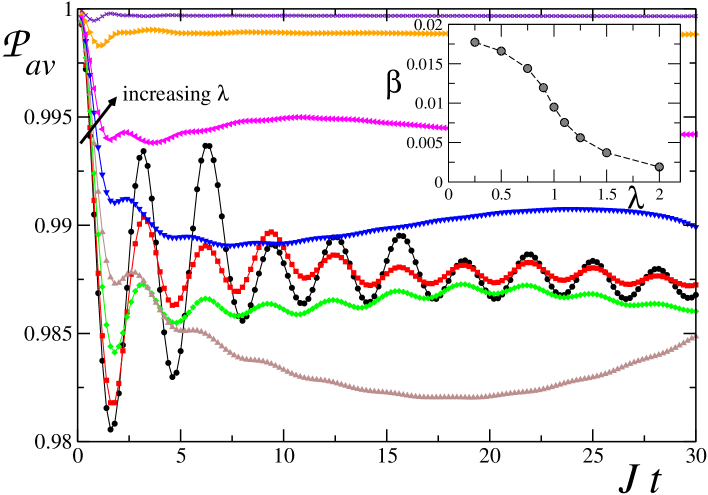
Figure 6: Averaged purity of the channel output state as a function of the interaction time, for various transverse field strengths: from left to right $\lambda=0.25$ (black circles), 0.5 (red squares), 0.75 (green diamonds), 0.9 (brown triangles up), 1 (blue triangles down), 1.1 (magenta triangles left), 1.5 (orange triangles right), 2 (violet crosses). Here we simulated a channel of $n=30$ qubits coupled to an Ising chain, set an interaction strength $\varepsilon=0.05$, and averaged over $N_{av}=5\times 10^{4}$ random initial conditions. In the inset we plot the short-time Gaussian decay rate $\beta$ as a function of $\lambda$.

The average purity is a rather fair indicator of the noise induced by the coupling to the environment: if the carrier qubits get strongly entangled with the environment, $P_{2}$ is greatly reduced from the unit value (for large $n$ it will tend to zero); on the other hand, a channel which simply unitarily rotates the carrier states has a unit purity. However, we should stress that also the purity may intrinsically fail as a transmission quality quantifier: there are strongly noisy channels with very high output purity (consider, for example, the channel which maps each input state into the same pure output state).

Then, we study the average channel purity ${\mathcal{P}}_{av}$ as a function of the model free parameter, the interaction time $t$. The results are reported in Fig. 6 for a chain of $n=30$ qubits and different values of the transverse field $\lambda$. We notice qualitatively different behaviors depending on the values of the transverse field $\lambda$: If $\lambda<\lambda_{c}$ the averaged purity oscillates in time and asymptotically tends to an average constant value; as far as the critical point is approached, ${\mathcal{P}}_{av}$ drops to smaller values (revivals are again due to finite system size effects), reflecting the fact that at criticality correlations between the qubits and the environment are stronger. Crossing the critical point, in the $z$-ordered phase ($\lambda>\lambda_{c}$) the purity is generally higher and asymptotically takes values very close to the unit value. This can be easily understood in the limit $\lambda\to\infty$: in this case the spins in the chain are “freezed” along the field direction and they cannot couple with anything else, resulting in a watchdog-like effect [24]. Independently of the transverse field value, the average purity ${\mathcal{P}}_{av}$ decays as a Gaussian ${\mathcal{P}}_{av}\sim e^{-\beta t^{2}}$ in the short time limit. As for the averaged fidelity ${\mathcal{F}}_{av}$, we have then analyzed the decay rate $\beta$ as a function of $\lambda$: as before, $\beta$ exhibits a signature of criticality via a divergence, at the thermodynamical limit, in its first derivative with respect to $\lambda$ (see the inset of Fig. 6).

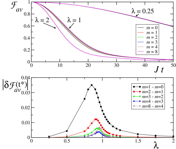
Figure 7: Upper panel: average channel fidelity for the generalized model in Fig. 2, with $n=12$ qubits, $\varepsilon=0.05$ (averages have been performed over $N_{av}=10^{4}$ initial states). The various curves are for different numbers $m$ of spins between two consecutive qubits, and different values of transverse magnetic fields $\lambda=0.25,\,1,\,2$. Lower panel: absolute differences in the fidelities between configurations at various $m$, as a function of $\lambda$ and at a fixed interaction time $Jt^{*}=10$.

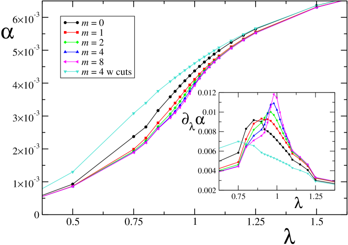
Figure 8: Gaussian decay rate of the averaged fidelity for model in Fig. 2, as a function of the transverse field $\lambda$. The various curves stand for different numbers of spins $m$ between two consecutive qubits (here $n=12$, $\varepsilon=0.05$, $N_{av}=10^{4}$). In the inset we show the first derivative with respect to $\lambda$ of the curves in the main panel.

6 Generalized model

We finally concentrate on the generalized model depicted in Fig. 2, where a certain number $m$ of environment spins are present between two consecutive spins coupled to the qubits. The richness of the model, that is characterized by a large number of parameters, and by a global size which grows both with $n$ and $m$, requires a huge numerical effort in order to simulate it, therefore we decided to analyze only the average channel fidelity ${\mathcal{F}}_{av}$. In the upper panel of Fig. 7 we show ${\mathcal{F}}_{av}$ as a function of the interaction time $t$ for different values of $m$ and three values of the transverse field $\lambda=0.25,\,1,\,2$; we fix a number of qubits $n=12$ and an interaction strength $\varepsilon=0.05$. Hereafter we will concentrate on this case as a typical result, as we performed some checks with larger numbers of channel uses ($n=30,\,50$ and $m=0,\,1,\,2$), and found qualitatively analogous results. We immediately observe that differences for various $m$ are tiny, even if the fidelity generally tends to increase when increasing $m$; the sensibility with $m$ suddenly enhances at criticality ($\lambda_{c}=1$), where correlations in the environment decay much slower than in the other cases. On the other hand, when $\lambda$ is far from $\lambda_{c}$, differences between fidelities upon a variation of $m$ are greatly suppressed, and the generalized model mostly behaves as the model in Fig. 1. Again, this reflects the fact that, out of criticality, each qubit is mostly influenced only by the spin that is coupled to, as the spin does not exchange correlations with the other environmental spins. The resulting channel properties are then defined only by the local properties of the chain. On the contrary, at criticality, the spins are correlated and then the resulting channel properties are influenced by the distance of the spins coupled with the qubits. In the lower panel of Fig. 7 we explicitly plot the differences in the fidelities for various $m$ as a function of $\lambda$, and for a fixed interaction time; a peak in proximity of $\lambda_{c}$ is clearly visible. We point out that, as already noted at the end of Sec. 4 concerning the size scaling of the fidelity, the maximum in the differences does not occur exactly at the critical point.

The sensitivity to criticality is again demonstrated by the averaged fidelity Gaussian decay rate $\alpha$ as a function of $\lambda$, as shown in Fig. 8 for different values of $m$: the first derivative in the inset has a maximum in correspondence of a value that approaches the critical point $\lambda_{c}$ at the thermodynamical limit. Indeed, increasing $m$ is equivalent to approaching the thermodynamical limit of the chain, thus resulting in an increase of the quantum phase transition effects. A double check of this comes from the cyan triangles-down curve of Fig. 8: in this case we take $m=4$, but we break one of the links between two intermediate spins. The environment is then formed by disconnected chains, each of them made up by $5$ spins, therefore the system cannot undergo a phase transition in the limit $n\to\infty$: the signature of criticality has completely disappeared.

7 Conclusions

In conclusion we have introduced and characterized a class of correlated quantum channels, and we have given bounds for its entropy by means of the averaged channel fidelity ${\mathcal{F}}_{av}$ and purity ${\mathcal{P}}_{av}$. Even though in general these bounds might not be strict, we give a characterization of the channel in terms of quantities that have a clear meaning from the point of view of the many body model we have introduced.

In the case of an environment defined by a quantum Ising chain, we have shown that the averaged channel purity and the fidelity depend on the environment parameters and are strongly influenced by spin correlations inside it, in particular by the fact whether the environment is critical or not. We expect that some different environment models, such as, for example, the $XY$ spin chain, will behave qualitatively similarly of what found in this work, as it belongs to the same universality class. This might not be the case for other models, like the Heisenberg chain, which will be object of further study in the near future.

Appendix A

The probability $p_{xy}$ of Eq. (22) can be computed as follows: we first define $r_{x}\equiv|\alpha_{x}|$ and convert the string $x$ into a decimal number from $1$ to $N=2^{n}$ by trivially identifying $g\equiv 0$ and $e\equiv 1$. The average over a uniform distribution of all pure input states on the Bloch hypersphere for $n$ qubits is

$$p_{xy}=C_{N}\int_{0}^{1}{\rm d}r_{1}\cdots\int_{0}^{1}{\rm d}r_{N}\>r_{x}^{2}\,r_{y}^{2}\,\delta(1-{\bf r}^{2})\,,$$ (31)

where ${\bf r}^{2}=r_{1}^{2}+\cdots+r_{N}^{2}$, and $C_{N}^{-1}\equiv\int_{0}^{1}{\rm d}r_{1}\cdots\int_{0}^{1}{\rm d}r_{N}\,\delta(1-{\bf r}^{2})$ is a normalization constant. Changing the limits of integration due to the delta function and using the property of the Gamma function $\Gamma(z)=\int_{0}^{+\infty}y^{z-1}e^{-y}{\rm d}y$, it is easy to show that $C_{N}=2^{N}\pi^{-N/2}\Gamma(N/2)$ and

$$p_{xy}=\frac{1+2\,\delta_{x,y}}{N(N+2)}\,.$$ (32)

Appendix B

For times longer than those in the scales of Figs. 3 and 4, time revivals of the fidelity are present, i.e. the fidelity increases back towards the unit value periodically, due to the finite system size. For finite values of the transverse field revivals are not perfect, that is ${\mathcal{F}}_{av}(t)\neq 1$ for $t>0$. Anyway, as far as $\lambda$ increases, the revivals are stronger and happen with period $t^{R}$ which does not depends on the system size $n$. This can be understood in the limit $\lambda\to+\infty$, where the ground state of the environment $\left|\varphi\right\rangle_{E}$ is a fully $z$-polarized state, thus being an eigenstate of the chain Hamiltonian $\mathcal{H}^{x}_{E}$ in Eq. (9): the generalized Loschmidt echo of Eq. (11) is then given by $L_{xy}=e^{-i\varepsilon\mathcal{N}_{x-y}t}$, where $\mathcal{N}_{x-y}$ is the number of excited qubits in the sequence $x$ minus the one in the sequence $y$. It is easy to see that there are $2^{n}\times{n\choose k}$ different possibilities to choose two sequences $x,y$ such that the corresponding states differ in the state of $k$ qubits, then $\mathcal{N}_{x-y}=\pm j$ with $j=0,2,\ldots,k$ (if $k$ is even) or $j=1,3,\ldots,k$ (if $k$ is odd). Therefore, when averaging over input states, each term contributes with $p_{xy}\,e^{\pm i\,\varepsilon jt}$. Noting that $({\cal U}_{y}^{\dagger}\,{\cal U}_{x})^{\dagger}={\cal U}_{x}^{\dagger}\,{\cal U}_{y}$, we have

$$\langle F\rangle=2^{n}p_{xx}+p_{xy}\left(c_{0}+c_{1}\cos(\varepsilon t)+c_{2}\cos(2\varepsilon t)+\ldots+c_{n}\cos(n\varepsilon t)\right)\;,$$ (33)

It follows a perfect revival for the fidelity at times $t^{R}$ such that $\varepsilon t^{R}=2\pi\;[{\rm mod}\;2\pi].$

References

References

- [1] Bennett C H and Shor P W 1998 IEEE Trans. Inf. Th. 44 2724
-
[2]
Macchiavello C and Palma G M
2002 Phys. Rev. A 65 050301(R);
Macchiavello C, Palma G M, and Virmani S 2004 Phys. Rev. A 69 010303(R) - [3] Bowen G and Mancini S 2004 Phys. Rev. A 69 012306
- [4] Giovannetti V and Mancini S 2005 Phys. Rev. A 71 062304
- [5] Giovannetti V 2005 J. Phys. A 38 10989
- [6] Daems D 2007 Phys. Rev. A 76 021310
- [7] Caruso F, Giovannetti V, Macchiavello C, Ruskai M B 2008 Phys. Rev. A 77 052323
- [8] Kretschmann D and Werner R F 2005 Phys. Rev. A 72 062323
- [9] D’Arrigo A, Benenti G, and Falci G 2007 New J. Phys. 9 310
-
[10]
Plenio M B and Virmani S
2007 Phys. Rev. Lett. 99 120504;
2008 New J. Phys. 10 043032 -
[11]
Lloyd S 1997 Phys. Rev. A 55 1613;
Barnum H, Nielsen M A, and Schumacher B 1998 Phys. Rev. A 57 4153;
Devetak I 2005 IEEE Trans. Inf. Theory 51 44 - [12] Rossini D, Calarco T, Giovannetti V, Montangero S and Fazio R 2007 Phys. Rev. A 75 032333; 2007 J. Phys. A: Math. Theor. 40 8033
- [13] Sachdev S 2000 Quantum Phase Transitions (Cambridge University Press, Cambridge)
- [14] Gorin T, Prosen T, Seligman T H and Žnidarič M 2006 Phys. Rep. 435 33
-
[15]
Lieb E, Schultz T and Mattis D
1961 Ann. Phys. 16 407;
Pfeuty P 1970 Ann. Phys. 57 79 - [16] Bengstsson I and Życzkowski K 2006 Geometry of Quantum States (Cambridge Univ. Press, Cambridge)
-
[17]
Rains E M 1999 Phys. Rev A 60 179;
2001 IEEE Trans. Inf. Th. 47 2921 - [18] Bennett CH, DiVincenzo D P, Smolin J A, and Wootter W K 1999 Phys. Rev. A 54 3824
- [19] Devetak I and Winter A 2005 Proc. R. Soc. Lond. A 461 207.
- [20] Giovannetti V 2005 Phys. Rev. A 71 062332
- [21] Roga W, Fannes M, and Życzkowski K 2008 J. Phys. A: Math. Theor. 41 035305
- [22] Nielsen M A and Chuang I L 2000 Quantum Computation and Quantum Information (Cambridge Univ. Press, Cambridge)
-
[23]
Lubkin E
1978 J. Math. Phys. 19 1028;
Page D N 1993 Phys. Rev. Lett. 71 1291 - [24] Peres A 1995 Quantum Theory: concepts and Methods (Kluwer Academic Publishers, Dordrecht)
- [25] Rényi A 1961 On measures of entropy and information Proc. 4th Berkeley Sympos. Math. Statist. and Prob. Vol. I 547 (Univ. California Press, Berkeley)