Kink structure in the electronic dispersion of high-$T_{\mathrm{c}}$ superconductors from the electron-phonon interaction

Abstract

We investigate the electronic dispersion of high-$T_{\mathrm{c}}$ superconductor on the basis of the two-dimensional three-band Hubbard model with the electron-phonon interaction together with the strong electron-electron interaction. In our model, it is shown across the hole-doped region of high-$T_{\mathrm{c}}$ superconductor that the electron-phonon interaction makes a dispersion kink, observed along the nodal direction, and that the small isotope effect appears on the electronic dispersion.

INTRODUCTION

For the past two decades, extensive studies of high-$T_{\mathrm{c}}$ cuprates have spotlighted many curious phenomena. It has been argued that most phenomena are attributable to the strong correlations among electrons, which play significant roles in these materials. However, since the discovery of sudden changes in the electron dispersion or “kinks” shown by the angle-resolved photoemission spectroscopy (ARPES), Kaminski01 ; Lanzara01 effects of electron-boson interactions on electronic self-energies have been recognized. While the kinks are now indisputable in cuprates, Zhou03 their origin as arising from electronic coupling to phonons ZXShen02 or magnetic excitations Terashima06 ; Zabolotnyy06 ; Kordyuk06 remains unclear.

Recent scanning tunneling microscope study showed that the statistical distribution of energy of bosonic modes ($\Omega$) has meaningful difference between ${}^{16}{\mathrm{O}}$ and ${}^{18}{\mathrm{O}}$ materials. Thus, it should be hard to exclude the possibility that electron-phonon interaction (EPI) significantly affects the electronic states in cuprates.

In this study, we investigate the analysis upon the EPI together with the electron-electron interaction (EEI) on the basis of the two-dimensional (2D) three-band Hubbard–Holstein (HH) model. With the use of our three-band HH model, we can reproduce the situation of the real high-$T_{\mathrm{c}}$ materials, in which EPI mainly works on $p$ electrons at O sites.

FORMULATION

Our model Hamiltonian $H$ is composed of $d$ electrons at each Cu site, $p$ electrons at O site, and lattice vibrations of O atoms. We consider only the on-site Coulomb repulsion $U$ between $d$ electrons at each Cu site as our EEI. Let us define that $\mu$ and $N_{0}$ represent the chemical potential and the number of all electrons, respectively. Then, $H-\mu N_{0}$ is divided into the non-interacting part, $H_{0}$, the electron-electron interacting part $H_{\mathrm{el-el}}$, the phonon part $H_{\mathrm{ph}}$, and the electron-phonon interacting part $H_{\mathrm{el-ph}}$ as

$$H-\mu N_{0} = H_{0}+H_{el-el}+H_{ph}+H_{el-ph},$$

$$N_{0} = \sum_{{\mathbf{k}}\sigma}(d_{{\mathbf{k}}\sigma}^{\dagger}d_{{\mathbf{k}}\sigma}+p_{{\mathbf{k}}\sigma}^{x\dagger}p_{{\mathbf{k}}\sigma}^{x}+p_{{\mathbf{k}}\sigma}^{y\dagger}p_{{\mathbf{k}}\sigma}^{y}).$$ (1)

Here, $d_{{\mathbf{k}}\sigma}(d_{{\mathbf{k}}\sigma}^{\dagger})$ and $p_{{\mathbf{k}}\sigma}^{x(y)}(p_{{\mathbf{k}}\sigma}^{x(y)\dagger})$ are the annihilation (creation) operator for $d$ and $p^{x(y)}$ electrons of momentum ${\mathbf{k}}$ and spin $\sigma$, respectively. The non-interacting part $H_{0}$ is represented by

$$H_{0} = \sum_{{\mathbf{k}}\sigma}\left(d_{{\mathbf{k}}\sigma}^{\dagger}\,p_{{\mathbf{k}}\sigma}^{x\dagger}\,p_{{\mathbf{k}}\sigma}^{y\dagger}\right)\left(\begin{array}[]{ccc}\Delta_{dp}&\zeta_{\mathbf{k}}^{x}&\zeta_{\mathbf{k}}^{y}\\ -\zeta_{\mathbf{k}}^{x}&0&\zeta_{\mathbf{k}}^{p}\\ -\zeta_{\mathbf{k}}^{y}&\zeta_{\mathbf{k}}^{p}&0\\ \end{array}\right)\!\left(\begin{array}[]{c}d_{{\mathbf{k}}\sigma}\\ p_{{\mathbf{k}}\sigma}^{x}\\ p_{{\mathbf{k}}\sigma}^{y}\\ \end{array}\right)$$ (8)

$$\equiv {\sum_{{\mathbf{k}}\sigma}}\mathbf{d}_{{\mathbf{k}}\sigma}^{\dagger}\,\mathbf{H}_{0}\,\mathbf{d}_{{\mathbf{k}}\sigma}.$$ (9)

We take the lattice constant of the square lattice formed from Cu sites as the unit of length. Then, $\zeta_{\mathbf{k}}^{x(y)}=2{\rm i}\,t_{dp}\sin\frac{k_{x(y)}}{2}$ and $\zeta_{\mathbf{k}}^{p}=-4t_{pp}\sin\frac{k_{x}}{2}\sin\frac{k_{y}}{2}$, where $t_{dp}$ is the transfer energy between a $d$ orbital and a neighboring $p^{x(y)}$ orbital and $t_{pp}$ is that between a $p^{x}$ orbital and a $p^{y}$ orbital. $\Delta_{dp}$ is the difference of energy levels of $d$ and $p$ orbitals. In this study, we take $t_{dp}$ as the unit of energy. The residual parts are described as follows:

$$H_{el-el}=\frac{U}{N}\sum_{{\mathbf{k}}{\mathbf{k}}^{\prime}}\sum_{{\mathbf{q}}(\neq{\mathbf{0}})}d_{{\mathbf{k}}+{\mathbf{q}}\uparrow}^{\dagger}d_{{\mathbf{k}}^{\prime}-{\mathbf{q}}\downarrow}^{\dagger}d_{{\mathbf{k}}^{\prime}\downarrow}d_{{\mathbf{k}}\uparrow},$$ (10)

$$H_{ph}=\sum_{{\mathbf{q}}}\!\sum_{\nu=\{x,y\}}\omega^{\nu}_{{\mathbf{q}}}\,b^{\nu\dagger}_{{\mathbf{q}}}b^{\nu}_{{\mathbf{q}}},$$ (11)

and

$$H_{el-ph}=\frac{1}{N}\sum_{{\mathbf{k}}\sigma}\hskip 4.0pt\sum_{{\mathbf{q}}}\!\sum_{\nu=\{x,y\}}g\,\alpha^{\nu}_{\mathbf{k},\mathbf{q}}\,p^{\nu\dagger}_{{\mathbf{k}}+{\mathbf{q}}\sigma}p^{\nu}_{{\mathbf{k}}\sigma}\left(b^{\nu}_{{\mathbf{q}}}+b^{\nu\dagger}_{-{\mathbf{q}}}\right),$$ (12)

where $U$ is the on-site Coulomb repulsion between $d$ orbitals, $N$ is the number of ${\mathbf{k}}$-space lattice points in the first Brillouin zone (FBZ), and $g\,\alpha^{\nu}_{\mathbf{k},\mathbf{q}}\,(\nu=\{x,y\})$ is the electron-phonon matrix element, respectively. We consider that the half-breathing phonon mode, McQueeney01 in which oxygen ions are vibrating along the $x$ or $y$ directions, is crucial for our problem. Thus, ignoring the other phonon modes, we have the electron-phonon interacting part as Eq. (12).

Then, we introduced the unperturbed and perturbed Green’s functions, which are to be described in $3\times 3$ matrix form. The unperturbed Green’s function $\mathbf{G}^{(0)}(\mathbf{k},z)$ is derived from Eq. (9) as

$$\mathbf{G}^{(0)}(\mathbf{k},z)=\left[z\mathbf{I}-\mathbf{H}_{0}\right]^{-1},$$ (13)

where $\mathbf{I}$ is a $3\times 3$ unit matrix. Using the abbreviation of Fermion Matsubara frequencies, $\epsilon_{n}=\pi T(2n+1)$ with integer $n$ and temperature $T$, the perturbed Green function $\mathbf{G}(\mathbf{k},z)$ is determined by the Dyson equation:

$$\mathbf{G}(\mathbf{k},\mathrm{i}\epsilon_{n})\,^{-1}=\mathbf{G}^{(0)}(\mathbf{k},\mathrm{i}\epsilon_{n})\,^{-1}-\mathbf{\Sigma}(\mathbf{k},\mathrm{i}\epsilon_{n}),$$ (14)

where $\mathbf{\Sigma}(\mathbf{k},\mathrm{i}\epsilon_{n})$ is the self-energy expected to be a diagonal matrix. In order to estimate the $d$ electron self-energy $\Sigma_{d}(\mathbf{k},\mathrm{i}\epsilon_{n})\equiv\Sigma_{11}(\mathbf{k},\mathrm{i}\epsilon_{n})$ in Eq. (14), we adopt the fluctuation exchange approximation Bickers89 as follows:

$$\Sigma_{d}(\mathbf{k},\mathrm{i}\epsilon_{n})=\frac{T}{N}\sum_{\mathbf{q}\,m}G_{d}(\mathbf{k}-\mathbf{q},\mathrm{i}\epsilon_{n}-\mathrm{i}\omega_{m})\,V_{\mathrm{el-el}}(\mathbf{q},\mathrm{i}\omega_{m}),$$ (15)

where $G_{d}(\mathbf{k},\mathrm{i}\epsilon_{n})\equiv G_{11}(\mathbf{k},\mathrm{i}\epsilon_{n})$,

$$V_{\mathrm{el-el}}(\mathbf{q},\mathrm{i}\omega_{m}) = \frac{3}{2}\frac{U^{2}\chi(\mathbf{q},\mathrm{i}\omega_{m})}{1-U\chi(\mathbf{q},\mathrm{i}\omega_{m})}+\frac{1}{2}\frac{U^{2}\chi(\mathbf{q},\mathrm{i}\omega_{m})}{1+U\chi(\mathbf{q},\mathrm{i}\omega_{m})}$$ (16)

$$-U^{2}\chi(\mathbf{q},\mathrm{i}\omega_{m}),$$

where $\omega_{m}=2m\,\pi T$ with integer $m$ are Boson Matsubara frequencies, and

$$\chi(\mathbf{q},\mathrm{i}\omega_{m})=-\frac{T}{N}\sum_{\mathbf{k}\,n}G_{d}(\mathbf{q}+\mathbf{k},\mathrm{i}\omega_{m}+\mathrm{i}\epsilon_{n})\,G_{d}(\mathbf{k},\mathrm{i}\epsilon_{n}).$$ (17)

In order to estimate the p^x(y)-electron self-energy $\Sigma_{x(y)}(\mathbf{k},\mathrm{i}\epsilon_{n})\equiv\Sigma_{22(33)}(\mathbf{k},\mathrm{i}\epsilon_{n})$ in Eq. (14), we exploit the Brillouin-Wigner perturbation theory. We adopt the self-consistent one-loop approximation as follows:

$$\Sigma_{x(y)}(\mathbf{k},\mathrm{i}\epsilon_{n})=\frac{T}{N}\sum_{\mathbf{q}\,m}G_{x(y)}(\mathbf{k}-\mathbf{q},\mathrm{i}\epsilon_{n}-\mathrm{i}\omega_{m})\,V_{\mathrm{el-ph}}^{x(y)}(\mathbf{q},\mathrm{i}\omega_{m}),$$ (18)

where $G_{x(y)}(\mathbf{k},\mathrm{i}\epsilon_{n})\equiv G_{22(33)}(\mathbf{k},\mathrm{i}\epsilon_{n})$ and $V_{\mathrm{el-ph}}^{x(y)}(\mathbf{q},\mathrm{i}\omega_{m})$ is the EPI on p^x(y) electron. Our EPI is determined as follows:

$$V_{\mathrm{el-ph}}^{x(y)}(\mathbf{q},\mathrm{i}\omega_{m})=\lambda\left|\alpha^{x(y)}_{\mathbf{q}}\right|^{\,2}\left[\frac{1}{\omega_{\mathrm{h}}+\mathrm{i}\omega_{m}}+\frac{1}{\omega_{\mathrm{h}}-\mathrm{i}\omega_{m}}\right],$$ (19)

where $\lambda=g^{2}/(2\omega_{\mathrm{h}})$ and $\alpha^{x(y)}_{\mathbf{q}}=\sin\frac{q_{x(y)}}{2}$. $\omega_{\mathrm{h}}$ is the specific phonon energy for the half-breathing mode. As above, we ignore the effects in which EEI and EPI are coupled. Thus, as shown by Eqs. (15)-(19), in our formulation, EEI and EPI are completely decoupled. Of course, this assumption is inadequate to analyze the case in which the characteristic energy due to EEI is comparable to the phonon energy. However, as will be seen later, we actually treat the cases with rather high characteristic energy due to EEI. Hence, decoupling EEI with EPI should be justified in our analysis. The electron-phonon coupling constant $\lambda$ does not depend on $M_{\mathrm{O}}$ since $\omega_{\mathrm{h}}\propto M_{\mathrm{O}}^{-1/2}$ and $g\propto\left(M_{\mathrm{O}}\omega_{\mathrm{h}}\right)^{-1/2}$, where $M_{\mathrm{O}}$ is the mass of an oxygen ion. In our model, thus, the isotope effect is reflected on the phonon energy in the electronic self-energies only, but not any changes in the strength.

RESULTS AND DISCUSSION

We need to solve Eqs. (14)–(18) in a fully self-consistent manner. During numerical calculations, we divide the FBZ into $128\times 128$ meshes. We prepare $2^{12}=4096$ Matsubara frequencies for temperature $T\sim 87{\mathrm{K}}$. As shown later, at this temperature, our calculation can reproduce the important behavior of electrons in normal state. Moreover, to our knowledge, the situation will not be changed if we change $T$ to some extent.

$t_{dp}\sim 1.0\,{\mathrm{eV}}$ and $t_{pp}\sim 0.55\,{\mathrm{eV}}$, which are all common for our calculations. These values are chosen so that we can reproduce the typical Fermi surface of Bi₂Sr₂CaCu₂O_8+δ observed by ARPES. Feng2001 ; Chuang2001 $\Delta_{dp}\sim 1.4\,{\mathrm{eV}}$, $U\sim 3.0\,{\mathrm{eV}}$, and $\lambda=0.8$ unless stated. The phonon energy is set as $\omega_{\mathrm{h}}\sim 65(61)\,{\mathrm{meV}}$ for ${}^{16}{\mathrm{O}}(^{18}{\mathrm{O}})$ material.

Isotope	$n_{d}^{h}$	$n_{p}^{h}$	$\delta$
${}^{16}{\mathrm{O}}$	$0.5575$	$0.4837$	$0.0412$	LD
${}^{18}{\mathrm{O}}$	$0.5574$	$0.4838$	$0.0412$	LD
${}^{16}{\mathrm{O}}$	$0.5932$	$0.5039$	$0.0971$	UD
${}^{18}{\mathrm{O}}$	$0.5931$	$0.5040$	$0.0972$	UD
${}^{16}{\mathrm{O}}$	$0.6281$	$0.5258$	$0.1540$	OP
${}^{18}{\mathrm{O}}$	$0.6281$	$0.5259$	$0.1540$	OP
${}^{16}{\mathrm{O}}$	$0.6683$	$0.5525$	$0.2209$	OD
${}^{18}{\mathrm{O}}$	$0.6683$	$0.5526$	$0.2209$	OD

Table 1: Number of doped holes. $\delta\equiv n_{d}^{h}+n_{p}^{h}-1$.

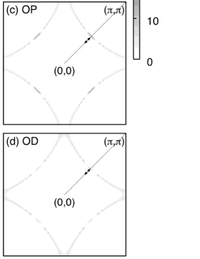
Figure 1: Fermi surfaces for ${}^{16}{\mathrm{O}}$ materials indicated in Table 1.

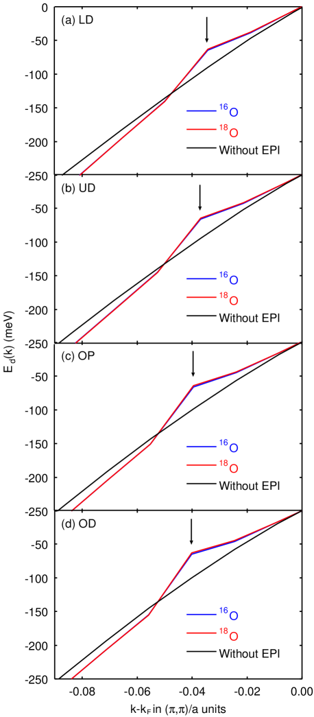
Figure 2: Dispersion kinks along the nodal direction. Momentum is measured from each Fermi surface. Arrows indicate the momenta at which kinks occur.

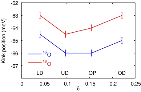
Figure 3: Doping dependence of kink energies. Bars indicate the discretization error during analytic continuation.

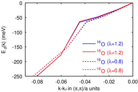
Figure 4: Dispersion kinks along the nodal direction for $\lambda=1.2$. The number of doped holes for ${}^{16}{\mathrm{O}}(^{18}{\mathrm{O}})$ material is $\delta=0.1309(0.1310)$. The dashed lines show the ones for OP in Table 1.

Figure 5: Dispersion kinks along the nodal direction for $\Delta_{dp}=1.8\,{\mathrm{eV}}$. The number of doped holes for ${}^{16}{\mathrm{O}}(^{18}{\mathrm{O}})$ material is $\delta=0.1621(0.1622)$. The dashed lines show the ones for OP in Table 1.

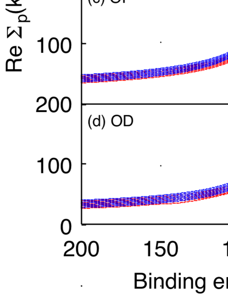
Figure 6: $\Sigma_{p}(\mathbf{k},\omega)$ on ${\mathbf{k}}=\left(\tilde{k}_{\mathrm{F}}-\frac{n}{64}\right)\!(\pi,\pi)\hskip 5.0pt(n=0,1,\ldots,5)$, where $\tilde{k}_{\mathrm{F}}=\frac{59}{128}$ for (a), $\tilde{k}_{\mathrm{F}}=\frac{57}{128}$ for (b), $\tilde{k}_{\mathrm{F}}=\frac{55}{128}$ for (c), and $\tilde{k}_{\mathrm{F}}=\frac{53}{128}$ for (d), respectively.

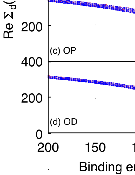
Figure 7: $\Sigma_{d}(\mathbf{k},\omega)$ on the same ${\mathbf{k}}$ points as in Fig. 4.

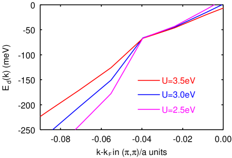
Figure 8: Dispersion kinks along the nodal direction for $U=2.5,3.0,$ and $3.5\,{\mathrm{eV}}$. They all correspond to OP. Momentum is measured from the Fermi surface for $U=3.0\,{\mathrm{eV}}$.

We show the numbers of doped holes for our fully self-consistent solutions in Table 1. The numbers of doped holes both for ${}^{16}{\mathrm{O}}$ and ${}^{18}{\mathrm{O}}$ materials are exactly the same to three places of decimals and they correspond to four different hole-doped samples, lightly doped (LD), underdoped (UD), optimally doped (OP), and overdoped (OD), respectively. In Fig. 1, we show the color map of the one-particle spectrum at Fermi level $A({\mathbf{k}},0)$, where

$$A({\mathbf{k}},\varepsilon)\equiv-\frac{1}{\pi}{\mathrm{Im}}\left\{{\mathrm{Tr\,}}\mathbf{G}(\mathbf{k},\mathrm{i}\epsilon_{n})\right\}_{\,\mathrm{i}\epsilon_{n}\rightarrow\varepsilon},$$ (20)

in order to indicate the Fermi surfaces for ${}^{16}{\mathrm{O}}$ materials. In Eq. (20), the Pad$\acute{\mathrm{e}}$ approximation is exploited for analytic continuation. Furthermore, we calculate the electronic dispersions of the antibonding band $E_{d}({\mathbf{k}})$ along the nodal direction indicated as the cut in Fig. 1 for all our doping cases. $E_{d}({\mathbf{k}})$ is determined as the $\mathbf{k}$ point on which $A({\mathbf{k}},\varepsilon)$ has the maximum value at each energy level. Due to this method, the curves of $E_{d}({\mathbf{k}})$ look like a series of line segments, as shown in Fig. 2. We compare every $E_{d}({\mathbf{k}})$ of our solution with the one obtained by another fully self-consistent manner, in which the same calculation is performed, except for the EPI. We show our results on these dispersions in Fig. 2, where we can easily recognize that the dispersion kinks along the nodal direction appear only when EPI affects the $p^{x(y)}$ electrons. The kink energies were slightly shifted by ${}^{16}{\mathrm{O}}\,\rightarrow\,^{18}{\mathrm{O}}$ substitution. In Fig. 3, we detail how these kink energies shift depending on hole doping. These theoretically evaluated isotope shifts are at most $2.5\,{\mathrm{meV}}$, which are much smaller than the ones measured by another group’s ARPES experiment. Gweon04 ; Gweon06 Furthermore, these isotope shifts are almost independent of hole doping while another group insists that they are critically affected. Gweon07 Considering the energy and momentum resolutions in their experiment, it may be hard to detect the subtle isotope shifts and their dependence on hole doping shown in our model.

Let us now look at $\lambda$ and $\Delta_{dp}$ dependences in the dispersion kinks along the nodal direction in detail. Figure 4 shows the energy dispersions for $\lambda=0.8$ (dotted lines) and $\lambda=1.2$ (solid lines). There is no clear difference in the isotope effect between $\lambda=1.2$ ($2.5\,{\mathrm{meV}}$) and $\lambda=0.8$ ($2.0\,{\mathrm{meV}}$), though the dispersion kinks for $\lambda=1.2$ are distinctly shifted to the high binding energy compared with those for $\lambda=0.8$. On the other hand, the isotope shift for $\Delta_{dp}=1.8\,{\mathrm{eV}}$ ($1\,{\mathrm{meV}}$) is slightly shrank compared to that for $\Delta_{dp}=1.4\,{\mathrm{eV}}$ ($2.5\,{\mathrm{meV}}$), though the dispersions depend on the $\Delta_{dp}$ considerably, as shown in Fig. 5. Hence, our model calculation shows that the isotope shifts are not sensitive to $\lambda$ and $\Delta_{dp}$. Considering that $\Delta_{dp}$ is closely related with EEI in our three band HH model as discussed later, we can be fairly certain that the isotope shifts are determined by the relative strength between EPI and EEI. However, these changes of the isotope shifts are minute, thus, our discussions so far are valid regardless of $\lambda$ and $\Delta_{dp}$.

To clarify the EPI effect on the $p^{x(y)}$ electrons described above, we investigate the $p$ electron self-energy $\Sigma_{p}(\mathbf{k},\omega)\equiv\Sigma_{x}(\mathbf{k},\omega)+\Sigma_{y}(\mathbf{k},\omega)$ along the nodal direction. In Fig. 6, we show $\Sigma_{p}(\mathbf{k},\omega)$ on every six $\mathbf{k}$ points along the nodal direction, located inside Fermi surfaces. The energy where $\Sigma_{p}(\mathbf{k},\omega)$ is maximal corresponds to the one of the dispersion kink and shifts upward by ${}^{16}{\mathrm{O}}\,\rightarrow\,^{18}{\mathrm{O}}$ substitution, as shown in Fig. 2. The energy dependence of $\Sigma_{p}(\mathbf{k},\omega)$ is definitely due to the EPI introduced with the use of Eqs. (14), (18), and (19). Thus, we can conclude that in our solutions for all doping levels from the UD to the OD region, the dispersion kinks along the nodal direction are created only when the EPI is included.

Hereafter, we will discuss why the magnetic ingredients hardly bring the dispersion kinks along the nodal direction. Even when EPI does not exist, the electrons in our results are exposed to the strong AF fluctuation originating from the electronic correlation among $d$ electrons. In Fig. 7, we show $\Sigma_{d}(\mathbf{k},\omega)$ on the same six $\mathbf{k}$ points as in Fig. 6. It is shown that there is no clear difference in $\Sigma_{d}(\mathbf{k},\omega)$ between ${}^{16}{\mathrm{O}}$ and ${}^{18}{\mathrm{O}}$ materials. The energy dependence of $\Sigma_{d}(\mathbf{k},\omega)$ is definitely due to the electronic correlation introduced with the use of Eqs. (15)–(17). We easily recognize that $\Sigma_{d}(\mathbf{k},\omega)$ uniformly increases with the binding energy and has no maximal value up to $200\,{\mathrm{meV}}$ even for LD case, in which the strong AF fluctuation is expected to be grown. Thus, along the nodal direction, the strong AF fluctuation could cause the renormalization of the Fermi velocity, however, it hardly promotes any anomalous behavior such as kink structure.

Finally, we will discuss how our EEI affects the dispersion for ${}^{16}{\mathrm{O}}$ materials. When the on-site Coulomb repulsion $U$ is changed, the Fermi velocity is renormalized differently, but this would not change the kink energy so much since the kink energy is determined by the EPI alone. In Fig. 8, we lay out our results for three different $U$s and they all correspond to OP. Their total doped holes $\delta$ are slightly different as: $\delta=0.158,0.154,$ and $0.149$ for $U=2.5,3.0,$ and $3.5\,{\mathrm{eV}}$, respectively. Hence, the Fermi momentum for $U=2.5\,{\mathrm{eV}}$ moves inside (or the Fermi surface shrinks) and the one for $U=3.5\,{\mathrm{eV}}$ moves outside (or the Fermi surface enlarges), compared to the one for $U=3.0\,{\mathrm{eV}}$. These changes of the Fermi momenta are small; however, the dispersions at higher energy are quite affected, reflecting the binding energy dependence of $\Sigma_{d}(\mathbf{k},\omega)$, as shown in Fig. 7. Therefore, the dispersion at higher energy could be changed a lot by the EEI even if the Fermi velocities are almost independent of them.

CONCLUSIONS

By the analysis of our model, we can show that the dispersion kink along the nodal direction occurs due to EPI. The isotope effect upon the electronic dispersion is shown near the kink of energy dispersion, not in the high binding energy portions.  Gweon04 ; Gweon06 Our evaluation of the subtle isotope shifts has been backed by the report of the recent ARPES experiments Douglas07 ; Iwasawa07 which show the lack of the unusual isotope effect in the high energy portion. Gweon04 ; Gweon06 ; Gweon07 Fortunately for us, our scenario was possibly realized in further ARPES experiment. Iwasawa08 In addition to that, we have investigated how EEI effects on the nodal dispersion. It can hardly affect the kink and the nodal Fermi velocity; however, it can change the dispersion at higher energy. Hence, EPI and EEI play different roles on the nodal energy dispersion, respectively.

Of course, our treatment of EEI is just suited for weak coupling regime, and all of our parameter sets employed might be far from the ones for strong coupling regime. If we investigate strong coupling regime with the use of another approach, the low energy structure corresponding to the superexchange $J$ could appear in the dispersion. However, our results presented here suggest that the structure should appear as a broad peak at higher energy due to the frequency dependence of the strong AF fluctuation, which will grow into $J$. As we all know, other works have already derive qualitatively similar conclusions on the basis of other models. Some groups adopt $t$-$J$ models  Rosch04 ; Ishihara04 ; Mishchenko04 ; Mishchenko06 and other groups do one-band HH models. Fratini05 ; Sangiovanni06 ; Paci06 Furthermore, other groups have succeeded in explaining the ARPES results. Cuk04 ; Devereaux04 ; Seibold05 ; Maksimov05 ; Meevasana06 ; Heid07 However, in our 2D three-band HH model, both the electron-electron interaction among the $d$ electrons and the EPI on $p$ electrons are considered according to high-$T_{\mathrm{c}}$ materials. We believe that it is important that quantitatively consistent results with the ARPES experiments can be reproduced from such a model. The advantage will be when our analysis extends to the superconducting state, in which the $p$ electrons play important roles as well as $d$ electrons.

References

- (1) A. Kaminski, M. Randeria, J. C. Campuzano, M. R. Norman, H. Fretwell, J. Mesot, T. Sato, T. Takahashi, and K. Kadowaki, Phys. Rev. Lett. 86, 1070 (2001).
- (2) A. Lanzara, P. V. Bogdanov, X. J. Zhou, S. A. Kellar, D. L. Feng, E. D. Lu, T. Yoshida, H. Eisaki, A. Fujimori, K. Kishio, J.-I. Shimoyama, T. Noda, S. Uchida, Z. Hussain, and Z.-X. Shen, Nature (London) 412, 510 (2001).
- (3) X. J. Zhou, T. Yoshida, A. Lanzara, P. V. Bogdanov, S. A. Kellar, K. M. Shen, W. L. Yang, E. Ronning, T. Sasagawa, T. Kakeshita, T. Noda, H. Eisaki, S. Uchida, C. T. Lin, F. Zhou, J. W. Xiong, W. X. Ti, Z. X. Zhao, A. Fujimori, Z. Hussain, and Z.-X. Shen, Nature (London) 423, 398 (2003).
- (4) Z.-X. Shen, A. Lanzara, S. Ishihara, and N. Nagaosa, Philos. Mag. 82, 1394 (2002).
- (5) K. Terashima, H. Matsui, D. Hashimoto, T. Sato, T. Takahashi, H. Ding, T.Yamamoto, and K. Kadowaki, Nat. Phys. 2, 27 (2006).
- (6) V. B. Zabolotnyy, S. V. Borisenko, A. A. Kordyuk, J. Fink, J. Geck, A. Koitzsch, M. Knupfer, B. Büchner, H. Berger, A. Erb, C. T. Lin, B. Keimer, and R. Follath, Phys. Rev. Lett. 96, 037003 (2006).
- (7) A. A. Kordyuk, S. V. Borisenko, V. B. Zabolotnyy, J. Geck, M. Knupfer, J. Fink, B. Büchner, C. T. Lin, B. Keimer, H. Berger, A. V. Pan, S. Komiya, and Y. Ando, Phys. Rev. Lett. 97, 017002 (2006).
- (8) J. Lee, K. Fujita, K. McElroy, J. A. Slezak, M. Wang, Y. Aiura, H. Bando, M. Ishikado, T. Matsui, J.-X. Zhu, A. V. Balatsky, H. Eisaki, S. Uchida, and J. C. Davis, Nature (London) 442, 546 (2006).
- (9) R. J. McQueeney, J. L. Sarrao, P. G. Pagliuso, P. W. Stephens, and R. Osborn, Phys. Rev. Lett. 87, 077001 (2001).
- (10) N. E. Bickers and D. J. Scalapino, Ann. Phys. (N.Y.) 193, 206 (1989).
- (11) D. L. Feng, N. P. Armitage, D. H. Lu, A. Damascelli, J. P. Hu, P. Bogdanov, A. Lanzara, F. Ronning, K. M. Shen, H. Eisaki, C. Kim, J.-i. Shimoyama, K. Kishio, and Z.-X. Shen, Phys. Rev. Lett. 86, 5550 (2001).
- (12) Y.-D. Chuang, A. D. Gromko, A. Fedorov, Y. Aiura, K. Oka, Yoichi Ando, H. Eisaki, S. I. Uchida, and D. S. Dessau, Phys. Rev. Lett. 87, 117002 (2001).
- (13) G.-H. Gweon, T. Sasagawa, S. Y. Zhou, J. Graf, H. Takagi, D.-H. Lee, and A. Lanzara, Nature (London) 430, 187 (2004).
- (14) G.-H. Gweon, S. Y. Zhou, M. C. Watson, T. Sasagawa, H. Takagi, and A. Lanzara, Phys. Rev. Lett. 97, 227001 (2006).
- (15) G.-H. Gweon, T. Sasagawa, H. Takagi, D.-H. Lee, and A. Lanzara, arXiv:0708.1027.
- (16) J. F. Douglas, H. Iwasawa, Z. Sun, A. V. Fedorov, M. Ishikado, T. Saitoh, H. Eisaki, H. Bando, T. Iwase, A. Ino, M. Arita, K. Shimada, H. Namatame, M. Taniguchi, T. Masui, S. Tajima, K. Fujita, S. Uchida, Y. Aiura, and D. S. Dessau, Nature (London) 446, E5 (2007).
- (17) H. Iwasawa, Y. Aiura, T. Saitoh, H. Eisaki, H. Bando, A. Ino, M. Arita, K. Shimada, H. Namatame, M. Taniguchi, T. Masui, S. Tajima, M. Ishikado, K. Fujita, S. Uchida, J. F. Douglas, Z. Sun, and D. S. Dessau, Physica C 463-465, 52 (2007).
- (18) H. Iwasawa, J. F. Douglas, K. Sato, T. Masui, Y. Yoshida, Z. Sun, H. Eisaki, H. Bando, A. Ino, M. Arita, K. Shimada, H. Namatame, M. Taniguchi, S. Tajima, S. Uchida, T. Saitoh, D. S. Dessau, and Y. Aiura (unpublished).
- (19) O. Rsch and O. Gunnarsson, Phys. Rev. Lett. 92, 146403 (2004).
- (20) S. Ishihara and N. Nagaosa, Phys. Rev. B 69, 144520 (2004).
- (21) A. S. Mishchenko and N. Nagaosa, Phys. Rev. Lett 93, 036402 (2004).
- (22) A. S. Mishchenko and N. Nagaosa, Phys. Rev. B 73, 092502 (2006).
- (23) S. Fratini and S. Ciuchi, Phys. Rev. B 72, 235107 (2005).
- (24) G. Sangiovanni, O. Gunnarsson, E. Koch, C. Castellani, and M. Capone, Phys. Rev. Lett. 97, 046404 (2006).
- (25) P. Paci, M. Capone, E. Cappelluti, S. Ciuchi, and C. Grimaldi, Phys. Rev. B. 74, 205108 (2006).
- (26) T. Cuk, F. Baumberger, D. H. Lu, N. Ingle, X. J. Zhou, H. Eisaki, N. Kaneko, Z. Hussain, T. P. Devereaux, N. Nagaosa, and Z.-X. Shen, Phys. Rev. Lett. 93, 117003 (2004).
- (27) T. P. Devereaux, T. Cuk, Z. X. Shen, and N. Nagaosa, Phys. Rev. Lett. 93, 117004 (2004).
- (28) G. Seibold and M. Grilli, Phys. Rev. B 72, 104519 (2005).
- (29) E. G. Maksimov, O. V. Dolgov, and M. L. Kulic, Phys. Rev. B 72, 212505 (2005).
- (30) W. Meevasana, N. J. C. Ingle, D. H. Lu, J. R. Shi, F. Baumberger, K. M. Shen, W. S. Lee, T. Cuk, H. Eisaki, T. P. Devereaux, N. Nagaosa, J. Zaanen, and Z.-X. Shen, Phys. Rev. Lett. 96, 157003 (2006).
- (31) R. Heid, K.-P. Bohnen, R. Zeyher, and D. Manske, Phys. Rev. Lett. 100, 137001 (2008).