Anatomy of luminosity functions: the 2dFGRS example

Abstract

Aims. We use the 2dF Galaxy Redshift Survey to derive the luminosity function (LF) of the first-ranked (brightest) group/cluster galaxies, the LF of second-ranked, satellite and isolated galaxies, and the LF of groups of galaxies.

Methods. We investigate the LFs of different samples in various environments: in voids, filaments, superclusters and supercluster cores. We compare the derived LFs with the Schechter and double-power-law analytical expressions. We also analyze the luminosities of isolated galaxies.

Results. We find strong environmental dependency of luminosity functions of all populations. The luminosities of first-ranked galaxies have a lower limit, depending on the global environment (higher in supercluster cores, and absent in voids). The LF of second-ranked galaxies in high-density regions is similar to the LF of first-ranked galaxies in a lower-density environment. The brightest isolated galaxies can be identified with first-ranked galaxies at distances where the remaining galaxies lie outside the observational window used in the survey.

Conclusions. The galaxy and cluster LFs can be well approximated by a double-power-law; the widely used Schechter function does not describe well the bright end and the bend of the LFs. Properties of the LFs reflect differences in the evolution of galaxies and their groups in different environments.

1 Introduction

Groups and clusters of galaxies are the most common environment of galaxies. In particular, groups of galaxies are locations of galaxy formation, and their study yields information on the processes of galaxy formation and evolution. Clusters of galaxies form basically by hierarchical merging of smaller units – galaxies and groups of galaxies. In groups and clusters the evolution of galaxies differs from that in low-density regions.

The presence of satellite galaxies around our Galaxy and the Andromeda galaxy is known long ago. Systematic studies of physical groups of galaxies were pioneered by Holmberg (1969); de Vaucouleurs & de Vaucouleurs (1970); Turner & Sargent (1974), followed by Geller & Huchra (1983); Nolthenius & White (1987); Tully (1987); Maia et al. (1989); Ramella et al. (1989); Gourgoulhon et al. (1992); Garcia (1993); Moore et al. (1993), and many others. First large catalogues of clusters of galaxies were constructed by visual inspection of the Palomar Observatory Sky Survey plates by Abell (1958); Zwicky & Kowal (1968); Abell et al. (1989). More recently clusters of galaxies were selected also using their X-ray emission by Gioia et al. (1990); Ebeling et al. (1996); Böhringer et al. (2001). Deeper redshift surveys made it possible to construct group and cluster catalogues for more distant objects: e.g., the Las Campanas Redshift Survey was used by Tucker et al. (2000) to construct a catalogue of loose groups. The ’100k’ public release of the 2 degree Field Galaxy Redshift Survey (2dFGRS), described by Colless et al. (2003), has been used to construct several catalogues of groups. Among them, there are the catalogues by Merchán & Zandivarez (2002), by Yang et al. (2005a), and by Tago et al. (2006, hereafter T06). Eke et al. (2004a) used the complete 2dFGRS to compile a sample of about 25 thousand groups and clusters in the two contiguous Northern and Southern Galactic Patches.

One of the principal description functions for clusters and groups of galaxies is the luminosity function $F(L)$ that describes the average number of galaxies per unit volume as a function of galaxy luminosity. The luminosity function (LF) plays an important role in our understanding how galaxies form and evolve (van den Bosch et al. 2003; Yang et al. 2003; Cooray & Cen 2005; Cooray & Milosavljević 2005a; Cooray 2006; Milosavljević et al. 2006; Tinker et al. 2005, 2007; Hansen et al. 2007; van den Bosch et al. 2007; Tinker & Conroy 2008).

The LF of groups of galaxies was first derived by Holmberg (1969), followed by Christensen (1975); Kiang (1976); Abell (1977); Mottmann & Abell (1977). These studies showed that the LF of galaxies in groups and clusters can be approximated by a double-power-law, the crossover between two powers occurs at a characteristic absolute magnitude $M^{*}\approx-20-5\log h$.

Our interest in the structure of groups of galaxies began with the discovery of dark matter coronas (haloes) around giant galaxies (Einasto et al. 1974a). We noticed that practically all giant galaxies are surrounded by dwarf companion galaxies, and that such systems have a certain structure: elliptical companions are concentrated near the dominating (brightest) galaxy, and spiral and irregular companions lie at the periphery of the system (Einasto et al. 1974b). The LF of these systems has a specific feature: the luminosity of the brightest galaxy of the system exceeds the luminosity of all companion galaxies by a large factor, thus the overall relative LF of the system – the conditional luminosity function – has a gap separating the brightest galaxy from companion galaxies (Einasto et al. 1974c). Dynamically these systems are dominated by dark matter, and there exist clear signatures of mutual interactions between galaxies and intergalactic matter in these systems, as shown by Einasto et al. (1974b, 1975); Chernin et al. (1976); Einasto et al. (1976) (for a review of dark matter around galaxies see Faber & Gallagher (1979)). The morphology-density relation in clusters was investigated by Oemler (1974); Dressler (1980); Postman & Geller (1984). We see that it is valid also in ordinary groups. In other words, groups of galaxies are not just random collections of galaxies, they form systems with various mutual interactions. The whole system of companion galaxies lies inside the dark corona (halo) of the brightest galaxy and can be considered as one physical entity. To stress this aspect we called such systems hypergalaxies (Einasto et al. 1974c). Our first catalogue of hypergalaxies (groups with a dominating brightest galaxy) was composed by Einasto et al. (1977). In recent years the study of the connection between dark matter haloes and galaxies has made great progress, in particular using the halo occupation distribution model; for details see, among others, Kauffmann et al. (1997); Tinker et al. (2005); Yang et al. (2005a); Zehavi et al. (2005); Tinker et al. (2006); Zheng et al. (2007); Yang et al. (2008b).

The dominating role of the brightest (first-ranked) cluster/group galaxies was known long ago, for early studies see Hubble & Humason (1931); Hubble (1936); Sandage (1976). The nature of physical processes which influence the luminosity and morphology of galaxies in clusters (and groups) is also known: tidal-stripping of gas during close encounters and mergers (Spitzer & Baade 1951), ram-pressure sweeping of gas due to galaxy motion through the intra-cluster medium (Gunn & Gott III 1972; Chernin et al. 1976; van den Bosch et al. 2008), galaxy mergers (Toomre & Toomre 1972).

To understand details of these processes it is important to study properties of galaxies in groups and clusters. Indeed, in last years the number of studies devoted to the study of LFs in groups and clusters has increased. We note here the work by Ferguson & Sandage (1988, 1991); van den Bergh (1992); Moore et al. (1993); Sulentic & Rabaca (1994); Ribeiro et al. (1994); Zepf et al. (1997); Hunsberger et al. (1998); Muriel et al. (1998); Zabludoff & Mulchaey (2000); Popesso et al. (2005); Miles et al. (2004, 2006); González et al. (2005, 2006); Berlind et al. (2006); Chiboucas & Mateo (2006); Lin et al. (2006); Zandivarez et al. (2006); Adami et al. (2007); Hansen et al. (2007); Milne et al. (2007); Vale & Ostriker (2006, 2008).

The present analysis has three goals: to determine the LF of group brightest (first-ranked), second-ranked and satellite galaxies; to investigate the nature of satellite and isolated galaxies; and to analyze environmental dependency of galaxy luminosities. As there are no strict differences between groups and clusters of galaxies we shall use the term “group” for groups of galaxies as well as for conventional clusters. To derive the LFs we shall use the catalogue of groups and clusters by Tago et al. (T06). This catalogue was prepared using the 2dFGRS Northern and Southern Galactic Patches, similar catalogues have been compiled by Eke et al. (2004a); Yang et al. (2005a) and several other authors. As in all such catalogues, we find a number of isolated galaxies, i.e. galaxies which have no neighbours within the search radius in the flux-limited galaxy survey. We analyse the luminosity distribution of isolated galaxies and show that a large fraction of these galaxies can be considered as brightest galaxies of groups where fainter members of the group lie outside the visibility window of the survey. As a by-product we derive also the LF of groups.

LFs of simulated groups and groups found for the 2dFGRS and the Sloan Digital Sky Survey Data Release 4 have been recently studied, among others, by Mo et al. (2004); Yang et al. (2004); Cooray & Cen (2005); Cooray & Milosavljević (2005a); Croton et al. (2005); Zheng et al. (2005); Tinker & Conroy (2008); Yang et al. (2008a). In many of these papers the emphasis has been on explanation of the LF using halo occupation statistics. Our motivation in this paper is mostly observational; we shall study the connection of the observed LF with sub-halo model data in a separate paper (in preparation). Here we shall discuss the nature of second-ranked and satellite galaxies in more detail, and shall search for the dependence of the LFs of the brightest and satellite galaxies on the environment.

The observational data are discussed in the next Section; here we consider also the selection effects and the methods to correct data for selection. In Sect. 3 we calculate the LFs of group brightest, second-ranked, satellite and isolated galaxies. We derive the LFs for different environmental densities. The nature of isolated galaxies is discussed in Sect. 4. The LFs of various galaxy samples and the LF of groups are derived in Sect. 5: here we compare the Schechter and double-power-law expressions. We discuss our results and bring conclusions in Sects. 6 and 7, respectively.

Table 1: Data on the 2dFGRS galaxies and groups used

Sample	$\Delta$RA	$\Delta$DEC	$N_{\rm gal}$	$N_{\rm gr}$	$N_{\rm isol}$
	deg	deg
1	2	3	4	5	6
NGP	$75^{\circ}$	$10^{\circ}$	78067	10750	44134
SGP	$90^{\circ}$	$13.5^{\circ}$	106328	14465	61344

Columns:

• the subsample of the 2dFGRS catalogue.

• sample width in right ascension (degrees).

• sample width in declination (degrees).

• total number of galaxies.

• number of groups.

• number of isolated galaxies.

Figure 1: Luminosities of first-ranked galaxies in the 2dFGRS at various distances from the observer.

2 Data

2.1 The group catalogue

In the present analysis we shall use the catalogue of groups and clusters by Tago et al. (T06). This catalogue covers the contiguous 2dFGRS Northern and Southern Galactic Patches (NGP and SGP, respectively), small fields spread over the southern Galactic cap are excluded. We extracted data on galaxies from the 2dFGRS web-site (http://www.mso.anu.edu.au/2dFGRS): the coordinates RA and DEC, the apparent magnitudes in the photometric system $b_{J}$, the redshifts $z$, and the spectral energy distribution parameters $\eta$. We excluded distant galaxies with redshifts $z>0.2$, since weights to calculate expected total luminosities (see Sect. 5.2) become too large and uncertain at these redshifts. The apparent magnitude interval of the 2dFGRS ranges from $m_{1}=14.0$ to the survey faint limit $m_{2}\approx 19.45$ (in the photometric system $b_{J}$, corrected for the Galactic extinction). Actually the faint limit $m_{2}$ varies from field to field. In calculation of the luminosity weights these deviations have been taken into account, as well as the incompleteness of the survey (the fraction of observed galaxies among all galaxies up to the fixed magnitude limit; for details see T06). The number of galaxies selected for the analysis is given in Table 1. For linear dimensions we use co-moving distances (see, e.g. Martínez & Saar 2003), computed using a $\Lambda$CDM cosmological model with the following parameters: the matter density $\Omega_{\mathrm{m}}=0.3$, and the dark energy density $\Omega_{\Lambda}=0.7$.

In the group definition T06 tried to avoid the inclusion of large sections of underlying filaments or surrounding regions of superclusters into groups. To find the appropriate search radius (FoF radius) for group definition T06 investigated the behaviour of roups, if artificially shifted to larger distances from the observer. Using this method T06 found that the search radius to find group members must increase with distance only moderately.

To transform the apparent magnitude $m_{J}$ into the absolute magnitude $M$ we use the usual formula

$$M=m_{J}-25-5\log_{10}(d_{L})-K,$$ (1)

where the luminosity distance is $d_{L}=d(1+z)$, $d$ is the co-moving distance in the units of $h^{-1}$ Mpc, and $z$ is the observed redshift. The term $K$ is the $k\!+\!e$-correction, adopted according to Norberg et al. (2002).

2.2 Selection effects: visibility of galaxies at different distances

To calculate the LF of galaxies we need to know the number of galaxies of a given luminosity per unit volume. The principal selection effect in flux-limited surveys is the absence of galaxies fainter than the survey limiting magnitude. This effect is well seen in Fig. 1 that shows the luminosities of the first-ranked galaxies at various distances from the observer.

To take this effect into account in the determination of the LF of group galaxies we used the standard $V_{\mathrm{max}}^{-1}$ weighting procedure. The differential luminosity function $n(L)$ (the expectation of the number density of galaxies of the luminosity $L$) can be found as follows:

$$n(L){\mathrm{d}}L=\sum_{i}\frac{\mathbf{I}_{(L,L+\mathrm{d}L)}(L_{i})}{V_{\mathrm{max}}(L_{i})},$$ (2)

where $\mathrm{d}L$ is the luminosity bin width, $\mathbf{I}_{A}(x)$ is the indicator function that selects the galaxies that belong to a particular luminosity bin, $V_{\mathrm{max}}(L)$ is the maximum volume where a galaxy of a luminosity $L$ can be observed in the present survey, and the sum is over all galaxies of the survey. This procedure is non-parametric, and gives both the form and true normalization of the LF.

We select galaxies in the distance interval 70–500 $h^{-1}$ Mpc. At small distances, bright galaxies are absent from the survey (see Fig. 1) due to the limiting bright apparent magnitude of the survey. To avoid this selection effect, we set the lower distance limit to 70 $h^{-1}$ Mpc. The upper limit is set to 500 $h^{-1}$ Mpc since at large distances the weights for restoring group luminosities become too big (see Fig. 14).

2.3 Determination of environmental densities

Already early studies of the distribution of galaxies of different luminosity showed that clustering of galaxies depends on their luminosity (Hamilton 1988; Einasto 1991), and thus the LF of galaxies depends on the environment where the galaxy is located (Cuesta-Bolao & Serna 2003; Mo et al. 2004; Croton et al. 2005; Hoyle et al. 2005; Xia et al. 2006). Recent studies have demonstrated that both the local (group) as well as the global (supercluster) environments play a role in determining properties of galaxies, including their luminosities (Einasto et al. 2007b). To estimate these effects and to investigate the dependence of the galaxy LF on the environment we calculated the luminosity density field.

Table 2: The numbers of first-ranked, satellite and isolated galaxies in different environments

Population	D1	D2	D3	D4
	Void	Filament	Supercluster	SC Core
	$D\!\leq 1.5$	$1.5<\!D\!\leq 4.6$	$4.6<\!D\!\leq 7$	$D\!>7$
First-ranked	5499	11979	3511	2261
Satellites	8196	24078	9561	8582
Isolated gal.	36813	40553	8263	4359

• The density parameter $D$ is the global environmental density in units of the mean density (see Sect. 2.3 for more information).

To calculate the density field we need to know the expected total luminosities of groups and isolated galaxies (a detailed description of calculating these luminosities is given in Sect. 5.2). These quantities are given in the group catalogue by T06. The luminosity density fields were found using kernel smoothing as described in our 2dFGRS supercluster catalogue (Einasto et al. 2007a):

$$D(\mathbf{x})=\sum_{i}K(\mathbf{x-x}_{i};h)\,L_{i},$$ (3)

where $K(\mathbf{x};h)$ is a suitable kernel of a width $h$ with a unit volume integral, and $L_{i}$ is the luminosity of the $i$-th galaxy. The sum extends formally over all galaxies, but the kernel is usually chosen to differ from zero only in a limited range of the argument; this limits the number of galaxies in the sum. For details see Einasto et al. (2007a).

We used the Epanechnikov kernel:

$$K_{\mathrm{E}}(\mathbf{x};h)=\frac{15}{8\pi h^{3}}(1-\mathbf{x}^{2}/h^{2})\;,\quad\mathbf{x}^{2}\leq h^{2},\;\quad 0\quad\mathrm{otherwise},$$ (4)

of a radius $h=8\,$$h^{-1}$ Mpc.

After that, we divided all groups (galaxies) into classes, according to the value of the global environmental density $D$ at their location as follows: low density regions with $D\leq 1.5$, medium density regions with $1.5<D\leq 4.6$, high density regions with $4.6<D\leq 7$, and very high density regions with $D>7$ (all densities are in units of the mean luminosity density for the sample volume); we denote these regions as D1, D2, D3, D4, respectively. The threshold density 4.6 was used in our supercluster catalogue (Einasto et al. 2007a) to separate superclusters from field objects. We define superclusters as non-percolating high-density regions of the cosmic web using the global density to discriminate between objects belonging to superclusters or to the field (see Fig. 16 below for illustration). Einasto et al. (2007b) showed that the densities $D>7$ are characteristic to supercluster cores. High density cores are present in rich superclusters only. The supercluster environment represents poor superclusters and the outskirt regions of rich superclusters. As seen from Fig. 16, supercluster cores may have a complex internal structure, consisting of clusters and groups and even isolated galaxies. The threshold density 1.5 that separates the low and medium density regions corresponds approximately to the division between galaxies in voids and those in filaments. These divisions are not directly related to the shape or other properties of galaxy systems (for a recent discussion of the properties of DM haloes in different environments see Hahn et al. (2007)).

We use these four density classes to study the environmental dependences of the LFs. In Table 2 we show the number of galaxies in different environments for different populations (first-ranked galaxies, group satellite galaxies and isolated galaxies). Everywhere in this paper the supercluster class usually does not include galaxies in supercluster cores; if we lump these classes together, we tell that.

3 Luminosity functions in different environments

3.1 Brightest group galaxies

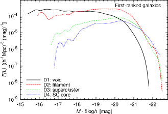
Figure 2: The differential LFs of first-ranked galaxies. The functions have been calculated for four classes of global environmental density: D1, D2, D3, D4 (voids, filaments, superclusters, cores of superclusters), with limiting densities 1.5, 4.6 and 7 in units of the mean density. Solid line – void galaxies; dashed line – filament galaxies; short dashed line – supercluster galaxies; dotted line – supercluster core galaxies.

We use our galaxy samples and the catalogue of groups of galaxies (T06) to calculate the LF for first-ranked (brightest group) galaxies. The catalogue by T06 gives for each group the luminosity of the first-ranked galaxy (most luminous in the $b_{J}$-filter). In the present study we shall made no effort to use for the first-ranked galaxy identification other galaxy properties, such as spectral type, colour index or possible activity. These morphological aspects deserve a more detailed study which is outside the scope of the present investigation.

We calculated the differential LF of first-ranked galaxies in various environments for different samples. The numbers of galaxies used are given in Table 2.

The differential LFs of first-ranked galaxies are shown in Fig. 2 for different environmental densities. In order not to overcrowd the figures, we do not show error bars. As there are many galaxies, errors are small; typical errors are illustrated in Fig. 4.

Figure 2 shows that there exist large differences between LFs in different environmental regions. The brightest first-ranked galaxies in void regions have a factor of 3–4 lower luminosity than the brightest first-ranked galaxies in regions of higher environmental densities. For this reason the whole LF of void first-ranked galaxies is shifted toward lower luminosities. At the same time, there are no significant differences between the luminosities of the brightest first-ranked galaxies in the filament, supercluster, and supercluster core environments. Later we shall see that the same is valid for satellite galaxies.

The second large difference between the first-ranked galaxy luminosities in various environments is the presence of a well-defined lower limit of first-ranked galaxy luminosities in the superclusters and cores of superclusters. In supercluster cores the lower first-ranked galaxy luminosity limit is about $-17\,$mag. When we move to lower environmental densities, the lower first-ranked galaxy luminosity limit gets smaller (see Fig. 2). The supercluster core environment forces lower limits also for other galaxies (satellites and isolated galaxies). The void and filament first-ranked galaxies do not have any lower luminosity limit.

3.2 Group second-ranked galaxies

We define the group second-ranked galaxy as the most luminous satellite galaxy in the group: it is the second luminous galaxy in the group.

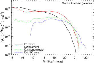
Figure 3: The differential LFs of group second-ranked galaxies. Labels are the same as in Fig. 2.

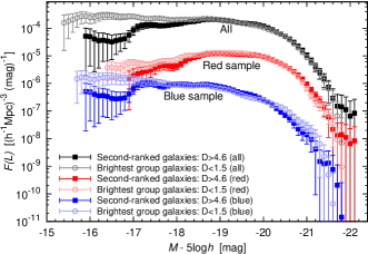
Figure 4: The differential LFs of two populations: filled squares – second-ranked galaxies in the supercluster (including the supercluster core) environment ($D>4.6$); open circles – first-ranked galaxies in the void environment ($D<1.5$). Upper (black) points are for all galaxies; middle (red) points are for the red population (shifted down by one unit in the $\log(F(L))$ scale); bottom (blue) points are for the blue population (shifted down by two units in the $\log(F(L))$ scale).

In Fig. 3 we plot the differential LFs of group second-ranked galaxies in different environments. The overall picture is similar to the LFs of first-ranked galaxies. The primary difference is that the bright end of the LF is shifted to lower luminosities. The faint-end limits are approximately the same as for first-ranked galaxies.

Another difference (compared with first-ranked galaxies) is that the brightest second-ranked galaxies in the supercluster core environment are more luminous than the brightest galaxies in the supercluster and filament environments; for first-ranked galaxies the bright end of the LFs was the same for these three environments.

This effect is expected if second-ranked galaxies in high density environments had been first-ranked galaxies before they were drawn into a larger cluster via merging of groups into larger systems. Thus the LF of second-ranked galaxies in high density regions is more close to the LF of first-ranked galaxies than to the LF of second-ranked galaxies in low density regions.

To test this last assumption, we plotted in Fig. 4 the differential LFs of two populations: the first population consists of the second-ranked galaxies in the supercluster environment (including the supercluster core environment); the second sample includes the first-ranked galaxies in the void region. The error-bars in this plot are Poisson 1-$\sigma$ errors; in other figures (where only lines are shown) the errors have the same order of magnitude. We see that these two distributions are pretty similar. There are differences at the faint end, but these are caused by the environment; there are only a few faint first- and second-ranked galaxies in high-density regions. Thus we see that the second-ranked galaxy LF in high-density regions is similar to the first-ranked galaxy LF in the low-density environment.

To show that this similiarity is not accidental, we divided these galaxies into two samples (red and blue galaxies), using information about the colours of galaxies (the rest-frame colour index, $col=(B-R)_{0}$, Cole et al. (2005)). We used the limit $col=1.07$ to separate the populations of red (passive) and blue (actively star-forming) galaxies. For these two samples the LFs are still similar (see Fig. 4), only the supercluster galaxies are in average 0.15 mag redder than the void galaxies. This shift was also seen in Einasto et al. (2007b) where we showed that not only the brightest galaxies, but all galaxies in superclusters are redder than those in voids.

The first-ranked galaxy population is different from that of the satellite galaxy population, but the changeover from one population to the other is smooth.

3.3 Other satellite galaxies

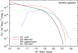
Figure 5: The differential LFs of satellite galaxies. Labels are the same as in Fig. 2.

Group satellite galaxies are all galaxies in groups (excluding first-ranked galaxies). The satellite galaxy population includes also the second-ranked galaxies.

In Fig. 5 we show differential LFs of group satellite galaxies. The LFs are similar to the LFs of second-ranked galaxies. The primary difference is that the faint satellites in the supercluster and supercluster core environments have lower luminosities, and there are more faint satellites than faint second-ranked galaxies. In supercluster cores, the brightest satellites are more luminous than those in lower density environments. In addition, in the highest density environment there exists a sharp lower satellite luminosity limit.

3.4 Isolated galaxies

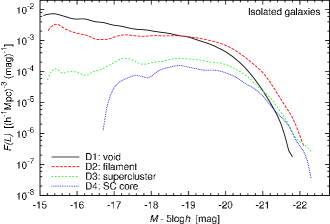
Figure 6: The differential LFs of isolated galaxies. Labels are the same as in Fig. 2.

We define all galaxies that do not belong to groups/clusters in the T06 group catalogue, as isolated galaxies. In this section we present the LFs of isolated galaxies; we shall discuss the nature of isolated galaxies later, in a separate section.

In Fig. 6 we show the differential LFs of isolated galaxies in different environments. Isolated galaxies in the supercluster core environment have a faint luminosity limit (similar to other populations). The differences in the LFs of bright isolated galaxies between various environments are much smaller than for other populations. The brightest isolated galaxies occur in the filament environment (for other populations the brightest galaxies can be found in the supercluster core environment). This means that in the supercluster and supercluster core environments the brightest galaxies lie in groups/clusters, contrary to the void and filament environments, where many bright galaxies are identified as isolated galaxies.

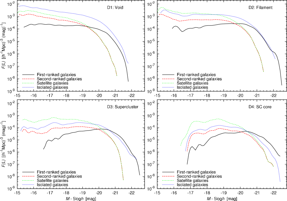
Figure 7: Differential LFs in different environments and for different galaxy populations. Top-left panel – void environment; top-right panel – filament environment; bottom-left panel – supercluster environment; bottom-right panel – supercluster core environment. Solid line shows first-ranked galaxies; dashed line – second-ranked galaxies; short-dashed line – satellite galaxies; dotted line – isolated galaxies.

3.5 Comparison of LFs in different environments

Differential LFs of galaxy populations in various environments are shown in Fig. 7. Each panel represents a different environment, and in each panel we show the LFs of different populations (first-ranked, second-ranked, satellite and isolated galaxies).

Figure 7 (upper-left panel) shows that in voids, the bright end of LFs of all galaxy populations is shifted toward lower luminosities – in the void environment first-ranked galaxies of groups are fainter than those in higher density environments. We noticed this effect also in Einasto et al. (2007b). Interestingly, the bright end of the LF for isolated galaxies in voids is comparable to that of first-ranked galaxies. We discuss the possible reasons for that in the next section. The LFs of second-ranked galaxies and of all satellites are comparable, although there is a slight increase of the LF of satellite galaxies at the lowest luminosities. The LF of first-ranked galaxies, in contrary, has a plateau at the faint end, without signs of increase.

In the filament environment (Fig. 7, upper-right panel) the bright ends of the LFs for first-ranked galaxies and for isolated galaxies are similar, while the brightest second-ranked galaxies and satellite galaxies are fainter. For a wide range of luminosities, the LF for first-ranked galaxies is slowly decreasing toward fainter luminosities, while LFs for other galaxy populations have a plateau.

The LFs for the supercluster environment (excluding supercluster cores) are shown in the lower-left panel of Fig. 7. As we mentioned, the supercluster environment represents poor superclusters and the outskirt regions of rich superclusters. This Figure shows that the first-ranked galaxies in the supercluster environment have luminosities comparable to those of the first-ranked galaxies in filaments, but the LFs for faint galaxies differ. Instead of a plateau, there the LFs show a decrease toward the faint end. The LF for first-ranked galaxies in this region has a well-defined faint luminosity limit (approximately $-17\,$mag), while the LFs for other galaxy populations extend to fainter luminosities.

The LFs for supercluster cores are shown in Fig. 7, lower-right panel. We notice the striking difference between the LFs in supercluster cores and the LFs in other environments: here all LFs have a well-defined lower luminosity limit, about $-17\,$mag, which for first-ranked galaxies was seen already in supercluster environment. Also, in supercluster cores the brightest first-ranked galaxies are more luminous than the brightest first-ranked galaxies in other environments.

Our earlier studies have shown that the most luminous groups are located in superclusters (Einasto et al. 2003a, b). Here we see the same trend for the brightest first-ranked galaxies.

In summary, the most dense environment (supercluster cores) is different from other environments: there are no very faint galaxies, and the brightest first-ranked galaxies are brighter than the first-ranked galaxies in lower density environments. The lower luminosity limit is shifted to smaller luminosities, if we move to less dense environments. The transition between different environments is smooth.

4 Nature of isolated galaxies

We assume that some fraction of isolated galaxies are first-ranked galaxies of groups/clusters, which have all its fainter members outside the visibility window of the survey. The best way to verify this assumption is actual observation of fainter galaxies around isolated galaxies; this would need a dedicated observational program. However, we can check if the presence of fainter companions is compatible with other data on the distribution of magnitudes of galaxies in groups. First, we analyse the LF of isolated galaxies and examine how many isolated galaxies could actually be first-ranked galaxies and how this ratio depends on the environment.

4.1 The luminosity function for isolated galaxies

The overall shape of the LFs in Fig. 7 suggests that isolated galaxies may be a superposition of two populations: the bright end of their LF is close to that of the first-ranked galaxy LF, and the faint end of the LF is similar to the LF of satellite galaxies. This is compatible with the assumption that the brightest isolated galaxies in a sample are actually the brightest galaxies of invisible groups.

In the supercluster core environment the brightest isolated galaxies are fainter than the brightest first-ranked galaxy, but they are almost as bright as the second-ranked galaxies in this environment. Earlier we showed that the second-ranked galaxies in high-density regions are similar to first-ranked galaxies in lower-density regions. In other words, second-ranked galaxies in supercluster core clusters can be considered as first-ranked galaxies of clusters before the last merger event.

In the void environment, the faintest isolated galaxies are brighter than the faintest galaxies of other populations. This suggests that some isolated galaxies in voids are truly isolated; they do not belong (or have belonged) to any groups. Truly isolated galaxies are rare in denser environments.

4.2 Magnitude differences between the first-ranked and the second-ranked group galaxies

The simplest test to examine the assumption that isolated galaxies can be first-ranked galaxies, is the following. A group has only one galaxy in the visibility window, if its second-ranked galaxy (and all fainter group galaxies) are fainter than the faint limit of the luminosity window at the distance of the galaxy. Thus we calculated for each isolated galaxy the magnitude difference $M_{\mathrm{diff,iso}}=M_{l}-M_{b_{J}}$, where $M_{l}$ is the absolute magnitude corresponding to the faint limit of the apparent magnitude window $m_{l}=19.45$, and $M_{b_{J}}$ is the absolute magnitude of the galaxy in the $b_{J}$-filter. These magnitudes should also be corrected for the $k\!+\!e$-effect, but as the correction is the same for both, it does not influence their difference.

The distribution of magnitude differences should be compared with the distribution of the actual magnitude differences between the first-ranked and second-ranked group galaxies, $M_{\mathrm{diff,12}}=M_{2}-M_{1}$. The differential distributions of magnitude differences between the first-ranked and second-ranked group galaxies $M_{\mathrm{diff,12}}$, and the difference $M_{\mathrm{diff,iso}}=M_{1}-M_{b_{J}}$ of isolated galaxies, are shown in Fig. 8. The distributions look rather similar. The main difference is that there are less very small magnitude differences $M_{\mathrm{diff,iso}}$ for isolated galaxies. In the case of very small magnitude differences between the first-ranked and second-ranked galaxies the second-ranked galaxy is also observed for redshifts, and the galaxies are not isolated.

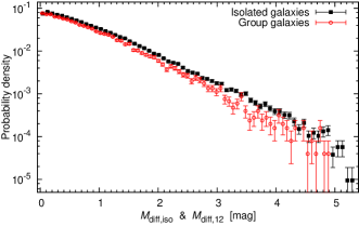
Figure 8: The differential distributions of magnitude differences for group first-ranked and second-ranked galaxies (open circles) and of magnitude differences between isolated galaxies and the faint limit of the visibility window (filled squares).

The overall similarity of both distributions suggests that our assumption (that isolated galaxies are actually the first-ranked galaxies with fainter companions located outside the observational window) passes the magnitude difference test. Of course, this test does not exclude the possibility of existence of truly isolated galaxies.

4.3 Group visibility at different distances

As a further test to check our hypothesis concerning the nature of isolated galaxies we check how well actual nearby groups are visible, if shifted to larger distances. For this purpose we selected two subsamples of groups at different true distances from the observer (and with different mean absolute magnitude of the first-ranked group galaxy, $M_{1}$). The first subsample was chosen in a nearby region with distances $100\leq d<200$ $h^{-1}$ Mpc, and the number of visible galaxies $N_{\mathrm{gal}}\geq 10$. The other group sample was chosen in the distance interval $200\leq d<300$ $h^{-1}$ Mpc, and $N_{\mathrm{gal}}\geq 10$.

Figure 9: Upper panel: the mean number of galaxies in shifted groups as a function of distance. Lower panel: restored mean total luminosities of shifted groups. The solid line shows the results for groups located initially at distances $100\leq d<200$ $h^{-1}$ Mpc; dashed line – for groups of initial distances $200\leq d<300$ $h^{-1}$ Mpc.

Figure 10: The restored luminosities of shifted groups, in units of the actual luminosity at the true distance.

Next groups were shifted to progressively larger distances, galaxy apparent magnitudes were calculated, and galaxies inside the visibility window were selected. Details of this procedure were described by T06. The number of galaxies inside the visibility window for shifted groups decreases; the mean number of galaxies in shifted groups is shown in the upper panel of Fig. 9. We see that the mean number decreases almost linearly in the $\log N$ - $d$ diagram; at the far side of our survey the mean number of remaining galaxies in groups is between 1 and 2.

The expected total luminosity of groups, calculated on the basis of galaxies inside the visibility window and using the procedure outlined in Sect. 5.2 below, is shown on the lower panel of Fig. 9. We see that the mean values of restored total luminosity of groups are almost identical with the true luminosity at the initial distance. At the very far end, the expected total luminosities of groups are a little higher than the initial luminosity, i.e. the expected luminosities are slightly over-corrected. Lower mean luminosities at low distances are caused by the lower number of groups in this region. The restored luminosities of individual groups have a scatter that increases with distance, as seen from Fig. 10. Luminosities in Fig. 10 are in units of the actual luminosity at the true distance. We plotted in this Figure the expected total luminosities for 30 groups, selected in the region 100–200 $h^{-1}$ Mpc, as a function of shifted distance. This scatter can be used to estimate errors of estimated total luminosities of groups as a function of the number of remaining galaxies in groups.

4.4 Luminosity functions of brightest+isolated galaxies

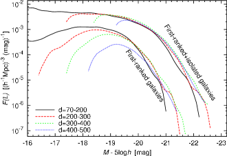
Figure 11: The LFs of the first-ranked and first-ranked+isolated galaxies in different distance intervals (distances are in units of $h^{-1}$ Mpc). The LFs of first-ranked galaxies are shifted to left by 1 mag.

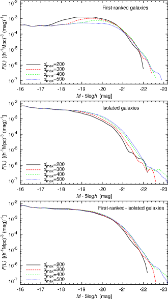
Figure 12: The differential LFs of first-ranked (upper panel), isolated (middle panel) and first-raked+isolated (lower panel) galaxies for samples of different maximum distances ($d_{\mathrm{max}}=200,300,400,500$ $h^{-1}$ Mpc).

To test the assumption that isolated galaxies are first-ranked galaxies, we can also examine how distance-dependent selection effects influence the LFs of first-ranked galaxies and isolated galaxies.

Table 3: Numbers of galaxies in distance-dependent samples

Distance intervala	First-ranked gal.	Isolated gal.	Fractionb
70–200	5184	16724	0.24
200–300	6931	22928	0.23
300–400	7450	28930	0.20
400–500	3888	22426	0.15

^a

Distances are in units $h^{-1}$ Mpc.

^b

Fraction of first-ranked galaxies in the first-ranked+isolated sample.

Figure 11 shows the LFs of first-ranked and first-ranked+isolated galaxies in different distance intervals. The numbers of first-ranked and isolated galaxies in each distance interval are given in Table 3. The LFs of first-ranked galaxies are distance-dependent: with increasing distance the number of faint galaxies decreases. If we add the isolated galaxy sample (we assume that isolated galaxies are first-ranked galaxies) to the first-ranked sample, then the combined LFs are almost independent of distance. The remaining differences are only in the lowest luminosity ranges where data are incomplete; the differences are much smaller than for the first-ranked samples.

In the second test, we calculated the LFs of first-ranked galaxy, isolated and first-ranked+isolated galaxies for a number of limiting distances from the observer: $d_{\mathrm{max}}=200$, 300, 400 and 500 $h^{-1}$ Mpc. The minimum distance is the same for all samples (70 $h^{-1}$ Mpc). The total number of first-ranked galaxies in these subsamples is 5184, 12115, 19565 and 23453, respectively.

The calculated LFs are shown in Fig. 12. If we look only at the first-ranked or the isolated galaxy samples, then the LFs depend on distance. If we combine these two samples, then the combined LFs are independent of distance. This supports our assumption that most of isolated galaxies are actually the first-ranked galaxies with satellite galaxies outside the visibility window. With increasing distance, the fraction of (visible) brightest galaxies decreases (see Table 3). With increasing environmental density, the fraction of first-ranked galaxies increases (see Table 2).

Our tests show that all (or almost all) bright isolated galaxies are actually first-ranked galaxies. We cannot say that for fainter galaxies: there might be some fainter galaxies that are truly isolated.

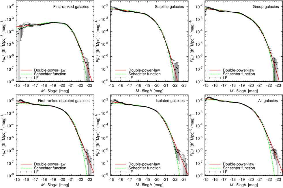
Figure 13: Differential LFs for various galaxy populations: first-ranked, satellite, first-ranked+satellite (group), first-ranked+isolated, isolated and all galaxies. The points are LFs, using 2dF galaxy catalogue. Error-bars are Poisson 1-$\sigma$ errors. The red solid line is the double-power-law and the green dashed line is the Schechter function.

5 Full luminosity functions

5.1 Comparison of the Schechter and the double-power-law luminosity functions

A double-power-law form of the group LF was found already by Christensen (1975); Kiang (1976); Abell (1977); Mottmann & Abell (1977). In these papers a sharp transition between two power indices at a characteristic luminosity $L^{*}$ was applied. We shall use a smooth transition:

$$F(L)\mathrm{d}L\propto(L/L^{*})^{\alpha}(1+(L/L^{*})^{\gamma})^{(\delta-\alpha)/\gamma}\mathrm{d}(L/L^{*}),$$ (5)

where $\alpha$ is the exponent at low luminosities $(L/L^{*})\ll 1$, $\delta$ is the exponent at high luminosities $(L/L^{*})\gg 1$, $\gamma$ is a parameter that determines the speed of transition between the two power laws, and $L^{*}$ is the characteristic luminosity of the transition, similar to the characteristic luminosity of the Schechter function. A similar double-power law was also used by Vale & Ostriker (2004) to fit the mass-luminosity relation in their subhalo model, and by Cooray & Milosavljević (2005a) to fit the luminosity function of central galaxies.

We shall compare the double-power-law function with the popular Schechter (1976) function:

$$F(L)\mathrm{d}L\propto(L/L^{*})^{\alpha}\exp{(-L/L^{*})}\mathrm{d}(L/L^{*}),$$ (6)

where $\alpha$ and $L^{*}$ (or the respective absolute magnitude $M^{*}$) are parameters.

Table 4: Schechter and double-power-law parameters

	Schechter		Double-power-law
Sample	$\alpha$	$M^{*}$	$\alpha$	$\gamma$	$\delta$	$M^{*}$
First-ranked galaxies	$-0.557\pm 0.031$	$-19.95\pm 0.04$	$-0.802\pm 0.015$	$2.44\pm 0.13$	$-6.22\pm 0.40$	$-20.97\pm 0.07$
Satellite galaxies	$-1.131\pm 0.026$	$-19.18\pm 0.04$	$-1.231\pm 0.031$	$1.73\pm 0.19$	$-7.95\pm 1.84$	$-20.44\pm 0.31$
Group galaxies	$-1.197\pm 0.020$	$-19.96\pm 0.04$	$-1.177\pm 0.044$	$1.23\pm 0.19$	$-8.43\pm 3.53$	$-21.44\pm 0.72$
First-ranked+Isolated	$-1.031\pm 0.016$	$-19.93\pm 0.03$	$-1.211\pm 0.013$	$2.14\pm 0.14$	$-5.64\pm 0.48$	$-20.69\pm 0.11$
Isolated galaxies	$-1.058\pm 0.017$	$-19.76\pm 0.03$	$-1.258\pm 0.013$	$2.37\pm 0.17$	$-5.35\pm 0.41$	$-20.43\pm 0.10$
All galaxies	$-1.098\pm 0.012$	$-19.77\pm 0.02$	$-1.200\pm 0.022$	$1.66\pm 0.15$	$-5.71\pm 0.71$	$-20.60\pm 0.20$
Groups	$-0.928\pm 0.020$	$-22.05\pm 0.04$	$-0.734\pm 0.045$	$0.89\pm 0.10$	$-5.98\pm 0.76$	$-23.33\pm 0.60$

$M^{*}$ is in units of mag$-5\log(h)$.

Figure 13 presents the LFs for various galaxy populations: first-ranked , satellite, first-ranked+satellite (group), first-ranked+isolated, isolated and all galaxies. When calculating LFs, we have selected galaxies from all density regions. The LFs have a well-defined bend around $L^{*}\simeq 10^{10}\,h^{-2}\mathrm{L}_{\sun}$ ($M^{*}-5\log h\simeq-20$), and an almost constant level for luminosities $M^{*}-5\log h>-19$: the LFs slightly increase by moving toward lower luminosities, except for the first-ranked galaxy sample, where the LF is decreasing.

For all galaxy populations we have fitted the Schechter and double-power-law functions for these LFs. The Schechter and double-power-law parameters with error estimates for each sample are given in Table 4. In general, both functions give a pretty good fit. Since the double-power-law has more free parameters, the fit is slightly better. There is still one big difference between the Schechter and the double-power-law: for most populations, the Schechter law predicts too few bright galaxies; the double-power-law gives a much better fit for the bright end of the LF and a better fit in the bend region.

5.2 Determination of expected total luminosities of groups

The main problem in the calculation of the group LF is the reduction of observed group luminosities to expected total luminosities which take into account galaxies outside the visibility window. The 2dFGRS is a flux-limited survey, since very bright as well as faint galaxies cannot be observed for redshifts using the multifibre technique. The estimated total luminosity by T06 was found using the Schechter (1976) LF of galaxies, as done also by Moore et al. (1993); Tucker et al. (2000).

In calculating the luminosities of groups we regard every galaxy as a visible member of a density enhancement within the visible range of absolute magnitudes, $M_{1}$ and $M_{2}$, corresponding to the observational window of apparent magnitudes, $m_{1}$ and $m_{2}$, at the distance of the galaxy. This assumption is based on observations of nearby galaxies, which indicate that practically all galaxies are located in systems of galaxies of various size and richness. In this paper we came to similar conclusions that truly isolated galaxies are rare, and most observed isolated galaxies are actually the first-ranked galaxies.

To estimate the expected total luminosity of groups we assume that the LFs derived for a representative volume can be applied also for individual groups and galaxies. Under this assumption the estimated total luminosity per one visible galaxy is

$$L_{\mathrm{tot}}=L_{\mathrm{obs}}W_{L},$$ (7)

where $L_{\mathrm{obs}}=\mathrm{L}_{\sun}10^{0.4\times(M_{\sun}-M)}$ is the luminosity of the visible galaxy of absolute magnitude $M$ (in units of the luminosity of the Sun, $\mathrm{L}_{\sun}$), and

$$W_{L}={\frac{\int_{0}^{\infty}L\,F(L)\mathrm{d}L}{\int_{L_{1}}^{L_{2}}L\,F(L)\mathrm{d}L}}$$ (8)

is the luminous-density weight (the ratio of the expected total luminosity to the expected luminosity in the visibility window). $L_{1}$ and $L_{2}$ are lower and upper limit of the luminosity window, respectively. In our calculations we have adopted the absolute magnitude of the Sun in the $b_{J}$ filter $M_{\sun}=5.33$ (Eke et al. 2004b). Further we have adopted the $k\!+\!e$-correction according to Norberg et al. (2002).

In T06 paper we used the Schechter function for calculating the weights. In this paper we use the double-power-law instead of the Schechter one, as the double-power-law represents better the bright end of the LFs. For weights, we use the double-power-law derived from the full galaxy sample. The weights assigned to galaxies as a function of distance from the observer are shown in Fig. 14. At a distance $d\approx 100$ $h^{-1}$ Mpc weights are close to unity; here the observational window of apparent magnitudes covers the absolute magnitude range of the majority of galaxies. Weights rise toward very small distances due to the influence of bright galaxies outside the observational window, which are not numerous but are very luminous. At larger distances the weight $W_{L}$ rises again due to the influence of faint galaxies outside the observational window. The fairly large scatter of weights at any given distance is due to differences of the $k\!+\!e$-correction for galaxies of various energy distribution parameter $\eta$, and the scatter of the incompleteness correction.

Figure 14: The weights used to correct for invisible galaxies outside the observational luminosity window.

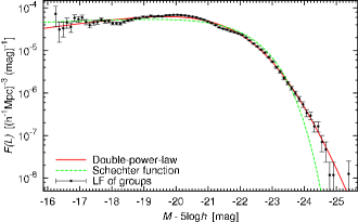
Figure 15: The differential LF of groups (shown by points). The red solid line is the double-power-law fit and the green dashed line is the Schechter function.

As we have the total luminosities of groups, we are able to calculate the group LF. It is plotted in Fig. 15. Compared with the galaxy LF, the turn-off is shifted toward brighter luminosities and the LF is shallower. Here again, the Schechter function predicts too few bright groups. The Schechter and double-power-law parameters for the group LF are given in Table 4.

6 Discussion

6.1 Distribution of groups in various environments

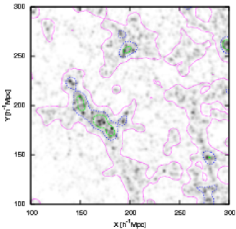
Figure 16: The projected luminosity density distribution of the central area of the 2dFGRS Northern sample. The green long-dashed line surrounds the supercluster core region, the blue dashed line – the supercluster region, and the dotted violet line – the filament region, the rest is the void region. The luminous supercluster near the center of the Figure is SCL126, according to the catalogue by Einasto et al. (1997).

To visualise the environmental dependence of the LFs we show in Fig. 16 a 2-D luminosity density distribution in different regions of the global density. We show a slice of the 2dFGRS with a thickness of 100 $h^{-1}$ Mpc  at a distance $d=250$ $h^{-1}$ Mpc, perpendicular to the line-of-sight, with suitably chosen Cartesian coordinates within the plane of the slice. We see that in supercluster and their core regions there are numerous dense knots – rich clusters of galaxies. Knots (clusters/groups) in filament regions form elongated clouds around superclusters; often these clouds continue filaments inside superclusters. The most luminous supercluster seen in this Figure is SCL126. It is connected with neighbouring superclusters by numerous filaments.

6.2 Evolution of groups in various environments

To understand the differences between group LFs we performed an analysis of evolution of haloes (simulated groups) in different global environments. For this purpose we simulated the evolution of a model universe with standard cosmological parameters $\Omega_{\mathrm{m}}=0.27$, $\Omega_{\Lambda}=0.73$, $\sigma_{8}=0.84$, $z_{\mathrm{init}}=500$, $N_{\mathrm{part}}=N_{\mathrm{grid}}=256^{3}$ in a box of size $L=256$ $h^{-1}$ Mpc. Particle positions and velocities were stored for epochs $z=100$, 50, 20, 10, 5, 2, 1, 0.5 and 0. The density field was calculated for all epochs using two smoothing kernels, the Epanechnikov kernel of the radius of 8 $h^{-1}$ Mpc, and the Gaussian kernel of the rms width of 0.8 $h^{-1}$ Mpc. These fields define the global and local environment, respectively. For the present epoch the high-resolution density field was used to find compact haloes. The haloes were defined as all particles within a box $\pm 2$ cells around the cell of the peak local density. All together 41060 haloes were found. For each halo its position, peak local density, global environmental density at its location, and mass were stored; the mass was found by counting the number of particles in groups (the mass of each particle is $7.487\times 10^{10}\,\mathrm{M}_{\sun}$). For all haloes particle identification numbers were stored, so it was easy to find positions of particles of present-epoch haloes at earlier epochs.

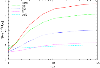
Figure 17: The evolution of the size of samples of particles, collected in haloes at the present epoch, as a function of redshift $z$. Present time haloes have been selected in regions of different global density at the present epoch, corresponding to supercluster cores, superclusters, filaments of various global density, and in voids.

To follow changes of the size of the clouds of particles in present-day haloes we calculated the mean sizes of particle clouds for earlier epochs. In the present study we are not interested in the changes of positions of groups during their evolution, thus we found the mean position of each halo and its sizes along three coordinate directions; the mean of these sizes was taken as the size of the halo. Halo samples for this study were collected in 5 global density regions at the present epoch, which correspond to cores of superclusters, superclusters, rich and poor filaments, and voids. This division corresponds approximately to observed group populations located in various global density environments, studied above.

The changes of mean sizes of model haloes located in various global environment are presented in Fig. 17. The Figure shows dramatic differences in the evolution of halo sizes. Haloes in void regions have almost identical sizes over the whole time interval used in this study. In contrast, the sizes of haloes in present core regions of superclusters were much larger at earlier epochs: the sizes have decreased by a factor of about 5. In regions of intermediate global density the changes are the smaller, the lower is the environmental density.

These differences in the evolution of halo mean sizes are mainly due to differences in the merger history of haloes in various environments. In high-density regions the present-day haloes are collected from numerous smaller haloes formed independently around the present brightest group. During this process the mass of the halo increases. The merger rate is a function of the environmental density, thus we observe gradual changes of the LFs of first-ranked galaxies.

The masses of haloes at the present epoch as a function of the global environmental density are shown in Fig. 18. For a given environmental density the masses have a well-defined upper limit, which increases over two orders of magnitude when we move from the void environment to the supercluster core environment. As argued by Einasto et al. (1994), this has a simple explanation. In all regions where the density is below average, the density decreases continuously and there is no possibility to form compact objects – galaxies. In regions where the density is above the average, it increases until matter collapses to form haloes. The growth of density is the more rapid the higher is the density. This is the usual gravitational instability process; for a recent simulation of that see, e.g., Gao et al. (2005).

Figure 18: The masses of haloes in regions of different global density at the present epoch. Haloes have been found by the FoF method using the same model as in Fig. 17.

Similar halo evolution histories in various environments were recently constructed by Romeo et al. (2008), using detailed hydrodynamical simulations. Empirical evidence for differences in galaxy evolution comes among other sources also from the Millennium Galaxy Catalogue, see Driver et al. (2006).

6.3 Comparison with earlier studies

The LF of group brightest and satellite galaxies was investigated recently by a number of authors. Yang et al. (2008a) used the Data Release 4 of the Sloan Digital Sky Survey to study the LF in the framework of a long series of papers devoted to the halo occupation distribution (van den Bosch et al. 2003; Yang et al. 2003, 2004; van den Bosch et al. 2004, 2005; Zheng et al. 2005; Yang et al. 2005b; van den Bosch et al. 2008, and references in Yang et al. (2008a)). Similar studies were made also by Tinker et al. (2005); Cooray & Cen (2005); Cooray & Milosavljević (2005a); Milosavljević et al. (2006); Tinker et al. (2006); Vale & Ostriker (2006); Tinker et al. (2007); Hansen et al. (2007); Tinker & Conroy (2008); Vale & Ostriker (2008).

Hansen et al. (2007); Yang et al. (2008a) found that luminosities of first-ranked galaxies of rich groups have a relatively small dispersion (see Fig. 5 of Hansen et al. (2007) and Fig. 2 of Yang et al. (2008a)). In their halo occupation model Cooray & Milosavljević (2005a) use for central galaxies a double-power-law model with a sharp decline at low luminosities, depending on the mass of the halo. Thus new data confirm the earlier results by Hubble & Humason (1931); Hubble (1936); Sandage (1976); Postman & Lauer (1995) and many others. In most of these studies only very rich groups were considered. In our study also poorer groups were investigated, and we found that they have a lower low-luminosity limit in dense environments than rich groups do. Cooray & Milosavljević (2005a); Yang et al. (2008a) showed that the median luminosity of first-ranked galaxies depends strongly on the mass of the halo (group). To compare with their results we plot in the lower panel of Fig. 19 the luminosities of first-ranked galaxies as a function of the estimated group total luminosity. The median luminosity of first-ranked galaxies is shown by a red line. Our results are very close to those by Yang et al., see their Fig. 6 (left panel). Yang et al. use as argument the estimated group (halo) mass, which is closely related to the estimated total luminosity. Our study shows also that the median luminosity and the width of the luminosity distribution of first-ranked galaxies depend on the density of the environment.

These results mean that first-ranked galaxies of groups located in a dense environment have a rather well fixed lower luminosity limit. The decrease of the LF at low luminosities was noticed in the NGC901/902 supercluster by Wolf et al. (2005) for dust-free old galaxies (their Fig. 11).

One of important results of the present study is the finding about the nature of isolated galaxies in a flux-limited sample: most isolated galaxies are actually the first-ranked galaxies, where the fainter members of groups lie outside the visibility window. A similar result was obtained by Yang et al. (2008a) using the halo occupation model. Arguments used in our study and by Yang et al. are very different, so both studies complement each other.

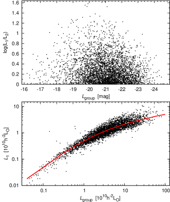
Figure 19: Upper panel: The luminosity gap between the first-ranked and second-ranked galaxies in groups, $\log L_{1}-\log L_{2}$, as a function of the first-ranked galaxy luminosity. The lower panel shows the luminosity of the first-ranked galaxy as a function of the total estimated luminosity of the group. The red line shows the median luminosity.

Yang et al. (2008a) also studied the gap between the first-ranked and second-ranked galaxies. Their results show that the width for the gap lies in range $\log(L_{1}/L_{2})=0.0$–$0.6$. For our groups, the width of the gap is even larger (see the upper panel of Fig. 19). This Figure shows that the gap has the highest values for medium rich groups of a total expected luminosity about $L_{\mathrm{group}}=2\times 10^{10}\leavevmode\nobreak\ h^{-2}\mathrm{L}_{\odot}$, i.e. for groups of the type of the Local Group. Milosavljević et al. (2006) used the luminosity gap statistic to investigate the cluster merger rate and to define “fossil” groups.

Cross et al. (2001) determined a bivariate brightness distribution of a subsample of 2dFGRS, i.e. the joint surface brightness-luminosity distribution. Their analysis shows that if the surface brightness is taken into account, then more exact extrapolation of the expected total galaxy luminosity is possible. This results in a shift of the characteristic magnitude $M^{*}$ brightwards by 0.33 mag, and in an increase of the total estimated number density of galaxies by a factor of about 1.2. The normalization of the LF for the Millennium Galaxy Catalogue was discussed by Liske et al. (2003); Cross et al. (2004); Driver et al. (2005), where normalization parameters for various previous determinations of the LF were found. In this paper we are comparing the LFs of first-ranked galaxies, second-rank, and isolated galaxies. As the shifts found by Cross et al. and Liske et al. influence these populations approximately in the same manner, we expect that our results are insensitive to the surface brightness effect.

An extensive study of LFs in various environments using the 2dF Galaxy Redshift Survey was made by Croton et al. (2005). Their main results are the same that we found. Using the halo occupation model Mo et al. (2004) and Tinker & Conroy (2008) argue that the dependence of the LF on the large-scale environment is determined by differences in the masses of DM haloes. Our simple model shows that in different global environments the masses of DM haloes may differ by orders of magnitude, see Fig. 18, in agreement with Mo et al. and Tinker & Conroy results. Semi-analytic models also predict that void galaxies should be fainter than galaxies in dense regions (Benson et al. 2003; Tinker & Conroy 2008, see also Einasto et al. (2005)).

In general, all studies show that as we move from high density regions to low density regions (voids), galaxies become fainter. Interestingly, our study shows that in high density environments (supercluster core regions), all LFs are different from those in other environments. This result is new, although the decrease of the LF at low luminosities was noticed in the NGC901/902 supercluster by Wolf et al. (2005) for dust-free old galaxies. It is difficult to explain this effect with selection effects since, as seen also in Fig. 16, the galaxies in supercluster core regions in the area plotted here are located at the same distances as galaxies in the nearby lower density regions where also low luminosity galaxies are seen. We believe that in cores of rich superclusters the faintest galaxies have been swallowed by the brightest galaxies/groups, since in high density environments merger events are much more common. The reason why this has not been found in other studies, is probably a different definition of the high density environment. Cores of rich superclusters are specific regions that contain clusters and groups of galaxies, as well as isolated galaxies, and may contain X-ray clusters of galaxies. The morphology of supercluster cores differ from the morphology of supercluster outskirts (Einasto et al. 2008). Thus supercluster cores are not just an environment that contains groups of galaxies (groups may be located also in poor superclusters), and the LFs of galaxies in supercluster cores are not the same as the LFs of galaxy clusters (see, for example, Hansen et al. (2007)). The supercluster environment (excluding cores) can also be considered as a high density environment but here the galaxy and group content differs from that in core regions. Thus here the definition of the environment is crucial.

Our study does not include very faint galaxies, as, for example, the study of the core region of the Shapley supercluster (Mercurio et al. 2006). Thus future work is needed to understand the difference between the faint ends of the LFs in our and Mercurio et al. study.

One difference between the earlier studies and our work lies in the use of the analytical LFs. Most earlier authors have used the Schechter function, but our results show that this function is not good to describe the bright end of the LF. This difficulty was noticed already by Blanton et al. (2005) using the SDSS data. They also showed that the Schechter function does not fit the LF of extremely low luminosity galaxies. In a Shapley Supercluster region Mercurio et al. (2006) conclude that the bright end of the Schechter function is not sufficient to fit the data. Yang et al. (2008a) also use different analytical expressions of LFs for different populations: a log-normal distribution for first-ranked galaxies, and a modified Schechter function for satellite galaxies. The difficulty of the use of the standard Schechter function for satellite galaxies lies in the fact that the slope of the LF at high luminosities is much steeper than in the standard case where the slope is fixed by the exponential law. The double-power-law LF overcomes both difficulties and can be used for brightest as well as for satellite galaxies. This difference is crucial in cases where only very bright galaxies are visible, at the far end of flux-limited samples. Here small differences in the accepted analytical LF can lead to large differences in the expected total luminosities of groups.

Hoyle et al. (2005) studied the SDSS void galaxies. Their faint end slope of the LF is comparable to our results ($\alpha=-1.0$–$-1.3$). They also conclude that the faint-end slope is not strongly dependent on the environment, at least up to group densities. This is in agreement with our results, where the faint-end slope is almost the same for all populations, except for the first-ranked galaxy. However, in our samples there are still small changes when moving from voids to superclusters: the faint-end slope is steeper for void galaxies, and becomes flatter when moving toward higher densities. Our faint-end slope $\alpha$ for the galaxy LF is in range $-1.0$–$-1.3$ (except for the first-ranked galaxy), that is in good agreement with observations and models (see e.g. Baldry et al. 2005; Xia et al. 2006; Khochfar et al. 2007; Liu et al. 2008).

6.4 Interpretation of the luminosity function

By definition, the transition of the power laws from low luminosities to high luminosities occurs at a luminosity approximately equal to the characteristic luminosity $L^{*}$, see Fig. 13 and Table 4. The luminosity $L^{*}$ corresponds also to the median luminosity of first-ranked galaxies when averaged over various environments (except the void environment), see Fig. 7. Fig. 6 and Table 1 of Yang et al. (2008a) show similar coincidences for groups (haloes) of various masses.

Cooray & Milosavljević (2005b) demonstrated that the LF of galaxies can be calculated in the halo model using two premises: 1) the luminosities of central galaxies have a lognormal distribution, $L^{*}$ being the mean luminosity of central galaxies in massive haloes; and 2) the luminosities of satellite galaxies are distributed as a power law. These assumptions mean that the high-luminosity section of the LF is determined by the first-ranked galaxies, and the low-luminosity section – by the conditional LF of luminosity differences of satellite galaxies from the luminosity of the brightest galaxy.

Properties of the LF of various types of galaxies in different environments can be interpreted by differences of galaxy and group evolution. In supercluster cores rich groups form through many mergers, thus the second-ranked galaxies have been brightest galaxies of poorer groups before they have been absorbed into a larger group. In lower-density environment the merger rate is lower and groups of galaxies have been collected only from nearby regions through minor mergers and continuous infall of matter to galaxies as suggested by White & Rees (1978). Gas infall to galaxies (haloes) is very different in various environments, as shown by hydrodynamical simulations by Kereš et al. (2005). The satellite LF contains also information on the galaxy formation feedback, see Cooray & Cen (2005).

7 Conclusions

We used the 2dF Galaxy Redshift Survey to derive the LF of different samples: the brightest (first-ranked ), second-ranked, satellite and isolated galaxies and the LF of groups. We studied the LFs for various environments. The principal results of our study are the following:

• The LFs of galaxies (for all samples) are strongly dependent on the environment, in agreement with earlier studies.

• In the highest density regions (supercluster cores) the LFs for all galaxy populations have a well-defined lower luminosity limit, about $10^{9}\mathrm{L}_{\sun}$. Here the first-ranked galaxies have larger luminosities than the first-ranked galaxies in other regions, in concordance with several earlier studies.

• In the lowest density regions (voids) the LFs are shifted in respect to the LFs of all other regions, toward lower luminosities. Here, and in filament regions, the LFs of first-ranked galaxies have a plateau at the faint end.

• The LF of second-ranked galaxies in high-density regions is similar to the LF of first-ranked galaxies in lower-density regions. The bright end of the LF of satellite galaxies is almost identical with the bright end of the LF of second-ranked galaxies. At lower luminosities the LF of satellite galaxies lies higher than the LF of second-ranked galaxies.

• Almost all bright isolated galaxies can be identified with first-ranked galaxies where the remaining galaxies lie outside the observational window used in the selection of galaxies for the survey. Truly isolated galaxies are rare; they are faint and are located mainly in voids.

• The LF of galaxies and groups can be expressed by a double-power-law more accurately than by the Schechter function. The biggest differences are in the bright end of the LF, where the Schechter function predicts too few bright galaxies. The advantage of double-power-law is clearly visible for the LF of groups.