Possibility of Detecting Moons of Pulsar Planets Through Time-of-Arrival Analysis

Abstract

The perturbation caused by planet-moon binarity on the time-of-arrival signal of a pulsar with an orbiting planet is derived for the case in which the orbits of the moon and the planet-moon barycenter are both circular and coplanar. The signal consists of two sinusoids with frequency $(2n_{p}-3n_{b})$ and $(2n_{p}-n_{b})$, where $n_{p}$ and $n_{b}$ are the mean motions of the planet and moon around their barycenter, and the planet-moon system around the host, respectively. The amplitude of the signal is equal to the fraction $\sin I[9(M_{p}M_{m})/16(M_{p}+M_{m})^{2}][r/R]^{5}$ of the system crossing time $R/c$, where $M_{p}$ and $M_{m}$ are the the masses of the planet and moon, $r$ is their orbital separation, $R$ is the distance between the host pulsar and planet-moon barycenter, $I$ is the inclination of the orbital plane of the planet, and $c$ is the speed of light. The analysis is applied to the case of PSR B1620-26 b, a pulsar planet, to constrain the orbital separation and mass of any possible moons. We find that a stable moon orbiting this pulsar planet could be detected, if the moon had a separation of about one fiftieth of that of the orbit of the planet around the pulsar, and a mass ratio to the planet of $\sim$ 5% or larger.

1 Introduction to Extra-solar Moons

In the past decade and a half, over two hundred and fifty extra-solar planets have been discovered. With the data expected to be produced by satellites such as COROT (Auvergne et al., 2003) and Kepler (Basri, Borucki & Kock, 2005), it will not only be possible to find smaller planets, but moons of those planets as well (Szabó et al., 2006). As a result, the detectability of extra-solar moons is starting to be explored in terms of their effect on planetary microlensing (Han & Han, 2002) and transit lightcurves (Sartoretti & Schneider, 1999; Szabó et al., 2006). Upper limits have already been placed on the mass and radius of putative moons of the planets HD 209458 b (Brown et al., 2001), OGLE-TR-113 b (Gillon et al., 2006) and HD 189733 b (Pont et al., 2007).

While the limitations of microlensing and the transit technique for detecting moons have been discussed and used in the literature, the limitations of other techniques such as the time-of-arrival (TOA) technique have not. This technique involves determining the variations in line-of-sight position to the host star, usually a pulsar, using the observed time of periodic events associated with that host. The aim of this analysis is to explore exactly what the TOA signal of a planet-moon pair is, and relate it to the planetary systems that can give the most precise timing information, the systems around millisecond pulsars.

2 Review of Planetary Detection Around Millisecond Pulsars

The first planetary system outside the Solar System was detected around the millisecond pulsar PSR 1257+12 (Wolszczan & Frail, 1992). This detection was made by investigating periodic variations in the time of arrival of its radio pulses using a timing model. An example timing model for the case in which the planet’s orbit around the pulsar is circular is:

$$\left(t_{N}-t_{0}\right)=\left(T_{N}-T_{0}\right)+\Delta T_{corr}+TOA_{pert,p}(M_{s},M_{p},R,I,\phi_{b}(0)),$$ (1)

where $t_{0}$ and $t_{N}$ are the times at which the initial and $N^{th}$ pulses are emitted in the pulsar’s frame, $T_{0}$ and $T_{N}$ are the times the initial and $N^{th}$ pulses are received in the observatory’s frame, and the term $\Delta T_{corr}$ acts to change the frame of reference from the observatory on Earth to the barycenter of the pulsar system (see Backer, 1993, for a more complete discussion of the components of $\Delta T_{corr}$). The final term represents the effect of a planet on the motion of the pulsar, where $R$ is the planet-pulsar distance, $I$ is the angle between the normal of the planet-pulsar orbit and the line-of-sight and $\phi_{b}(0)$ is the initial angular position of the planet measured from the $x$-axis, about the system barycenter. In addition, $M_{s}$ and $M_{p}$ are the mass of the pulsar and the planet, respectively.

Currently, four planets around two millisecond pulsars have been discovered, three around PSR 1257+12 (Wolszczan & Frail, 1992; Wolszczan, 1994) and one around PSR B1620-26 (Backer, Foster & Sallmen, 1993). These four planets include one with mass $~{}0.02$ Earth masses, the lowest mass extra-solar planet known. This low-mass detection threshold, in addition to measurements of orbital perturbations (e.g., the 2:3 orbital resonance between PSR 1257+12c and PSR 1257+12d, Konacki & Wolszczan, 2003), demonstrate the sensitivity of the TOA technique. Indeed, as a result of their high rotation rate (and thus large number of sampled pulses) and low level of noise activity, millisecond pulsars make optimal targets for high precision TOA work (see e.g., Cordes, 1993).

3 What is the TOA Perturbation Caused by a Moon?

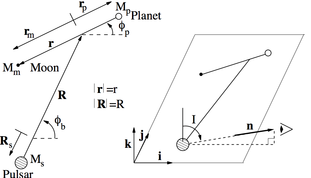
Figure 1: Coordinate system used in the analysis of the TOA perturbation caused by a moon. The subscripts s, b, p and m refer to the pulsar, planet-moon barycenter, planet and moon, respectively. The diagram on the left shows the quantities used to describe the position of the three bodies in their mutual orbital plane, while the diagram on the right shows the relationship between this orbital plane and the observer.

In order to investigate the perturbation caused by planet-moon binarity, the timing model presented in equation (1) must be updated to include effects due to the presence of the moon. For simplicity, we consider here only systems in which both the orbit of the planet and moon around their common barycenter, and the orbit of the planet-moon barycenter around the pulsar, are both circular and lie in the same plane. An example model taking this assumption into account is:

$$\left(t_{N}-t_{0}\right)=\left(T_{N}-T_{0}\right) + \Delta T_{corr}+TOA_{pert,p}(M_{s},M_{p}+M_{m},R,I,\phi_{b}(0))$$ (2)

$$+ TOA_{pert,pm}(M_{s},M_{p},M_{m},r,R,I,\phi_{b}(0),\phi_{p}(0)).$$

We have explicitly modified $TOA_{pert,p}$ to indicate that it depends on the combined planet-moon mass, and included another term, $TOA_{pert,pm}$, to account for planet-moon binarity. Here $M_{m}$ is the mass of the moon, $r$ is the distance between the planet and the moon, and $\phi_{p}(0)$ is the initial angular position of the planet measured from the planet-moon barycenter. The quantities $R$, $r$, $I$, $\phi_{b}$ and $\phi_{p}$ are shown in Figure 1. The functional form of $TOA_{pert,pm}$ can be derived from $\mathbf{R}_{s}$, the vector between the system barycenter and the pulsar, using:

$$\frac{1}{c}\int_{0}^{t}\int_{0}^{t^{\prime}}\mathbf{\ddot{R}}_{s}\cdot\mathbf{n}dt^{\prime\prime}dt^{\prime}=TOA_{pert,p}+TOA_{pert,pm},$$ (3)

where $c$ is the speed of light and $\mathbf{n}$ is a unit vector pointing along the line of sight, the only direction along which quantities can be measured.

The governing equation for $\mathbf{R_{s}}$ can be written as the sum of the zeroth order term, which describes $TOA_{pert,p}$, and the tidal terms, which describe $TOA_{pert,pm}$:

$$\frac{d^{2}\mathbf{R}_{s}}{dt^{2}} = \frac{G(M_{p}+M_{m})}{R^{3}}\mathbf{R}$$ (4)

$$+ \left[-\frac{G(M_{p}+M_{m})}{R^{3}}\mathbf{R}+\frac{GM_{p}}{\left|\mathbf{R}+\mathbf{r}_{p}\right|^{3}}(\mathbf{R}+\mathbf{r}_{p})+\frac{GM_{m}}{\left|\mathbf{R}+\mathbf{r}_{m}\right|^{3}}(\mathbf{R}+\mathbf{r}_{m})\right],$$

where the tidal terms have been collected into square brackets and noting that $\mathbf{R}_{s}=-(M_{p}+M_{m})/(M_{s}+M_{p}+M_{m})\mathbf{R}$, $\mathbf{r}_{p}=-M_{m}/(M_{p}+M_{m})\mathbf{r}$ and $\mathbf{r}_{m}=M_{p}/(M_{p}+M_{m})\mathbf{r}$, and where the vectors $\mathbf{R}_{s}$, $\mathbf{R}$, $\mathbf{r}_{p}$, $\mathbf{r}_{m}$ and $\mathbf{r}$ are also shown in Figure 1. Using the coordinate system in Figure 1, it can be seen after some algebra that:

$$\mathbf{R}+\mathbf{r}_{m} = \left[R\cos\phi_{b}-\frac{M_{p}}{M_{p}+M_{m}}r\cos\phi_{p}\right]\mathbf{i}+\left[R\sin\phi_{b}-\frac{M_{p}}{M_{p}+M_{m}}r\sin\phi_{p}\right]\mathbf{j}$$ (5)

$$\mathbf{R}+\mathbf{r}_{p} = \left[R\cos\phi_{b}+\frac{M_{m}}{M_{p}+M_{m}}r\cos\phi_{p}\right]\mathbf{i}+\left[R\sin\phi_{b}+\frac{M_{m}}{M_{p}+M_{m}}r\sin\phi_{p}\right]\mathbf{j}$$ (6)

where $\mathbf{i}$ and $\mathbf{j}$ are defined in Figure 1, and $\mathbf{i}$ is the direction to the line-of-sight, projected onto the plane of the orbit.

As the orbits are both circular and coplanar, we have that $\phi_{b}(t)=n_{b}t+\phi_{b}(0)$, and $\phi_{p}(t)=n_{p}t+\phi_{p}(0)$ where $n_{b}$ and $n_{p}$ are the constant mean motions of the two respective orbits. Substituting equations (5) and (6) into the coefficients of the last two terms of equation (4), assuming $r\ll R$ and using the binomial expansion to order $r^{2}/R^{2}$ gives:

$$\frac{GM_{m}}{\left|\mathbf{R}+\mathbf{r}_{m}\right|^{3}} = \frac{GM_{m}}{R^{3}}\left[1+3\frac{M_{p}}{(M_{m}+M_{p})}\frac{r}{R}\cos(\phi_{b}-\phi_{p})\right.$$ (7)

$$\left.+\frac{M_{p}^{2}}{(M_{m}+M_{p})^{2}}\frac{r^{2}}{R^{2}}\left(-\frac{3}{2}+\frac{15}{2}\cos^{2}(\phi_{b}-\phi_{p})\right)\right]$$

$$\frac{GM_{p}}{\left|\mathbf{R}+\mathbf{r}_{p}\right|^{3}} = \frac{GM_{p}}{R^{3}}\left[1-3\frac{M_{m}}{(M_{m}+M_{p})}\frac{r}{R}\cos(\phi_{b}-\phi_{p})\right.$$ (8)

$$\left.+\frac{M_{m}^{2}}{(M_{m}+M_{p})^{2}}\frac{r^{2}}{R^{2}}\left(-\frac{3}{2}+\frac{15}{2}\cos^{2}(\phi_{b}-\phi_{p})\right)\right].$$

Substituting equations (5), (6), (7) and (8) into (4) gives, after simplification:

$$\frac{d^{2}\mathbf{R}_{s}}{dt^{2}} = \frac{G(M_{p}+M_{m})}{R^{3}}\mathbf{R}+\frac{GM_{p}M_{m}}{(M_{m}+M_{p})}\frac{r^{2}}{R^{4}}\left[\left(-\frac{3}{2}+\frac{15}{2}\cos^{2}(\phi_{b}-\phi_{p})\right)\right.$$ (9)

$$\Biggl{.}\times\left(\cos\phi_{b}\mathbf{i}+\sin\phi_{b}\mathbf{j}\right)-3\cos(\phi_{b}-\phi_{p})\left(\cos\phi_{p}\mathbf{i}+\sin\phi_{p}\mathbf{j}\right)\Biggr{]}.$$

From Figure 1 it can be seen that:

$$\mathbf{n}=\sin I\mathbf{i}+\cos I\mathbf{k}.$$ (10)

Substituting equations (9) and (10) into equation (3), gives:

$$TOA_{pert,pm} = \frac{-\sin I\ GM_{p}M_{m}}{c(M_{m}+M_{p})}\frac{r^{2}}{R^{4}}\left[\frac{3}{4n_{b}^{2}}\cos\phi_{b}+\frac{3}{8(n_{b}-2n_{p})^{2}}\cos(\phi_{b}-2\phi_{p})\right.$$ (11)

$$\left.+\frac{15}{8(3n_{b}-2n_{p})^{2}}\cos(3\phi_{b}-2\phi_{p})\right].$$

The $\cos\phi_{b}$ term in equation (11) has the same frequency as the signal of a lone planet and it can be shown that it acts to increase the measured value of $M_{p}+M_{m}$ derived from $TOA_{pert,p}$ by $(3/4)(r^{2}/R^{2})(M_{p}M_{m}/(M_{p}+M_{m}))$. Consequently, this term can be neglected as it will be undetectable as a separate signal. Also, the edge of the stability region for a prograde satellite of the low-mass component of a high-mass binary can be approximated by $0.36r_{H}$ for the case of circular orbits, where $r_{H}=R\left[(M_{p})/(3M_{s})\right]^{1/3}$ is the secondary’s Hill radius (Holman & Wiegert, 1999). When $r$ is equal to this maximum stable radius $n_{p}\approx 8n_{b}$. As $n_{b}\ll n_{p}$ is likely, we have that the denominators of the $\cos(\phi_{b}-2\phi_{p})$ and $\cos(3\phi_{b}-2\phi_{p})$ terms will never approach zero. This, in addition to the assumption of zero eccentricities, means that resonance effects can be neglected. Consequently, equation (11) can be simplified by neglecting $n_{b}$ in the denominators, giving:

$$TOA_{pert,pm}=\frac{-\sin IGM_{p}M_{m}}{c(M_{m}+M_{p})}\frac{r^{2}}{R^{4}}\left[\frac{3}{32n_{p}^{2}}\cos(\phi_{b}-2\phi_{p})+\frac{15}{32n_{p}^{2}}\cos(3\phi_{b}-2\phi_{p})\right].$$ (12)

Writing $n_{p}$ in terms of $r$, using Kepler’s law, gives:

$$TOA_{pert,pm}=-\sin I\frac{M_{p}M_{m}}{(M_{m}+M_{p})^{2}}\frac{R}{c}\left(\frac{r}{R}\right)^{5}\left[\frac{3}{32}\cos(\phi_{b}-2\phi_{p})+\frac{15}{32}\cos(3\phi_{b}-2\phi_{p})\right].$$ (13)

From equation (13), we have that the size of the perturbation varies as $[M_{m}M_{p}/(M_{m}+M_{p})^{2}][r/R]^{5}$ times the system crossing time, $R/c$. So, the best hope of a detectable signal occurs when the planet-moon pair are close to the parent pulsar, widely separated from each other, both quite massive, and very accurate timing data is available.

Our result is consistent with a similar study done by Schneider & Cabrera (2006), who calculated the radial velocity perturbation on one component of a binary star system for the case in which the other component was an unresolved pair. Converting their radial velocity perturbation to a timing perturbation, setting the mass of the planet and moon equal to each other, as in the case investigated by Schneider & Cabrera (2006), and noting that $r$ in this work is equivalent to their $2a_{A}$, our formula and that of Schneider & Cabrera (2006) agree.

4 Is is Possible to Detect Moons of Planets Orbiting Millisecond Pulsars?

To investigate whether or not it is possible to detect moons of pulsar planets, we simplify equation (13) by summing the amplitudes of the sinusoids, giving the maximum possible amplitude:

$$max\left(TOA_{pert,pm}\right)=\frac{9\sin I}{16}\frac{M_{m}M_{p}}{(M_{m}+M_{p})^{2}}\frac{R}{c}\left(\frac{r}{R}\right)^{5}.$$ (14)

Thus, for a given $r/R$, the maximum amplitude increases linearly with $R$. So, for planet-moon pairs that are far from each other and their parent pulsar, detection may be possible. For example, a 0.1AU Jupiter-Jupiter binary located 5.2AU from a host pulsar would produce a $TOA_{pert,pm}$ of amplitude 960ns, which compares well with the 130ns residuals obtained from one of the most stable millisecond pulsars, PSR J0437-4715 (van Straten et al., 2001).

To demonstrate this method, the expected maximum signals from a moon orbiting each of the four known pulsar planets was explored. It was found that in the case of PSR B1620-26 b, signals that are in principle detectable could confirm or rule out certain configurations of moon mass and orbital parameters (see Figure 2).

In the particular case of PSR B1620-26 b, the perturbation signal will not exactly match the signal shown in equation (13) due to the effect of its white dwarf companion. The effect of this companion was investigated as a side project and it was found that its effect was to introduce additional perturbations on top of the $TOA_{pert,p}$ and $TOA_{pert,pm}$ calculated. Consequently, the detection threshold represents an upper limit to the minimum detectable signal and thus the analysis is still valid.

Figure 2: The regions of parameter space containing detectable (shaded) and stable (cross-hatched) moons of the planet PSR B1620-26 b are shown as a function of planet-moon separation and moon mass. The total mass and the distance of the planet-moon pair from the parent pulsar were assumed to be 2.5 Jupiter masses and 23AU respectively (Sigurdsson et al., 2003), while it was assumed that $\sin I=1$. The mass of the host was set at 1.7 solar masses (the sum of the mass of the pulsar and its white dwarf companion). The $3\sigma$ detection threshold was calculated assuming the $\sim 40\mu s$ timing residuals given in Thorsett et al. (1999) are uncorrelated and that similar accuracy TOA measurements of PSR B1620-26 continue to the present day. The stability region was estimated as 0.36 times the Hill sphere of the planet.

Unfortunately, there are practical limits to the applicability of this method. They include discounting other systems that could produce similar signals, sensitivity limits due to intrinsic pulsar timing noise, and limits imposed by moon formation and stability.

First, other systems that could produce similar signals need to be investigated. Possible processes include pulsar precession (see e.g., Akgün, Link & Wasserman, 2006), periodic variation in the ISM (Scherer et al., 1997), gravitational waves (Detweiler, 1979), unmodelled interactions between planets (Laughlin & Chambers, 2001) and other small planets. To help investigate the last two options, we plan on completing a more in-depth analysis of the perturbation signal of an extra-solar moon, including the effects of orbital inclination and orbital eccentricity.

Second, the noise floor of the system needs to be examined. The suitability of pulsars for signal detection is limited by two main noise sources, phase jitter and red timing noise (for example, Cordes, 1993). Phase jitter is error due to pulse-to-pulse variations and leads to statistically independent errors for each TOA measurement. Phase jitter decreases with increasing rotation rate (decreasing $P$) due to the resultant increase in the number of pulses sampled each integration. Red timing noise refers to noise for which neigbouring TOA residuals are correlated. Red timing noise has been historically modeled as a random walk in phase, frequency or frequency derivative (for example, Boynton et al., 1972; Groth, 1975; Cordes, 1980; Kopeikin, 1997). Red noise is strongly dependent on $\dot{P}$. This relationship can be understood from the theoretical standpoint that red noise is due to non-homogeneous angular momentum transport either between components within the pulsar (e.g. Jones, 1990) or between it and its environment (e.g. Cheng, 1987). To illustrate the effect of these two noise sources on TOA accuracy, an estimate of their combined residuals as a function of $P$ and $\dot{P}$ is shown in Figure 3. For comparison, the values of $P$ and $\dot{P}$ of every pulsar as of publication are also included. The ATNF Pulsar Catalogue (Manchester et al., 2005) was used to provide the pulsar data for this plot.

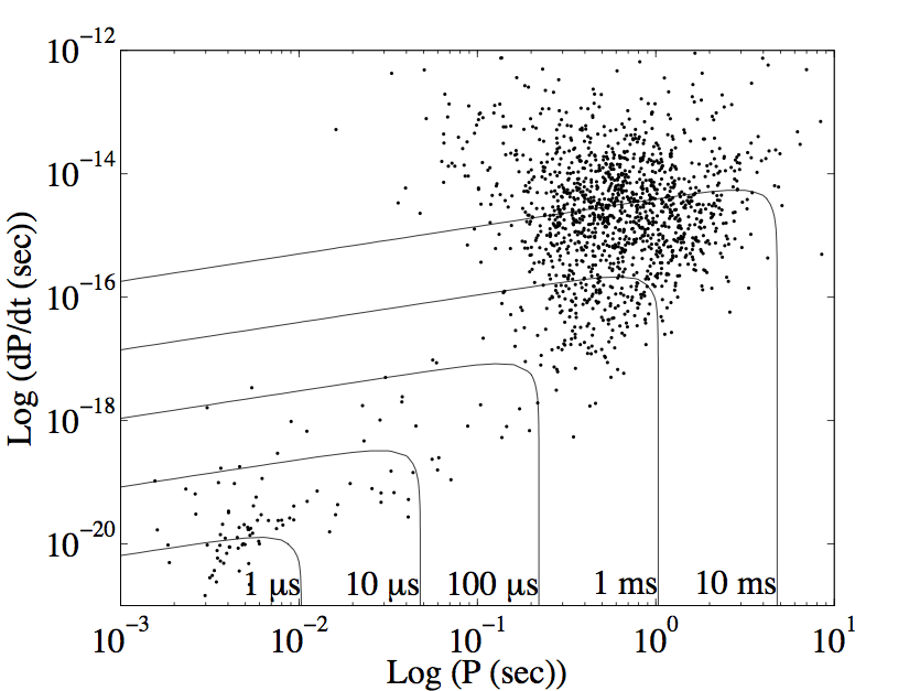
Figure 3: Contour plot of predicted timing noise as a function of pulsar rotation period and period derivative. For comparison, all known pulsars as of publication are overplotted. This plot is based on Figure 9 from Cordes (1993). Consequently, the functions and assumptions used to generate the contours are the same as given in Cordes (1993), noting that that each TOA integration is 1000 seconds long. As the correlated timing noise measured for individual pulsars can vary from the predicted values by two orders of magnitude (see e.g., Arzoumanian et al., 1994), this plot is meant to demonstrate global pulsar properties, not predict individual pulsar noise characteristics.

Third, whether or not moons will be discovered depends on whether or not they exist in certain configurations, which depends on their formation history and orbital stability. Recent research suggests that there are physical mass limits for satellites of both gas giants (Canup & Ward, 2006) and terrestrial planets (Wada & Kokubo, 2006). Also, tidal and three-body effects can strongly affect the longevity of moons (Barnes & O’Brien, 2002; Domingos, Winter & Yokohama, 2006; Atobe & Ida, 2007).

Finally, while this method was investigated for the specific case of a pulsar host, this technique could also be applied to planets orbiting other clock-like hosts such as pulsating giant stars (Silvotti et al., 2007) and white dwarfs (Mullally, Winget & Kepler, 2006).

References

- Akgün et al. (2006) Akgün T., Link B., Wasserman I., 2006, MNRAS, 365, 653
- Arzoumanian et al. (1994) Arzoumanian Z., Nice D. J., Taylor J. H. & Thorsett S. E., 1994, ApJ, 422, 671
- Atobe & Ida (2007) Atobe K., & Ida S., 2007, Icarus, 188, 1
- Auvergne et al. (2003) Auvergne M., et al., 2003, Proc. SPIE, 4854, 170
- Backer (1993) Backer, D. C., 1993, PASP, 36, 11
- Backer et al. (1993) Backer D. C., Foster R. S., & Sallmen S., 1993, Nature, 365, 817
- Barnes & O’Brien (2002) Barnes J. W. & O’Brien D. P., 2002, ApJ, 575, 1087
- Basri et al. (2005) Basri G., Borucki W. J., & Kock D., 2005, New A Rev., 49, 478
- Boynton et al. (1972) Boynton, P. E., Groth, E. J., Hutchinson, D. P., Nanos, G. P., Jr., Partridge, R. B., & Wilkinson, D. T., 1972, ApJ, 175, 217
- Brown et al. (2001) Brown T. M., Charbonneau D., Gilliland R. L., Robert L., Noyes R. W. & Burrows A., 2001, ApJ, 552, 699
- Canup & Ward (2006) Canup R. M. & Ward W. R., 2006, Nature, 441, 834
- Cheng (1987) Cheng K. S., 1987, ApJ, 321, 805
- Cordes (1980) Cordes J. M., 1980, ApJ, 237, 216
- Cordes (1993) Cordes J. M., 1993, PASP, 36, 43
- Detweiler (1979) Detweiler, S., 1979, ApJ, 234, 1100
- Domingos et al. (2006) Domingos R. G., Winter O. C. & Yokohama T., 2006, MNRAS, 373, 1227
- Gillon et al. (2006) Gillon M., Pont F., Moutou C., Bouchy F., Courbin F., Sohy S. & Magain P., 2006, A&A, 459, 249
- Groth (1975) Groth, E. J., 1975, ApJS, 29, 443
- Han & Han (2002) Han C., & Han W., 2002, ApJ, 580, 490
- Holman & Wiegert (1999) Holman M. J. & Wiegert P. A., 1999, AJ, 117, 621
- Jones (1990) Jones P. B., 1990, MNRAS, 246, 364
- Kopeikin (1997) Kopeikin S. M., 1997, MNRAS, 288, 129
- Konacki & Wolszczan (2003) Konacki M., & Wolszczan A., 2003, ApJ, 591, L147
- Laughlin & Chambers (2001) Laughlin G., & Chambers J. E., 2001, ApJ, 551, L109
- Manchester et al. (2005) Manchester R. N., Hobbs G. B., Teoh A., & Hobbs M., 2005, ApJ, 129, 1993
- Mullally et al. (2006) Mullally F., Winget D. E., & Kepler S. O., 2006, PASP, 352, 265
- Pont et al. (2007) Pont F. et al., 2007, A&A, 476, 1347
- Sartoretti & Schneider (1999) Sartoretti P., & Schneider J., 1999, Ap&SS, 134, 553
- Scherer et al. (1997) Scherer K., Fichtner H., Anderson J. D., & Lau E. L., 1997, Science, 278, 1919
- Schneider & Cabrera (2006) Schneider J. & Cabrera J., 2006, A&A, 445, 1159
- Sigurdsson et al. (2003) Sigurdsson S., Richer H., Hansen B., Stairs I. & Thorsett S., 2003, Science, 301, 193
- Silvotti et al. (2007) Silvotti et al., 2007, Nature, 449, 189
- Szabó et al. (2006) Szabó Gy. M., Szátmary K., Divéki Zs., & Simon A., 2006, A&A, 450, 395
- Thorsett et al. (1999) Thorsett S. E., Arzoumanian Z., Camilo F., Lyne A. G., 1999, ApJ, 523, 763
- van Straten et al. (2001) van Straten W., Bailes M., Britton M., Kulkarni S. R., Anderson S. B., Manchester R. N., & Sarkissian J., 2001, Nature, 412, 158
- Wada & Kokubo (2006) Wada K., & Kokubo E., 2006, ApJ, 638, 1180
- Wolszczan (1994) Wolszczan A., 1994, Science, 264, 538
- Wolszczan & Frail (1992) Wolszczan A., & Frail D. A., 1992, Nature, 355, 145