Remote atom entanglement in a fiber-connected three-atom system

Abstract

An Ising-type atom-atom interaction is obtained in a fiber-connected three-atom system. The interaction is effective when $\Delta\approx\gamma_{0}\gg g$. The preparations of remote two-atom and three-atom entanglement governed by this interaction are discussed in specific parameters region. The overall two-atom entanglement is very small because of the existence of the third atom. However, the three-atom entanglement can reach a maximum very close to $1$.

I Introduction

Generating the entanglement between spatially separated atoms plays an important role in quantum information processing and quantum computation, such as quantum storage^[1], quantum key distribution^[2] and quantum states swapping^[3]. To efficiently entangle two or more distant atoms, one must create some kind of direct or indirect interaction between them, such as by adopting appropriate measurement on optical fields that conditionally interact with atoms and thereby the atoms (as a subsystem) can be projected to an entangled state, or by using quantum-correlated fields interacting with atoms and thereby the entanglement among the fields can be transferred to atoms. Based upon this, a variety of schemes for entangling distant atoms or distant photons have been proposed recently^[4-14]. For example, fascinating schemes have been presented to efficiently entangle distant atoms, where the single-photon interference effect was applied with^[4] or without^[5] weak driving laser pulse. Recently, S. Mancini and S. Bose proposed a novel scheme to directly entangle two atoms trapped in distant cavities^[6] which were connected via optical fibers. Using input-output theory, under adiabatic approximation, the authors obtained an effective Ising model for two atoms. In their scheme, photon acted as an intermediate quantum information carrier and mapped the quantum information from the atom in one cavity to that in another. Such systems are meaningful not only in quantum measurement or testing Bell's inequalities but also in potential applications such as quantum encryption^[15] or constructing universal quantum gates^[16] that are essential for designing quantum network. Nevertheless, in discussing quantum networking with trapped atoms and photons in cavity QED system^[17], two problems should be overcome: How to generate the entanglement of a N-atom system? What is the exact influence of the collective interaction on the entanglement shared by remote atoms? These problems have been discussed intensively, for instance in the scheme proposed by Cabrillo et al^[4]. The simplest multi-atom case is a three-atom system which might be an intuitive extension from a two-atom case. In our scheme, We extend the model of two-atom circumstance in Ref. [6] to three-atom which turns out to be a three-atom Ising model. Such an approach might be meaningful in discussing the above problems for multiple distant atoms. We firstly investigate the dependence of the effective Ising coupling coefficients on the atom-cavity detuning and cavity leakage. Then, we discuss the influence of an atom on the other two atoms entanglement properties. Furthermore, we study the characters of remote three-atom entanglement and the tangle between one atom and the rest two atoms.

II Optical fibers connected three-atom system

The schematic setup for our system is shown in Fig. 1. Three identical two-level atoms 1, 2 and 3 are trapped in spatially distant cavities $C_{1}$, $C_{2}$ and $C_{3}$ respectively. All the cavities are assumed to be single-sided ones. Three off-resonant external driving field $\varepsilon_{1}$, $\varepsilon_{2}$ and $\varepsilon_{3}$ are applied upon cavity $C_{1}$, $C_{2}$ and $C_{3}$ respectively. In each cavity, a local laser field that is resonantly coupled to the atom is applied. Two neighboring cavities are connected via optical fibers. Apparently, the subsystem constituted by cavities $C_{1}$ and $C_{2}$ or $C_{2}$ and $C_{3}$ is just the setup proposed in Ref. [6].

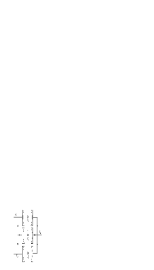
Figure 1: Schematic setup of the system. Three two-level atoms locate in spatially separated single-sided optical cavities that are connected via optical fibers.

In the interaction picture, using cavity input-output theory^[18] and taking adiabatic approximation^[19], we obtain an effective Hamiltonian for this system as (see Appendix A)

$$H_{eff}=J_{12}\sigma_{1}^{z}\sigma_{2}^{z}+J_{23}\sigma_{2}^{z}\sigma_{3}^{z}+J_{31}\sigma_{3}^{z}\sigma_{1}^{z}+\sum\limits_{i}\Gamma_{i}(\sigma_{i}^{+}+\sigma_{i}^{-}),$$ (1)

which is a three-particle Ising chain with magnetic fields perpendicular to the $z$ direction^[20], $J_{12}$ and $J_{23}$ represent the nearest-neighbor (NN) atoms coupling coefficients, while $J_{31}$ represents next-nearest-neighbor (NNN) atoms interaction strength. $\sigma_{i}^{z}(i=1,2,3)$ is spin operator of atom $i$, $\sigma_{i}^{+}(\sigma_{i}^{-})$ is atomic raising (lowering) operators. $\Gamma_{i}$ is the magnitude of the locally applied laser field interacting with atom $i$. We define

$$J_{12}= 2\gamma_{0}\chi^{2}Im\left\{\alpha_{1}\alpha_{2}^{\ast}e^{i\phi_{21}}/[M^{2}-W^{2}]\right\},$$

$$J_{23}= 2\gamma_{0}\chi^{2}Im\left\{\alpha_{3}\alpha_{2}^{\ast}e^{i\phi_{32}}/[M^{2}-W^{2}]\right\},$$

$$J_{31}= 2\gamma_{0}\chi^{2}Im\left\{\gamma_{0}\alpha_{3}\alpha_{1}^{\ast}e^{i(\phi_{23}+\phi_{12})}/[M(M^{2}-W^{2})]\right\},$$ (2)

where $\gamma_{0}$ is the cavity leakage rate, $\chi=g^{2}/\Delta$, $g$ is the coupling strength between the atom and the cavity field in cavity $C_{i}$, $\Delta$ is the detuning between the atomic internal transition and cavity field frequency, where, large detuning approximation has been assumed, i.e. $\Delta\gg g$, and $M=i\Delta+\gamma_{0}$, $W^{2}=\gamma_{0}^{2}\left[e^{i(\phi_{21}+\phi_{12})}+e^{i(\phi_{32}+\phi_{23})}\right]$. The phase factors $\phi_{ij}(ij=12,21,23,32)$ are caused from the photons transmission along optical fibers from cavity $C_{j}$ to cavity $C_{i}$^[21]. Physically, they depend on the frequency of the photons and the distance between cavities. And

$$\alpha_{1} =\frac{\varepsilon_{1}M^{2}+\varepsilon_{2}M\gamma_{0}e^{i\phi_{12}}+\gamma_{0}^{2}[\varepsilon_{3}e^{i\Theta_{13}}-\varepsilon_{1}e^{i\Phi_{1}}]}{M(M^{2}-W^{2})},$$

$$\alpha_{2} =\frac{\varepsilon_{2}M+\gamma_{0}(\varepsilon_{1}e^{i\phi_{21}}+\varepsilon_{3}e^{i\phi_{23}})}{M^{2}-W^{2}},$$

$$\alpha_{3} =\frac{\varepsilon_{3}M^{2}+\varepsilon_{2}M\gamma_{0}e^{i\phi_{32}}+\gamma_{0}^{2}[\varepsilon_{1}e^{i\Theta_{31}}-\varepsilon_{3}e^{i\Phi_{3}}]}{M(M^{2}-W^{2})},$$ (3)

where $\Theta_{13}=\phi_{12}+\phi_{23},\Phi_{1}=\phi_{23}+\phi_{32},\Theta_{31}=\phi_{32}+\phi_{21},\Phi_{3}=\phi_{21}+\phi_{12}$. The global system is now determined by a series of independent parameters as $\varepsilon_{1},\varepsilon_{2},\varepsilon_{3},\Delta,\gamma_{0},\phi_{12},\phi_{32},\Gamma_{1},\Gamma_{2}$ and $\Gamma_{3}$. In next section, we discuss the optimal region of the parameters for the preparation of remote atom entanglement.

III Parameters space description of Ising coupling coefficients

From Eqs. (3), the condition $M^{2}\approx W^{2}$ leads to large Ising coupling coefficients. This condition also keeps the validity of the adiabatic approximation in case of weak local laser fields, i.e. $J_{12}(J_{23},J_{31})\gg\Gamma_{i},i=1,2,3$. We can further simplify the condition as

$$\phi_{21}+\phi_{12}\approx\phi_{23}+\phi_{32}\approx\frac{\pi}{2},\Delta\approx\gamma_{0}.$$ (4)

For simplicity, we assume $\varepsilon_{1}=\varepsilon_{2}=\varepsilon_{3}=\varepsilon_{0}$, $\Gamma_{1}=\Gamma_{2}=\Gamma_{3}=\Gamma_{0}$. The parameters space can now be expressed in unit of $g$ as $(\Delta/g,\gamma_{0}/g)g$. In Fig. 2-3, we give the description of Ising coupling coefficients for NN and NNN atoms in the parameters space. Where we assume $\varepsilon_{0}=2g$. We can see that the coupling coefficients for NN atoms as well as NNN atoms can be divided into two regions: (a) the region where $\Delta>\gamma_{0}$, (b) the region where $\Delta<\gamma_{0}$. In most area of the two regions, the coupling coefficients are very small, only in the regions just besides the line $\Delta=\gamma_{0}$ are they large enough so that the validity of the adiabatic approximation can be kept.

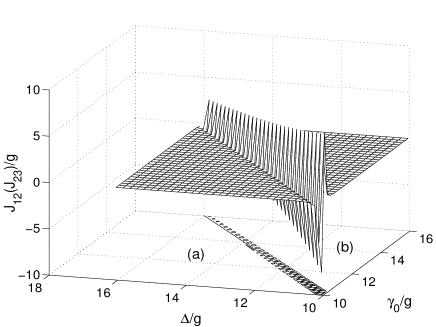
Figure 2: The amount of NN atoms coupling coefficients($J_{12}(J_{23})$) under different detuning ($\Delta$) and cavity leakage rate ($\gamma_{0}$). All the variables are presented in unit of $g$.

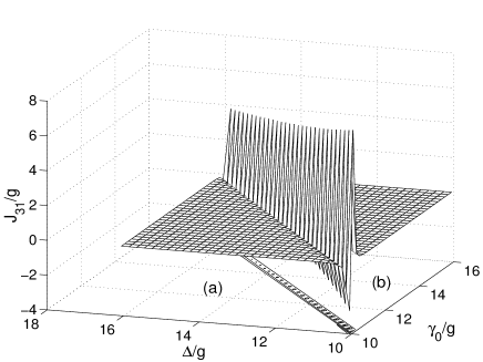
Figure 3: The amount of NNN atoms coupling coefficients($J_{31})$ under different detuning ($\Delta$) and cavity leakage rate ($\gamma_{0}$). All the variables are presented in unit of $g$.

In the following discussions, we will study two-atom entanglement nature and three-atom entanglement properties based on the parameter space.

IV Nearest-neighbor and next-nearest-neighbor remote two-atom entanglement

In this section, we discuss the nature of remote two-atom subsystem entanglement which is generated in our system. Wootters proposed a general measurement for the amount of two-qubit (noted as 1 and 2) entanglement. It is named as Concurrence^[22]:

$$C_{12}=\max\{0,\lambda_{1}-\lambda_{2}-\lambda_{3}-\lambda_{4}\},$$ (5)

where $\lambda_{i}$ are the non-negative square roots of the four eigenvalues of non-Hermitian matrix $\rho_{12}\tilde{\rho}_{12}$ with $\tilde{\rho}_{12}$ defined as $(\sigma_{y}\otimes\sigma_{y})\rho^{\ast}_{12}(\sigma_{y}\otimes\sigma_{y})$, where $\rho_{12}$ is the density matrix of the two-qubit system.

We depict the two-atom entanglement situation in Fig. 4-5 for different parameter spaces. We assume that all the atoms are initially in their ground state, so that $|\psi(0)\rangle=|g\rangle_{1}\otimes|g\rangle_{2}\otimes|g\rangle_{3}$.

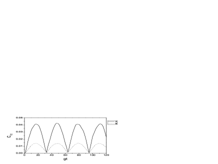
Figure 4: Entanglement of atom 1 and 2 versus time for A: (solid line) $J_{31}\approx 1.2g$, B: (dotted line) $J_{31}\approx-1.2g$. Where we assume $\Gamma_{0}=0.1g$.

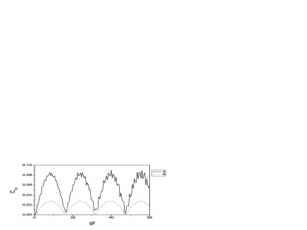
Figure 5: Descriptions are same as those in Fig. 4 but for $\Gamma_{0}=0.2g$. Note that the whole time scale is half of that in Fig. 4.

Firstly, we investigate the influence of $J_{31}$ on the entanglement of NN atoms. In Fig. 4, we adopt appropriate values of $\Delta$ and $\gamma_{0}$ (which satisfy the condition in Eq. (4)) and assume $\Gamma_{0}=0.1g$. The Ising coupling coefficients are $J_{12}=J_{23}\approx-2.4g$, $J_{31}\approx 1.2g$ for solid line, and $J_{31}\approx-1.2g$ for dotted line. If all the signs of the coefficients are reversed, the resulting concurrences are not changed. Evidently, relative larger entanglement for NN atoms can be obtained when $J_{12}(J_{23})\cdot J_{31}<0$. While, compared with the result in Ref. [6], the overall entanglement is very weak since two-atom subsystem is in mixed state during the evolution.

In addition, the NN atoms entanglement can be manipulated through the alternating of the locally applied laser fields. In Fig. 5, we adopt the same parameters as those in Fig. 4 but for $\Gamma_{0}=0.2g$. Fig. 5 indicates that, the increase of $\Gamma_{0}$ remarkably improves the NN atoms entanglement. The period is depressed, but the amount of entanglement is much enhanced. The amount of entanglement for NNN atoms, under the parameters we assumed, is generally much weaker than NN atoms. To improve the entanglement for NNN atoms, The Ising coupling coefficient between NNN atoms must be enhanced. In Fig. 6, we depict the entanglement for NNN atoms. Correspondingly, $J_{12}=J_{23}=-2.4g$, $J_{31}=1.2g$. To modulate the entanglement, we let $\Gamma_{2}=0$. Under this circumstance, the entanglement for NNN atoms can compare with that for NN atoms (see Fig. 4).

Figure 6: Entanglement of atom 1 and 3 versus time when the laser field applied in cavity $C_{2}$ is turn off, that is $\Gamma_{1}=\Gamma_{3}=0.3g$, $\Gamma_{2}=0$.

V The remote three-atom entanglement properties

The intrinsic three-partite entanglement which is widely used for measuring three-partite entanglement of pure states is defined as^[23]

$$C_{123}=C_{1(23)}-C_{12}^{2}-C_{13}^{2},$$ (6)

where $C_{1(23)}$, which represents the tangle between a subsystem 1 and the rest of the global system (denoted as $(23)$), is written as

$$C_{1(23)}=4Det\rho_{1}=2(1-Tr\rho_{1}^{2}).$$ (7)

In Fig. 7, we plot the remote three-atom entanglement $C_{123}$(the solid line), the tangle $C_{1(23)}$(the dotted line), and the Concurrence $C_{12}$(the dashed line) for $|\psi(0)\rangle=|g\rangle_{1}\otimes|g\rangle_{2}\otimes|g\rangle_{3}$. Where the corresponding parameters are same as those of the dotted line in Fig. 5. In fact, there is only very little difference between $C_{123}$ and $C_{1(23)}$. To distinguish $C_{1(23)}$ from $C_{123}$, the line of $C_{1(23)}$ is raised to $0.1+C_{1(23)}$.

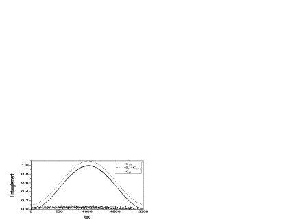
Figure 7: The three-atom entanglement $C_{123}$(solid line), the tangle $C_{1(23)}$(dotted line), and the Concurrence $C_{12}$(dashed line) versus $gt$, where $J_{12}(J_{23})=-2.4g$, $J_{31}=-1.2g$ and $\Gamma_{0}=0.2g$. To distinguish $C_{1(23)}$ from $C_{123}$, the line for $C_{1(23)}$ is raised to $0.1+C_{1(23)}$.

It has been pointed in last section that the Concurrence that represents the bipartite entanglement between atom 1 and atom 2 is very small. While, the tangle, which expresses the entanglement of atom 1 and the rest of the global system, and the remote three-atom entanglement can reach maximum values almost 1 for intermediate values of $gt$. Under the condition of strong Ising coupling coefficients $(J_{12}(J_{23},J_{31})\gg\Gamma_{0})$, if we express the tangle between atom 1 and the rest of the global system as a sum of the remote three-atom entanglement and the bipartite entanglement, the three-atom entanglement will act as the largest contribution. It has been concluded that in a system of $N$ spin-half particles, under the condition of strong Ising coupling coefficients, the $N$-partite entanglement will be dominant^[24].

VI Conclusion

We have obtained a three-atom Ising chain in cavity QED system by connecting three distant cavities via optical fibers. The Ising coupling coefficients are found to be large in the region where $\Delta\approx\gamma_{0}\gg g$, which keeps the validity of the adiabatic approximation. We have discussed the generation of remote atom entanglement. The overall two-atom entanglement is very small because of the existence of the third atom. While, the NN atoms entanglement can be improved when the coupling coefficient of NNN atoms has a contrary sign with respect to that of NN atoms. The locally applied laser fields play an important role in modulating the entanglement quantitatively and qualitatively not only for NN atoms but also for NNN atoms. Furthermore, we have studied the remote three-atom entanglement and the tangle. It is shown that three-atom entanglement, which has a much longer period than two-atom entanglement, can reach a maximum very close to $1$.

In addition, it should be noted that the dissipation of the photon information along the fibers should be investigated, while, the dissipation can be included in the Ising coupling coefficients and act as a decaying exponential factor $e^{-\nu L}$, where $\nu$ is the dissipation rate per meter, $L$ is the total length of the fiber^[25]. The phase factors $e^{i\phi_{12}}$ and $e^{i\phi_{23}}$ are then replaced by $e^{i\phi_{12}-\nu L_{12}}$ and $e^{i\phi_{23}-\nu L_{23}}$. In fact, the dissipative effect along fibers can be compensated by lowering the detuning $\Delta$. One can obtain large Ising coupling coefficients by adopting the parameters in the regions just besides the line $\Delta\approx\sqrt{2e^{-\nu(L_{12}+L_{23})}-1}\gamma_{0}$.

Appendix A

In the interaction picture, the Hamiltonian of the global system can be written as

$$H_{int}=H_{int1}+H_{int2}+H_{int3}+H_{int4},$$

where $H_{int1}$ represents the effective interaction of atoms and cavity fields, $H_{int2}$ is the coupling between external driving fields and cavity fields , $H_{int3}$ represents the interaction of locally applied laser fields and atoms, $H_{int4}$ is the interaction of cavity fields and their environment which is described as a superposition of series of harmonic oscillators. Under the condition of large detuning, we have^[26]

$$H_{int1}=\chi\sum\limits_{i}A_{i}^{+}A_{i}\sigma_{i}^{z},$$

where i=1,2,3, $A_{i}(A_{i}^{+})$ represent cavity fields annihilation (creation) operators in cavities $C_{i}$. And^[18]

$$H_{int2}=\sum\limits_{i}\varepsilon_{i}(A_{i}^{+}+A_{i}),$$ (A3)

$$H_{int3}=\sum\limits_{i}\Gamma_{i}(\sigma_{i}^{+}+\sigma_{i}^{-}).$$ (A4)

We assume $\Gamma_{i}$ are weak enough so that the quantum adiabatic theory^[19] can be applied in the following calculations.

$$H_{int4}=i\int\limits_{-\infty}^{+\infty}d\omega\ {\sum\limits_{i}{\kappa_{C_{i}}[b_{C_{i}}(\omega)A_{i}^{+}+h.c.]}},$$ (A5)

where $b_{C_{i}}(\omega)$, $i=1,2,3$, are the annihilation operators of the harmonic oscillators with frequency $\omega$. $\kappa_{C_{i}}$ are the interaction strengths between cavity $C_{i}$ and the harmonic oscillators. The kinetic equations for cavity field operators turn out to be^[18]

$$\dot{A_{1}} =-(i\Delta+i\chi\sigma_{1}^{z}+\frac{\gamma_{C_{1}}}{2})A_{1}+\sqrt{\gamma_{C_{1}}}A_{1,in}+\varepsilon_{1},$$

$$\dot{A_{2}} =-(i\Delta+i\chi\sigma_{2}^{z}+\frac{\gamma_{C_{1}}}{2})A_{2}+\sqrt{\gamma_{C_{2}}}A_{2,in}+\varepsilon_{2},$$

$$\dot{A_{3}} =-(i\Delta+i\chi\sigma_{3}^{z}+\frac{\gamma_{C_{1}}}{2})A_{3}+\sqrt{\gamma_{C_{3}}}A_{3,in}+\varepsilon_{3},$$ (A6)

where $\gamma_{C_{i}}=2\pi[k_{C_{i}}(\omega)]^{2}$ ($i=1,2,3$). If cavities $C_{1}$ and $C_{2}$ are connected via optical fibers (as shown in Fig. 1), so are cavities $C_{2}$ and $C_{3}$, the input-output conditions should be included, so that^[21]

$$\dot{A_{1}} =-\frac{\gamma_{C_{1}}}{2}A_{1}+\sqrt{\gamma_{C_{1}}}A_{2,out}e^{i\phi_{12}},$$

$$\dot{A_{2}} =-\frac{\gamma_{C_{2}}}{2}A_{2}+\sqrt{\gamma_{C_{2}}}A_{1,out}e^{i\phi_{21}}$$

$$+\sqrt{\gamma_{C_{2}}}A_{3,out}e^{i\phi_{23}},$$

$$\dot{A_{3}} =-\frac{\gamma_{C_{3}}}{2}A_{3}+\sqrt{\gamma_{C_{3}}}A_{2,out}e^{i\phi_{32}}.$$ (A7)

For simplicity, assuming the decay rates $\gamma_{C_{1}}=\gamma_{C_{2}}=\gamma_{C_{3}}=\gamma_{0}$ and taking into account the usual boundary conditions^[18]

$$A_{i,out}+A_{i,in}=\sqrt{\gamma_{0}}A_{i},$$ (A8)

where $i=1,2,3$, we can rewrite the kinetic equations for cavity field operators as

$$\dot{A_{1}} =-MA_{1}-i\chi A_{1}\sigma_{1}^{z}+\sqrt{\gamma_{0}}A_{1,in}$$

$$+e^{i\phi_{12}}(\gamma_{0}A_{2}-\sqrt{\gamma_{0}}A_{2,in})+\varepsilon_{1},$$

$$\dot{A_{2}} =-MA_{2}-i\chi A_{2}\sigma_{2}^{z}+\sqrt{\gamma_{0}}A_{2,in}$$

$$+\sum\limits_{j=1,3}{e^{i\phi_{2j}}(\gamma_{0}A_{j}-\sqrt{\gamma_{0}}A_{j,in})}+\varepsilon_{2},$$

$$\dot{A_{3}} =-MA_{3}-i\chi A_{3}\sigma_{3}^{z}+\sqrt{\gamma_{0}}A_{3,in}$$

$$+e^{i\phi_{32}}(\gamma_{0}A_{2}-\sqrt{\gamma_{0}}A_{2,in})+\varepsilon_{3}.$$ (A9)

To solve these equations explicitly, we firstly obtain the expectation values of cavity field operators through

$$\frac{d\left\langle A_{1}\right\rangle}{dt}=\frac{d\left\langle A_{2}\right\rangle}{dt}=\frac{d\left\langle A_{3}\right\rangle}{dt}=0.$$ (A10)

The steady states for cavity fields in $C_{1}$, $C_{2}$ and $C_{3}$ can be obtained as

$$\alpha_{1} =\frac{\varepsilon_{1}M^{2}+\varepsilon_{2}M\gamma_{0}e^{i\phi_{12}}+\gamma_{0}^{2}[\varepsilon_{3}e^{i\Theta_{13}}-\varepsilon_{1}e^{i\Phi_{1}}]}{M(M^{2}-W^{2})},$$

$$\alpha_{2} =\frac{\varepsilon_{2}M+\gamma_{0}(\varepsilon_{1}e^{i\phi_{21}}+\varepsilon_{3}e^{i\phi_{23}})}{M^{2}-W^{2}},$$

$$\alpha_{3} =\frac{\varepsilon_{3}M^{2}+\varepsilon_{2}M\gamma_{0}e^{i\phi_{32}}+\gamma_{0}^{2}[\varepsilon_{1}e^{i\Theta_{31}}-\varepsilon_{3}e^{i\Phi_{3}}]}{M(M^{2}-W^{2})},$$ (A11)

where $\Theta_{13}=\phi_{12}+\phi_{23},\Phi_{1}=\phi_{23}+\phi_{32},\Theta_{31}=\phi_{32}+\phi_{21},\Phi_{3}=\phi_{21}+\phi_{12}$.

Then, in the regime of strong cavity leakage and large detuning (which lead to $\gamma_{0},\Delta>>\chi$), the kinetic Eqs. (A9) are reformed as the following homogeneous linear equations:

$$\dot{a_{1}} =-Ma_{1}-i\chi\alpha_{1}\sigma_{1}^{z}+\sqrt{\gamma_{0}}a_{1,in}$$

$$+e^{i\phi_{12}}(\gamma_{0}a_{2}-\sqrt{\gamma_{0}}a_{2,in}),$$

$$\dot{a_{2}} =-Ma_{2}-i\chi\alpha_{2}\sigma_{2}^{z}+\sqrt{\gamma_{0}}a_{2,in}$$

$$+\sum\limits_{j=1,3}{e^{i\phi_{2j}}(\gamma_{0}a_{j}-\sqrt{\gamma_{0}}a_{j,in})},$$

$$\dot{a_{3}} =-Ma_{3}-i\chi\alpha_{3}\sigma_{3}^{z}+\sqrt{\gamma_{0}}a_{3,in}$$

$$+e^{i\phi_{32}}(\gamma_{0}a_{2}-\sqrt{\gamma_{0}}a_{2,in}),$$ (A12)

where we have replaced field operators $A_{i}$ with $a_{i}+\alpha_{i}$ (i=1,2,3). In solving Eqs. (A12), one can adiabatically eliminate the effect of vacuum input noise. The resulting cavity field operators are now represented by linear combinations of atomic spin operators $\sigma_{i}^{z}$ (i=1,2,3). Substituting the resulting field operators into Eq. (A1), we get the effective Hamiltonian of the global system in the interaction picture as

$$H_{eff} =J_{12}\sigma_{1}^{z}\sigma_{2}^{z}+J_{23}\sigma_{2}^{z}\sigma_{3}^{z}+J_{31}\sigma_{3}^{z}\sigma_{1}^{z}$$

$$+\sum\limits_{i}\Gamma_{i}(\sigma_{i}^{+}+\sigma_{i}^{-}),$$ (A13)

where $J_{12},J_{23}$ and $J_{31}$ are expressed by Eqs. (2).

In deriving Eq. (A13), we neglect self-energy terms including $\sigma_{i}^{z}$ and self-interaction terms including $(\sigma_{i}^{z})^{2}$ and $(\sigma_{i}^{z})^{3}$ that do not change the initial system state. Also, we eliminate higher order terms that include $\chi^{3}\sigma_{1}^{z}\sigma_{2}^{z}\sigma_{3}^{z}$ since the corresponding coupling coefficients are much weaker than $J_{12}$, $J_{23}$ and $J_{31}$. The typical difference between this Hamiltonian and that in Ref. [6] lies in the third term in Eq. (A13).

References

- (1) van der Wal C H, Eisaman M D, Andre A, Walsworth R L, Phillips D F, Zibrov A S and Lukin M D 2003 Science 301 196
- (2) Inoue K, Waks E and Yamamoto Y 2002 Phys. Rev. Lett. 89 037902
- (3) Kuzmich A and Polzik E S 2002 Phys. Rev. Lett. 85 5639
- (4) Cabrillo C, Cirac J, Garcia-Fernandez P and Zoller P 1999 Phys. Rev. A 59 1025
- (5) Feng X L, Zhang Z M, Li X D, Gong S Q and Xu Z Z 2003 Phys. Rev. Lett. 90 217902
- (6) Mancini S and Bose S 2004 Phys. Rev. A 70 022307
- (7) Li H C, Li X H, Lin X, Lin X M and Yang R C 2007 Chin. Phys. 16 1209
- (8) Fang M F and Tan J 2006 Chin. Phys. 15 2514
- (9) Chimczak G 2005 Phys. Rev. A 71 052305
- (10) Duan L M and Kimble H J 2003 Phys. Rev. Lett. 90 253601
- (11) Guo Y Q, Chen J and Song H S 2006 Chin. Phys. Lett. 23 1088
- (12) SimonC and Irvine W T M 2003 Phys. Rev. Lett. 91 110405
- (13) Zou X B, Pahlke K and Mathis W 2003 Phys. Rev. A 68 024302
- (14) Ficek Z and Tanaś R 2003 quant-ph 0302124
- (15) Ekert A 1991 Phys. Rev. Lett. 67 661
- (16) Zou X B and Mathis W 2005 Phys. Rev. A 71 042334
- (17) Moehring D L, Madsen M J, Younge K C, Kohn R N, Jr P Maunz, Duan L M, Monroe C and Blinov B B 2007 J. Opt. Soc. Am. B 24 300
- (18) Walls D F and Milburn G J 1994 Quantum Optics (Springer: Berlin) p121
- (19) Sanrady M S, Wu L A and Lidar D A 2004 Quantum Information Processing 3 331
- (20) Gunlycke D, Kendon V M and Vedral V 2001 Phys. Rev. A 64 042302
- (21) Wiseman H M and Milburn G J 1994 Phys. Rev. A 49 4110
- (22) Wootters W K 1998 Phys. Rev. Lett. 80 2245
- (23) Coffman V, Kundu J and Wootters W K 2000 Phys. Rev. A 61 052306
- (24) Štelmachovič P and Bužek V 2004 Phys. Rev. A 70 032313
- (25) Tittel W, Brendel J, Gisin B, Herzog T, Zbinden H and Gisin N 1998 Phys. Rve. A 57 3229
- (26) Holland M J, Walls D F and Zoller P 1991 Phys. Rev. Lett. 67 1716