Mesoscopic fluctuations in the spin-electric susceptibility due to Rashba spin-orbit interaction

Abstract

We investigate mesoscopic fluctuations in the spin polarization generated by a static electric field and by Rashba spin-orbit interaction in a disordered 2D electron gas. In a diagrammatic approach we find that the out-of-plane polarization – while being zero for self-averaging systems – exhibits large sample-to-sample fluctuations which are shown to be well within experimental reach. We evaluate the disorder-averaged variance of the susceptibility and find its dependence on magnetic field, spin-orbit interaction, dephasing, and chemical potential difference.

A primary goal in semiconductor spin physics is the control of magnetic moments by electric fields Awschalom et al. (2002); Awschalom and Flatté (2007). One way to achieve this is to make use of the magnetoelectric effect (MEE) Levitov et al. (1985); Edelstein (1990), a spin polarized steady state which emerges from intrinsic ’magnetic’ fields generated by spin-orbit interactions (SOI) and transport. While this MEE has been observed e.g. in n-InGaAs epilayers Kato et al. (2004a, b, 2005) and hole gases Silov et al. (2004), the resulting net polarization is below percent for electron systems Kato et al. (2004a, 2005), and thus much smaller than what has been achieved by optical pumping Kato et al. (2004b); Stich et al. (2007); Meier et al. (2007). Moreover, in a standard two-dimensional electron gas (2DEG), with typical Rashba SOI Bychkov and Rashba (1984), the MEE generates only in-plane spin polarization but no out-of-plane components Edelstein (1990). The latter would be desirable, also since they can be detected more easily e.g. by optical means.

However, these observations apply only to disordered phase-incoherent systems with self-averaging Akkermans and Montambaux (2007). On the other hand, it is well-known that phase-coherence in mesoscopic systems leads to new quantum effects such as conductance fluctuations or weak antilocalization, especially due to intrinsic SOI Altshuler (1985); Altshuler et al. (1991); Lee et al. (1987); Zumbühl et al. (2005); Aleiner and Fal’ko (2001); Miller et al. (2003).

Similarly, mesoscopic spin effects emerge for the MEE when the system becomes phase-coherent. Indeed, focussing on 2DEGs with Rashba SOI, we will show here that the spin-electric susceptibility is subject to strong sample-to-sample fluctuations, and thus individual mesoscopic samples with phase coherence can exhibit a large net spin polarization. Quite remarkably, these strong fluctuations show up not only in the in-plane but also in the out-of-plane spin components. We find that these fluctuations considerably exceed the polarization obtained in self-averaging samples, and since the latter has been successfully measured by optical means Kato et al. (2004a, 2005), the spin fluctuations predicted here should be well within experimental reach. We will see that this strong enhancement is special for Rashba (or Dresselhaus) SOI, and, diagrammatically, it results from a spin vertex renormalization typical for such intrinsic SOI Edelstein (1990); Chalaev and Loss (2005); Duckheim and Loss (2006).

Related effects studied before are local spin fluctuations in metallic conductors due to the extrinsic spin-orbit effect Zyuzin (1990) (as opposed to the intrinsic Rashba SOI Engel et al. (2006)), density of states fluctuations of quantum corrals Walls and Heller (2007), and fluctuations of spin currents in general nanostructures Bardarson et al. (2007) and chaotic quantum dots Bardarson et al. (2007); Krich and Halperin (2008). While thermal spin fluctuations have been observed Oestreich et al. (2005), we are not aware of studies of mesoscopic spin fluctuations due to the MEE as described here.

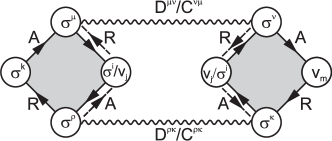
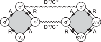
Figure 1: Dominant diagrams (for $1/p_{F}l\ll 1$) leading to the variance $\overline{\delta\chi^{ij}\delta\chi^{km}}$ given in Eq. (Mesoscopic fluctuations in the spin-electric susceptibility due to Rashba spin-orbit interaction), see also Fig. 2. The upper diagram contains the Hikami boxes (HB) $V_{La},V_{Ra}$(with solid arrows and two Diffusons (D)) and $V_{Ld},V_{Rd}$ (with dashed arrows and two Cooperons (C)), resp. The lower diagram contains the HBs $V_{Lb},V_{Rb}$ (solid arrows, two Diffusons) and $V_{Lc},V_{Rc}$ (dashed arrows, two Cooperons).

We consider a disordered mesoscopic square-shaped 2DEG of size $L^{2}$ containing non-interacting electrons of mass $m$ and charge $e$ and described by the Hamiltonian

$$H=\frac{\mathbf{p}^{2}}{2m}+\alpha(p_{1}\sigma^{2}-p_{2}\sigma^{1})+\mathbf{b}\cdot\boldsymbol{\sigma}+V.$$ (1)

Here, $\mathbf{p}=(p_{1},p_{2},0)$ is the in-plane momentum, $\alpha$ the Rashba SOI constant Bychkov and Rashba (1984), $2b=g\mu_{B}B(\cos\varphi_{B},\sin\varphi_{B},0)$ an external in-plane magnetic field, and $\boldsymbol{\sigma}=(\sigma^{1},\sigma^{2},\sigma^{3})$ the Pauli matrices (and $\sigma^{0}=\mathbb{1}$). The disorder potential $V$ is due to static short-ranged impurities randomly distributed and characterized by the mean free path $l=\tau p_{F}/m$, where $\tau$ is the scattering time and $p_{F}$ the Fermi momentum.

The spin polarization due the MEE is given in linear response by $\langle\sigma^{i}\rangle=\chi^{ij}E_{j}$, $i=1,2,3$, where $E_{j}$ is a static electric field applied along the j-direction and $\chi^{ij}$ the (zero-frequency) spin-electric susceptibility (per unit area). Here, we focus on the mesoscopic fluctuations of $\chi^{ij}$ due to disorder, described by the variance $\overline{(\delta\chi^{ij})^{2}}$, where $\delta\chi^{ij}=\chi^{ij}-\overline{\chi^{ij}}$ and where the overbar denotes disorder averaging. We start from the Kubo formula for $\chi^{ij}$ expressed in terms of retarded/advanced Green functions $G^{R/A}_{E_{F}}$ at the Fermi energy $E_{F}$ Duckheim and Loss (2006)

$$\chi^{ij}(E_{F})=\frac{e}{4\pi}\mathrm{Tr}\sigma^{i}(G^{R}_{E_{F}}-G^{A}_{E_{F}})v_{j}(G^{R}_{E_{F}}-G^{A}_{E_{F}})\,,$$ (2)

where $\mathrm{Tr}\rightarrow\int d^{2}p/(2\pi)^{2}\mathrm{tr}_{S}$ denotes momentum integration and spin trace, and $v_{j}=i[H,x_{j}]/\hbar$ is the SOI-dependent velocity operator. In Eq. (2) we have used time reversal invariance to make the symmetry $\chi^{ij}=\chi^{ji}$ explicit.

The variance $\overline{(\delta\chi^{ij})^{2}}$ is obtained as the impurity average over the product of two susceptibilities given in Eq. (2). Extending the diagrammatic approach of Altshuler et al. (1991); Edelstein (1990); Akkermans and Montambaux (2007) to include SOI and spin vertices, we obtain the diagrams shown in Fig. 1 which give the dominant contribution to the variance for $1/p{F}l\ll 1$. Explicitly, we find

$$\overline{\delta\chi^{ij}} \overline{(E_{F}+\Delta)\delta\chi^{km}(E_{F})}=\left(\frac{e}{2\pi L}\right)^{2}\int\frac{d^{2}q}{(2\pi)^{2}}\Big{[}$$

$$V_{La}^{\mu\rho} V_{Ra}^{\kappa\nu}D_{-q}^{\mu\nu}(\Delta)D_{q}^{\rho\kappa}(-\Delta)+V_{Lb}^{\mu\rho}V_{Rb}^{\kappa\nu}\big{\{}D_{q}^{\mu\nu}(\Delta)D_{q}^{\kappa\rho}(\Delta)$$

$$+D {}_{q}^{\mu\nu}(-\Delta)D_{q}^{\kappa\rho}(-\Delta)\big{\}}+V_{Lc}^{\mu\rho}V_{Rc}^{\kappa\nu}\big{\{}C_{q}^{\nu\mu}(\Delta)C^{\rho\kappa}(q,\Delta)$$

$$+C {}_{q}^{\nu\mu}(-\Delta)C_{q}^{\rho\kappa}(-\Delta)\big{\}}+V_{Ld}^{\mu\rho}V_{Rd}^{\kappa\nu}C_{q}^{\mu\nu}(-\Delta)C_{q}^{\kappa\rho}(\Delta)\Big{]}.$$ (3)

Here, $\Delta$ is the difference in chemical potentials or gate voltages of $\chi^{ij}$ and $\chi^{km}$, and $D_{q}$ and $C_{q}$ are the Diffuson and Cooperon matrices, resp., with $4\times 4$ components $\mu,\nu=0,1,2,3$ (see below). The $V_{La}$’s ($V_{Ra}$’s) are Hikami boxes (HBs) shown on the left (right) in Fig. 1. Since $\chi^{ij}=\chi^{ji}$ (see Eq. (2)), each product $V_{L}^{\mu\rho}V_{R}^{\kappa\nu}$ in Eq. (Mesoscopic fluctuations in the spin-electric susceptibility due to Rashba spin-orbit interaction) turns into a sum with 4 terms. These terms are obtained by exchanging spin and velocity vertices in the $V^{\prime}s$ such as e.g. $V_{La}^{\mu\rho}V_{Ra}^{\kappa\nu}\equiv V_{La}^{\mu\rho}[\sigma^{i},\sigma^{k}]V_{Ra}^{\kappa\nu}[v_{j},v_{m}]+(\sigma^{k}\leftrightarrow v_{m})+(\sigma^{i}\leftrightarrow v_{j})+(\sigma^{k}\leftrightarrow v_{m},\sigma^{i}\leftrightarrow v_{j})$. Additionally, the vertices have to be dressed with non-crossing impurity lines (Duckheim and Loss (2006); Chalaev and Loss (2005)). In contrast to conductance fluctuations Altshuler et al. (1991); Akkermans and Montambaux (2007), such vertex corrections are crucial here as they give the dominant dependence on the SOI (see below).

Let us now evaluate Eq. (Mesoscopic fluctuations in the spin-electric susceptibility due to Rashba spin-orbit interaction) by calculating first $V_{L/R}$, given in Fig. 1, and then $C/D$. From now on, we restrict ourselves to the diffusive regime $l/L\ll x=2\alpha p_{F}\tau\ll 1$, which allows us to neglect the q-dependence in $V_{L/R}$ and to expand in $x$. Additionally, we may neglect $b$ and $\Delta$ in $V_{L/R}$. Indeed, we first note that $V_{b\neq 0}/V_{b=0}\propto b\tau$ and $V_{\Delta\neq 0}/V_{\Delta=0}\propto\Delta\tau$ for small $b$ and $\Delta$, and second, that the suppression of $C/D$ with increasing $b$ and $\Delta$ sets in on a much smaller scale $b\tau\approx\sqrt{\phi x^{2}}$ and $\Delta\tau\approx\phi$ (dephasing, see below).

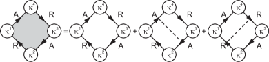
Figure 2: General Hikami box (HB): shaded area represents the correction to the ’empty’ box $V_{a}$ by $V_{b},V_{c}$ containing a single impurity line (dashed). The vertices are denoted by $\kappa^{i}\in\{\sigma^{\mu},v_{1},v_{2}\}$, and R/A stands for the averaged $G_{E_{F},b}^{R/A}$.

As a result, we can unify the calculation of the $2\times 4\times 4$ HBs in Fig. 1. They can be expressed by a linear relation in terms of the general HB in Fig. 2, defined by the ’empty’ box $\mathrm{Tr}\left\{G^{A}\kappa^{1}G^{R}\kappa^{2}G^{A}\kappa^{3}G^{R}\kappa^{4}\right\}$ and the associated HBs with a single impurity line. Here, $\kappa^{i}\in\{\sigma^{\mu},v_{1},v_{2}\}$ denotes vertices in Figs. 1, 2, and in Eq. (Mesoscopic fluctuations in the spin-electric susceptibility due to Rashba spin-orbit interaction), and $G^{R/A}_{E_{F},b}(\mathbf{p})$ is the impurity averaged Green function which depends on B-field and SOI Duckheim and Loss (2006).

Next, we evaluate the Diffuson $D$ and Cooperon $C$ in Eq. (Mesoscopic fluctuations in the spin-electric susceptibility due to Rashba spin-orbit interaction), given by $D_{q}=(1/2m\tau)(1-X_{+})^{-1}$ and $C_{q}=(1/2m\tau)k(1-X_{-})^{-1}k$, where $k^{\mu l}=\mathrm{tr}\{\sigma^{2}\sigma^{\mu}\sigma^{l}\}/2$. Expanding $X^{\mu\nu}_{\pm}=\mathrm{Tr}\{\sigma^{\mu}G^{R}_{E_{F},b}(\mathbf{p})\sigma^{\nu}G^{A}_{E_{F},\pm b}(\mathbf{p}-\mathbf{q})\}/2m\tau$ in $\bar{q}=ql\ll 1$, $\beta=2b\tau\ll 1$, and $x$, we find

$$X_{\epsilon}=\left(\begin{array}[]{llll}\frac{1}{\lambda}-\frac{\bar{q}^{2}}{2}-\beta^{2}\delta_{\epsilon,-1}&-i\beta\delta_{\epsilon,-1}&0&0\\ -i\beta\delta_{\epsilon,-1}&\frac{1}{\lambda}-\frac{\bar{q}^{2}}{2}-\frac{x^{2}}{2}-\beta^{2}\delta_{\epsilon,-1}&0&ix\bar{q}\cos\varphi\\ 0&0&\frac{1}{\lambda}-\frac{\bar{q}^{2}}{2}-\frac{x^{2}}{2}-\beta^{2}\delta_{\epsilon,+1}&-\beta\delta_{\epsilon,+1}+ix\bar{q}\sin\varphi\\ 0&-ix\bar{q}\cos\varphi&\beta\delta_{\epsilon,+1}-ix\bar{q}\sin\varphi&\frac{1}{\lambda}-\frac{\bar{q}^{2}}{2}-x^{2}-\beta^{2}\delta_{\epsilon,+1}\end{array}\right)\,,$$ (8)

where $\varphi$ is the polar angle of the momentum $\bar{\mathbf{q}}$ and $\lambda=1-i\Delta\tau$. We will find below that the main contribution to $\overline{\delta\chi^{2}}$ comes from the $1/\bar{q}^{2}$ terms in $D^{00}$ and $C^{33}$. To account for orbital dephasing we introduce a corresponding dephasing time $\tau_{\phi}$ in $D$ and $C$ by the standard replacement (see e.g. Eq.(3.15) in Bergmann (1984)) $\Delta\rightarrow\Delta+i/\tau_{\phi}$.

Although generalized to include spin vertices, the method presented so far involves the calculation of similar diagrams as for the conductance fluctuations Altshuler (1985); Akkermans and Montambaux (2007). An important difference, however, is the inclusion of the vertex corrections for spin and spin-dependent velocity which we discuss now. The vertex correction is an infinite sum of diagrams which consists of non-crossing impurity lines connecting the retarded and advanced Green functions in either $\chi^{ij}$ or $\chi^{km}$, resp. For the velocity vertex this leads to $v_{j}\rightarrow p_{j}/m$, i.e. the spin part of the velocity is cancelled in the dc limit Chalaev and Loss (2005). For the spin vertex this leads to the replacement $\sigma^{i}\rightarrow\Sigma^{i\mu}\sigma^{\mu}$ where $\Sigma$ is diagonal given by $\Sigma=(1-X_{+})^{-1}$ at $\bar{q}=0$, with the relevant entries $\Sigma^{11}=\Sigma^{22}=2/x^{2}$ and $\Sigma^{33}=1/x^{2}$. These expressions are valid in the regime $l/L\ll x$ and will be used here. For general $x,L$, the finite size form of the vertex correction has to be taken into account, giving e.g. $\Sigma^{22}=(2/x^{2})(1-\tanh{(xL/2l)}/(xL/2l))$, which then renders Eq. (11) given below finite for $x\to 0$.

In the regime $\mathrm{max}\{(l/L)^{2},\tau/\tau_{\phi}\}\ll x^{2}$, we find for the in-plane ($i=1,2$) and out-of-plane ($i=3$) components of the variance

$$\overline{(\delta\chi^{ij})^{2}}=\left(\frac{e\delta\bar{q}^{2}}{8\pi^{3}v_{F}}\right)^{2}\sum_{n_{x}=1,n_{y}=0}^{\infty}s^{ij}(\bar{q}_{n_{x}},\bar{q}_{n_{y}})\,,$$ (9)

where $v_{F}=p_{F}/m$ is the Fermi velocity, $\delta\bar{q}=\pi l/L$, and the sum over the $\bar{q}_{n}\equiv\delta\bar{q}n$ satisfies the mixed boundary conditions for the Diffuson Akkermans and Montambaux (2007) in a finite sample of square size $L$ with two opposite sides attached to the leads. Here, $s^{ij}$ in Eq. (9) are rational functions in $\bar{q}_{n_{x}},\bar{q}_{n_{y}}$ depending parametrically on $x$, $\mathbf{b}$, $\Delta$, and the orbital dephasing rate $\phi=\tau/\tau_{\phi}=2l^{2}/L_{\phi}^{2}$.

Evaluating $s^{ij}$ for $l/L,l/L_{\phi}\ll x$ first for $b=\Delta=0$, and choosing the E-field along x (i.e. $j=1$) we find

$$s^{i1}=\frac{a_{i}\left(4x\Sigma^{ii}\right)^{2}}{(\bar{q}^{2}+2\phi)^{2}}\,,$$ (10)

where $a_{1}=a_{2}=1$ and $a_{3}=2$. From Eqs. (9), (10) we then obtain $\overline{(\delta\chi^{i1})^{2}}=(ex\Sigma^{ii}/2\pi^{3}v_{F})^{2}c_{2}a_{i}$, where $c_{2}=\sum_{n_{x},n_{y}}\delta\bar{q}^{4}/[(n_{x}^{2}+n_{y}^{2})\delta\bar{q}^{2}+2\phi]^{2}$. To assess the magnitude of this result we compare it to the average of the in-plane susceptibility $\overline{\chi^{21}}=ex/2\pi v_{F}$ Edelstein (1990). For the out-of-plane component of the spin fluctuations this yields

$$\frac{\overline{(\delta\chi^{31})^{2}}}{(\overline{\chi^{21}})^{2}}=\frac{2c_{2}}{\pi^{4}x^{4}}=\frac{c_{2}}{2\pi^{4}}\frac{\tau_{DP}^{2}}{\tau^{2}}\,,$$ (11)

and similarly for the in-plane components. Thus, we see that the relative fluctuations grow with increasing $\tau_{DP}$, where $\tau_{DP}=2\tau/x^{2}$ is the D’yakonov-Perel spin relaxation time D’yakonov and Perel (1972).

Remarkably, for negligible dephasing, i.e. $\phi\ll 1$, one obtains $c_{2}\approx 1.51$, and the spin fluctuations $\overline{(\delta\chi^{ij})^{2}}$ become independent of the sample size. Typical numbers for a GaAs 2DEG (that are consistent with the regime of validity for $L_{\phi}=10l$) yield $x=0.1\dots 1$ and thus result in large relative fluctuations, $\sqrt{\overline{(\delta\chi^{ij})^{2}}}/\overline{\chi^{21}}\approx 20\dots 0.2$. In other words, there exist specific impurity configurations and realistic system parameters that give rise to a large out-of-plane spin polarization in response to a static in-plane electric field.

Figure 3: Example of a propagation path along which an initially y-polarized spin (small arrow) rotates exclusively into the positive out-of-plane z-direction (denoted by circled dots). The spin directions are denoted by small arrows at the left of each segment and result from precession about the instantaneous Rashba spin-orbit field.

To gain physical insight into this result, we consider an electron with spin initially pointing along the $y$-axis, see Fig. 3. While the electron propagates coherently through the sample, the spin precesses about the intrinsic Rashba SOI field which is in-plane and perpendicular to the propagation direction. As a result of orbital phase coherence the electron propagates along a path that is preferred by constructive interference in the given disorder configuration. Fig. 3 shows an example of such a path and the spin directions associated with the propagation through each segment. Along this entire path the spin can only point up ($+z$-direction), but never down. Now, if initially the electrons were unpolarized, the net out-of-plane polarization in this case would be cancelled by spins that are initially pointing along the negative $y$-direction. However, due to the (in-plane) MEE, which itself is subject to strong fluctuations, e.g. due to conductance fluctuations, there is a finite in-plane polarization to begin with. The cancellation is therefore incomplete. These considerations make plausible that disorder configurations exist that give rise to strong out-of-plane spin polarizations.

We next consider the effect of an in-plane magnetic field. For $b=0$ we see that the terms a) and d) in Eq. (Mesoscopic fluctuations in the spin-electric susceptibility due to Rashba spin-orbit interaction) contribute equally to the variance. However, for $b\neq 0$ the $1/\bar{q}^{2}$-divergence is cut off in the Cooperon and we can approximate Eq. (9) by making use of

$$s^{ij}_{b}\approx s^{ij}_{b=0}\frac{1}{2}\left[1+1\Big{/}\left(1+\frac{32(b\tau)^{2}}{(\bar{q}^{2}+2\phi)x^{2}}\right)\right]\,,$$ (12)

where the first term in Eq. (12) results from the Diffuson contribution (the term containing $V_{La},V_{Ra}$ in Eq. (Mesoscopic fluctuations in the spin-electric susceptibility due to Rashba spin-orbit interaction)) which is not affected by (moderate) magnetic fields.

Figure 4: The relative variance of the out-of-plane spin susceptibility $\overline{(\delta\chi^{31})^{2}}/\overline{\delta\chi^{21}}^{2}$ is shown as a function of the in-plane magnetic field $2b\tau$ for $x=0.1$, $L_{\phi}=100l$, and sample sizes $L=100\pi l$ (solid line) and $L=200\pi l$ (dashed line), resp. The low field approximation, Eq. (12), (curved dotted line) and half of the $b=0$-value (straight dotted line) are shown for $L=\pi l100$. Inset: Variance as a function of $\Delta$ for $x=0.1$, $L_{\phi}=100l$, and $L=100\pi l$ (solid line) and $L=200\pi l$ (dashed line). The suppression of $\overline{\delta\chi^{31}}$ with increasing $b$ and $\Delta$ is described by Eqs. (12) and (13).

Unlike the magnetic field, a difference in energies $\Delta$ (e.g. induced by gate voltages) leads to a suppression of all terms contributing to $\overline{\delta\chi^{2}}$. This is described by

$$s^{ij}_{\Delta}\approx s^{ij}_{\Delta=0}\Big{/}\left(1+\frac{4(\Delta\tau)^{2}}{(\bar{q}^{2}+2\phi)^{2}}\right)\,,$$ (13)

which gives rise to a correlation scale for susceptibilities at different gate voltages. Indeed, according to Eq. (13), we can regard $\chi(E_{F})$ and $\chi(E_{F}+\Delta)$ as uncorrelated for $\Delta\geq\mathrm{max}\{\phi/\tau,(\pi l/L)^{2}/\tau\}$.

In conclusion, we find strong mesoscopic fluctuations of the spin-electric susceptibility in a disordered 2DEG due to Rashba SOI, giving rise to a large out-of-plane polarization. The predicted values and dependences on the SOI strength, B-field, dephasing rate, and Fermi energy are well within experimental reach. Such spin-dependent coherence effects, besides being of fundamental interest, might prove useful in spintronics applications aiming at the electrical control of spin polarization.

We thank O. Chalaev, O. Tsyplyatyev, and B. Altshuler for discussions. We acknowledge financial support from the Swiss NF and the NCCR Nanoscience Basel.

References

- Awschalom et al. (2002) D. D. Awschalom, D. Loss, and N. Samarth, eds., Semiconductor Spintronics and Quantum Computation (Springer, Berlin, 2002).
- Awschalom and Flatté (2007) D. D. Awschalom and M. E. Flatté, Nature Physics 3, 153 (2007).
- Levitov et al. (1985) L. S. Levitov, Y. V. Nazarov, and G. M. Eliashberg, Zh. Eksp. Teor. Fiz. 88, 229 (1985).
- Edelstein (1990) V. M. Edelstein, Solid State Comm. 73, 233 (1990).
- Kato et al. (2004a) Y. K. Kato, R. C. Myers, A. C. Gossard, and D. D. Awschalom, Phys. Rev. Lett. 93, 176601 (2004a).
- Kato et al. (2004b) Y. K. Kato, R. C. Myers, A. C. Gossard, and D. D. Awschalom, Nature 427, 50 (2004b).
- Kato et al. (2005) Y. K. Kato, R. C. Myers, A. C. Gossard, and D. D. Awschalom, Appl. Phys. Lett. 87, 022503 (2005).
- Silov et al. (2004) A. Y. Silov et al., Appl. Phys. Lett. 85, 5929 (2004).
- Stich et al. (2007) D. Stich et al., Phys. Rev. Lett. 98, 176401 (2007).
- Meier et al. (2007) L. Meier et al., Nature Phys. 3, 650 (2007).
- Bychkov and Rashba (1984) Y. A. Bychkov and E. I. Rashba, J. Phys. C 17, 6039 (1984).
- Akkermans and Montambaux (2007) E. Akkermans and G. Montambaux, Mesoscopic physics of electrons and photons (Cambridge Univ. Press, 2007).
- Altshuler (1985) B. L. Altshuler, Sov. JETP Lett. 41, 648 (1985).
- Altshuler et al. (1991) B. L. Altshuler, P. A. Lee, and R. A. Webb, eds., Mesoscopic Phenomena in Solids (Elsevier, 1991).
- Lee et al. (1987) P. A. Lee, A. D. Stone, and H. Fukuyama, Phys. Rev. B 35, 1039 (1987).
- Zumbühl et al. (2005) D. M. Zumbühl et al., Phys. Rev. B 72, 081305(R) (2005).
- Miller et al. (2003) J. B. Miller et al., Phys. Rev. Lett. 90, 076807 (2003).
- Aleiner and Fal’ko (2001) I. L. Aleiner and V. I. Fal’ko, Phys. Rev. Lett. 87, 256801 (2001).
- Duckheim and Loss (2006) M. Duckheim and D. Loss, Nature Physics 2, 195 (2006); Phys. Rev. B 75, 201305(R) (2007).
- Chalaev and Loss (2005) O. Chalaev and D. Loss, Phys. Rev. B 71, 245318 (2005); ibid. 115352, 77 (2008).
- Zyuzin (1990) A. Y. Zyuzin, Europhys. Lett. 12, 529 (1990).
- Engel et al. (2006) H.-A. Engel, E. I. Rashba, and B. I. Halperin (2006), cond-mat/0603306.
- Walls and Heller (2007) J. Walls and E. Heller, Nano Letters 7, 3377 (2007).
- Bardarson et al. (2007) J. H. Bardarson, I. Adagideli, and P. Jacquod, Phys. Rev. Lett. 98, 196601 (2007).
- Krich and Halperin (2008) J. J. Krich and B. I. Halperin (2008), arXiv.org:0801.2592.
- Oestreich et al. (2005) M. Oestreich, M. Römer, R. J. Haug, and D. Hägele, Phys. Rev. Lett. 95, 216603 (2005).
- Bergmann (1984) G. Bergmann, Phys. Rep. 107, 1 (1984).
- D’yakonov and Perel (1972) M. I. D’yakonov and V. I. Perel, Sov. Phys. Solid State 13, 3023 (1972).